1. Introduction
After the 11 September 2001 terrorist attacks on the World Trade Center and the Pentagon in the United States, interest in counter-terrorism methods with limited resources has rapidly increased. However, allocating scarce defensive resources to optimize an objective function is one of the classic problems in Operations Research [
1], being an important and difficult task [
2]. For the defense agencies in many countries, weapon system of systems (WSOS) development planning is a critical process used to develop countermeasures (CMs) to confront the threats posed by other hostile countries [
3]. The planning solution focuses on how to allocate resources to different weapons to effectively eliminate the threat from hostile countries.
In prior studies on weapons development planning, a decision maker (DM) seeks to maximize a single objective function, such as capability, profit, and effectiveness. For example, Gu et al. [
4] established a WSOS planning model by maximizing the expected effectiveness as the optimization target. Håkenstad [
5] compared the long-term defense planning systems of seven Nordic countries and found that most countries aimed to improve their own profit. Zhang et al. [
6] proposed an optimization model to minimize the capability gaps to find the best development scheme by comparing different combinations of weapons, based on the given capability requirements. Throughout the literature research, however, did not mention the change of the opponent. In contrast, this paper considered minimizing the threat caused by the enemy as the objective function. Herein, we addressed an arms race between two parties,
R and
B. Each party considers the potential threat from the other party.
R develops one or more weapons to gain operational advantages over
B, whereas
B attempts to develop one or more CMs that would neutralize, or at least mitigate, the threat from
R [
7].
Resource allocation in adversarial settings, also called the research of arms races using mathematical models, has been studied since the 1930s. However, most of these studies focused only on the strategic aspect but not the operational aspect. In 1935, Richardson [
8] first proposed a simple coupled differential equation model to solve the effects of an arms race between rival states, thus successfully predicting World War II. Later, Hunter [
9] analyzed a three-nation arms race by solving linear difference equations based on Richardson’s study. Similar to most previous research, Hunter’s model focused only on the strategic aspect and did not consider the relationship between research and development (R&D) investments and time, nor the cooperation relationships among different weapons. Afterwards, Etcheson [
3] established and solved equations to optimize the function of each side rather than the constrained nonlinear optimization model. Recently, Paulson et al. [
10] proposed a model for determining optimal resource allocation by combining game theory with a simple multi-attribute utility model. The defender first allocated her resources amongst all combinations of countermeasures and targets, and then the attacker striked with his best response to this allocation. Golany [
11] investigated efficient computation schemes for allocating two defensive resources to multiple sites to protect against possible attacks by an adversary. The availability of the two resources was constrained and the effectiveness of each may vary over the site. Mazicioglu [
12] modelled the attacker’s behavior using multi-attribute prospect theory to account for the attacker’s multiple objectives and deviations from rationality. These articles mainly modelled adversary’s behavior from macroscopic and strategic view, and considered neither the time required to develop new countermeasures, nor the relationship between expenditures and development gap. In addition, budgets were not modelled explicitly.
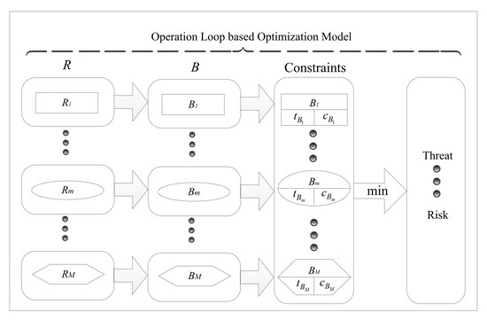
WSOS is a variety of weapons that can be functionally related to each other in accordance with a certain structure with a higher level of integration with certain strategic guidance, operational command, and security conditions [
13]. Moreover, with the development of technology, the operational effectiveness of an army depends on the interactions between multiple weapons instead of independent weapons [
14]. However, to the best of our knowledge, the relationships among different weapons have rarely been modelled in the literature. For example, the most authoritative article in Operations Research [
15] focused only on a single family of countermeasures (e.g., interception systems or bomb neutralization systems) that evolves and improves over time. With the development of informationization, the performance of defense depends on the interaction of multiple systems rather than the individual attributes of the armaments. As a consequence, the defender tends to use several families of CMs instead of a single type, so the performance of the defense cannot be determined only by the effectiveness of any single CM employed. Instead, the cooperation between CMs should be considered. Furthermore, as new CMs are introduced, even in the decision-making stage, the defender may also have to consider the interaction between the current CMs and future possible CMs to optimize the defense system. If the relationships among weapons are ignored in the development planning process, the problem will be simplified to a simple selective problem of a single weapon, neglecting the holistic structural characteristics [
16]. Thus, we used and improved an operation loop-based network model focusing on the cooperation relationships among the weapons [
17], in which weapons are represented as nodes, whereas relationships among the weapons are modelled as edges. In this model, weapons entities contain sensor, decision, influencer, and target nodes. All types of nodes are treated as target nodes to the enemy. Note that one weapon may be characterized as multiple nodes, and each node is attached to a parameter, denoting the amount of the resources allocated to it. In addition, we considered the real link rules of these nodes that prior studies [
18] did not mention. For example, if more than one
S node exists in one operation loop, the nodes could only be arranged based on their index values of
Radius in descending order. Due to the limitation of the geographical locations of the different weapons and some other factors, not all nodes could transfer information or energy, and certain nodes could only be arranged in descending or ascending order. This phenomenon is common in real-life operational battles.
In summary, this problem can be modelled as a constrained nonlinear optimization problem, which is known as NP-hard. The complexity of this type of problem depends on the complex relationships among weapons. Consequently, we argue that the analytical solution to the problem is not feasible, and a heuristic-based optimization algorithm would be effective. In this article, we used Differential Evolution (DE) and Non-Dominated Sorting based Genetic Algorithm-II (NSGA-II) for our optimization tasks.
The main contributions of this paper are as follows: (1) When assessing the threat posed by the enemy, we not only considered the cooperation among different nodes based on the traditional ideology of the operation loop, but also the real link rules of these nodes. Meanwhile, the system dynamics principle was used to characterize the dynamic behavior of the nodes in the complex weapons network; (2) According to the characteristics of the weapon life cycle curve, we considered some realistic constraint conditions, such as the annual weapons budget, the total weapons budget, and the weapon planning cycle; (3) A complex multi-objective planning problem and the related solving approach were proposed, considering the development risks and probabilistic threat from the enemy. In this paper, we considered practical settings in realistic dynamic competition.
This paper was organized as follows.
Section 2 introduced the modeling method based on operation loop and the threat assessment process.
Section 3 elaborated upon the single objective optimization model with time and investment constraints. In addition, the algorithm to solve the problem was outlined.
Section 4 extended the objective functions to an actual weapons R&D process.
Section 5 demonstrated the usefulness of the models by presenting the results of a numerical experiment. Finally,
Section 6 concluded the paper and discussed possible future research.
2. Problem Formulation
Throughout history, two or more countries are often in hostilities, such as the United States and the Soviet Union during the Cold War, India and Pakistan, and so on. Therefore, WSOS development planning transforms from a capacity to a military demand, as seen as an arms race. The R&D of national military weapons occurs in a situation requiring rapidity of development. Each country will set the other country or countries as the “reference” or “opponent” and change their own R&D strategies following the change of the R&D strategies of the opponent. Herein, we considered the dynamic competition between two parties, denoted as the attacker (
R) and the defender (
B). Generally speaking,
R is a military power with advanced military technology and in a leading position in the military.
R will independently develop a set of new weapons early on to attack
B to gain an advantage at time
tR1. The weapons developed by
R are targets that
B must counter. If all information about
R is obtained by the intelligence department of
B completely and opportunely at time
tR1, then the initial damage (
d1) caused by
R, typically measured in casualties and economic damages [
15], to
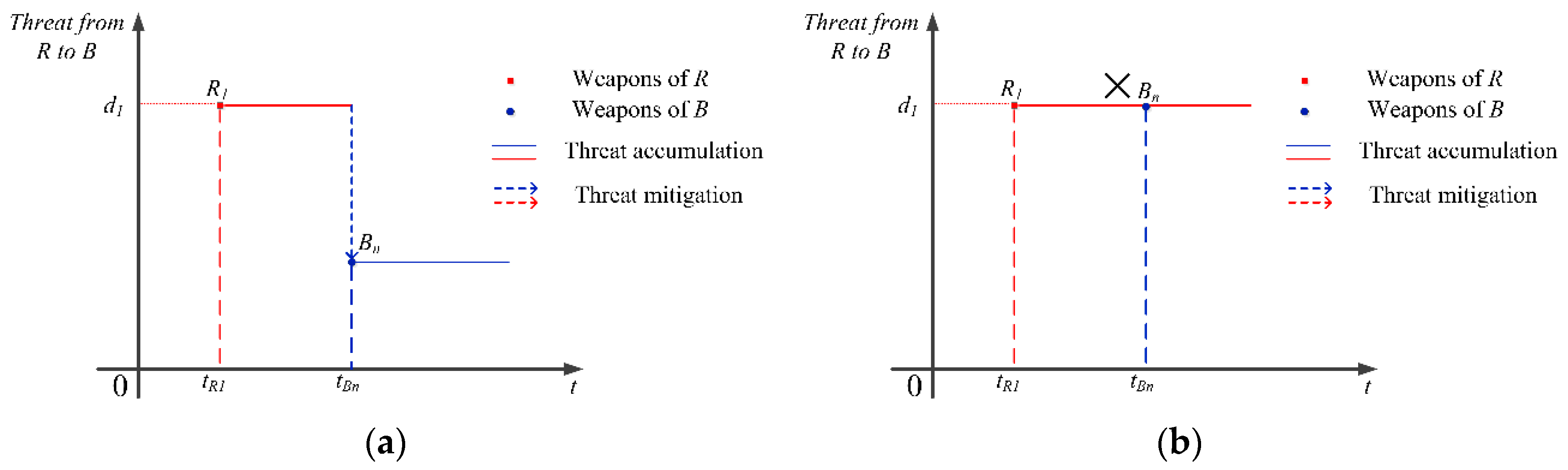
B is known. As shown in
Figure 1a, to defend the homeland from being attacked by
R,
B must develop new weapons (
Bn) as CMs to mitigate the damage. However, as shown in
Figure 1b, if
B cannot intercept information about
R’s new weapon or
B’s CMs fail, the threat will remain.
The collection of different weapons is called WSOS. Modern weapons are complex, integrated, and diverse. The connections among weapons also vary. Therefore, we not only considered interdependency among the current weapons, but also relationships among all current and future weapons. In this paper, the concept of meta-functional nodes and meta-functional edges, based on the operation loop, was used to model the cooperation relationships among weapons.
2.1. Cooperation Relationships Modeling among Weapons Based on an Operation Loop
2.1.1. Meta-Functional Node Modeling
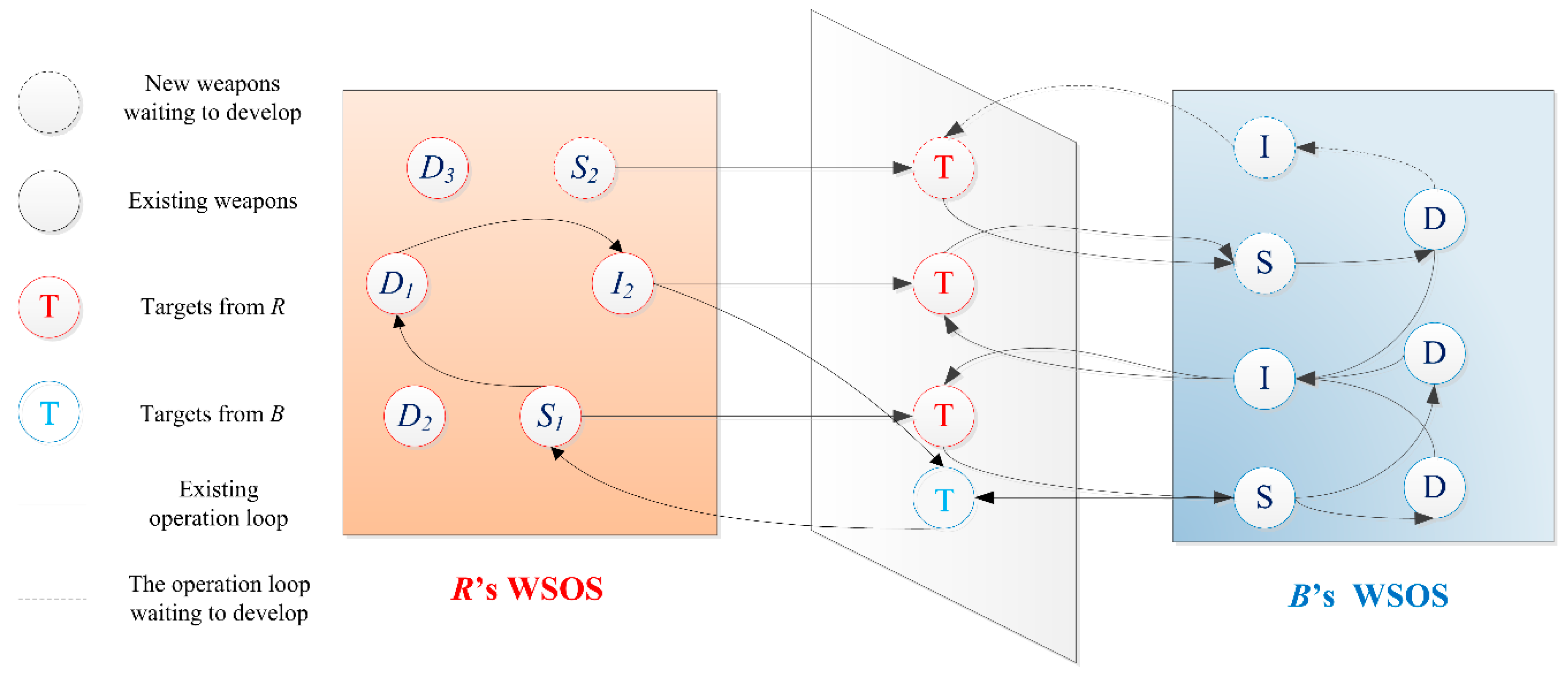
A meta-functional node can be represented as a three tuple, containing a node identity, node type, and node threat vector, as shown below:
The node identification indicates the position of the meta-functional node in combat operation process, such as red or blue. The node type refers to the classification of the meta-functional node, which can be divided into different categories from different angles. Cares [
19] divided nodes into sensor, decider, influencer, and target according to the different roles on the battlefield. In this study, meta-functional nodes were divided into four categories: scout, command-and-control, influence, and target, which are expressed as follows:
where
S,
D,
I and
T represent the meta scout functional node, meta command-and-control functional node, meta influence functional node, and meta target functional node, respectively. Node
S refers to the weapon, equipment, entity, or system that performs basic surveillance, reconnaissance, and warning in a battle, such as radar and infrared detection systems. Node
D is a system that performs basic command and control tasks during a combat operation. Node
I is a device, entity, or system that performs basic fire strikes or electromagnetic interference during a battle, such as artillery, missiles, and torpedoes. Different nodes are included in both the same and different weapons. For example, an armored observation and command vehicle can be characterized as node
S and node
D. A self-propelled antiaircraft gun can only be characterized as node
I. An illustrative example of different nodes in WSOS is provided in
Figure 2. Different parties are described with corresponding color.
R has five existing nodes (
S1,
D1,
D2,
D3 and
I2) and one new weapon (
S2) awaiting development.
S1,
S2 and
I2 can be detected by
B and become
B’s targets. The same applies to the other party.
2.1.2. Meta-Functional Edge Modeling
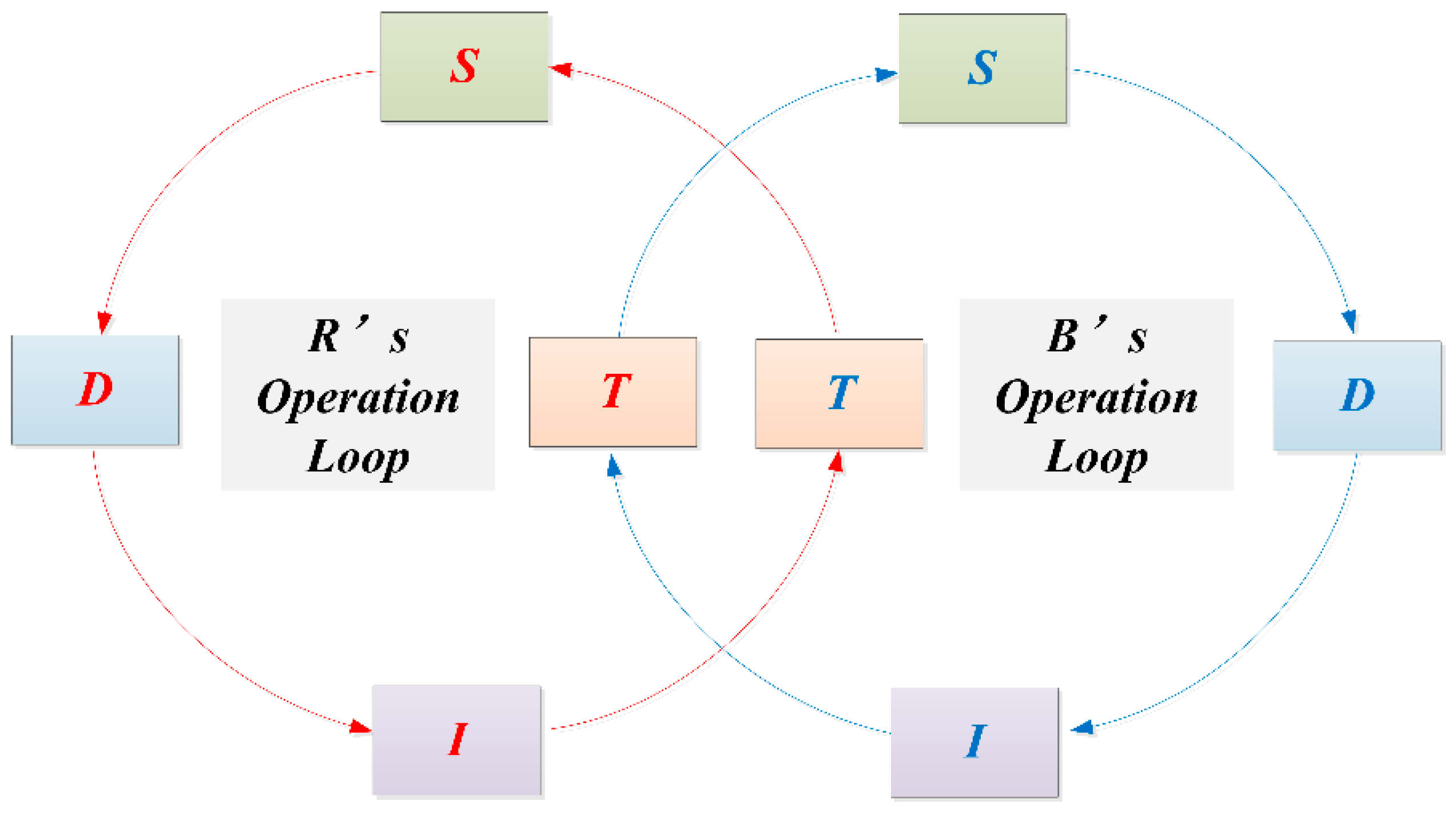
Considering the antagonism between the two sides,
B will set all of
R’s nodes as the target. Similarly,
R will set all of
B’s nodes as the target. Thus, 36 (node number × node number) different combinations of the three kinds of meta-functional nodes exist. Some types of meta-functional edges, however, do not exist in practical operation. Based on the following assumptions, we filtered the 36 edge types: (1) the node
S cannot act independently; it can only share information with other
S or
D nodes; (2) the node
D cannot attack the enemy target directly; and (3) the node
I will not interfere or attack its own weapons. After applying these filters, 20 edge relationships remained in the WSOS network under the antagonistic situation, as shown in
Table 1.
2.1.3. Operation Loop Modeling
Modern warfare theory, which is also called Observe Orient Decide Act (OODA) theory [
20], argues that a combat operation is a cyclic process. First is target discovery (
T→
S), then information is delivered to the node
D (
S→
D). Next, node
D analyzes the battlefield situation and charges node
I (
D→
I) to attack node
T (
I→
T). The close loop (
T→
S→
D→
I→
T) is called the operation loop [
21]. During the operation, both parties build their own operation loops, and treat all the opponent’s nodes as targets, as shown in
Figure 3. Although only four classes of meta-functional nodes exist in one operation loop, each type of node can contain more than one weapon. Different weapons cooperate with others through loops. The number and technical performance of loops directly impact the combat effectiveness. The greater the number of loops, the stronger the threat capability. The fewer the nodes and edges in a loop, the better the threat effect.
2.2. Threat Assessment
2.2.1. Node Threat Vector
In this study, we applied the concept of accumulative damage presented by Golany [
15], which is an objective function that measures the threat posed by the opponent. To assess the threat of the whole WSOS, we first analyzed the node threat vector. Different types of nodes have different functions, and the corresponding threat vectors vary considerably. Based on prior studies [
22,
23,
24], we improved the index system of different nodes. The threat vector of the node
S is:
where
Radius,
Accuracy,
DetectRate and
HavestRate denote the reconnaissance scope, the target recognition accuracy, the effective detection rate, and the critical intelligence acquisition rate of the node
S, respectively. The threat vector of the node
D is
where
CoverRate,
Efficiency,
Community and
Dlay represent the effective coverage rate, the information processing efficiency, the network communication efficiency, and the command decision time of the node
D, respectively. The threat vector of the node
I is
where
Radius,
Accuracy,
RPG and
Mobility indicate the operational coverage radius, the hitting accuracy, the ammunition quantity, and the maneuvering speed of the node
I, respectively.
means that the vector can be extended to different weapons.
2.2.2. Tactical and Technical Index Normalization
The different indicators have different dimensions. For example, the unit of the operational coverage radius is km, and the unit of the maneuvering speed is km/h. Therefore, different index values have to be standardized. The quantitative indexes are divided into two categories: the benefit type and the cost type. The greater is the value of the benefit index, the greater is the threat. The greater is the value of the cost index, the lesser is the threat. For example, the higher is the hitting precision of the node
S, the os higher the threat. The shorter is the decision time of the node
D, the sooner the attack can be implemented, resulting in a greater threat. The processing methods of the two quantitative indicators are as follows:
where Equation (6) is the standardized function of the dimensionless benefit index and Equation (7) is the standardized function of the dimensionless cost index.
I is the original index.
Imax and
Imin are the worldwide maximum and minimum values of the current index, respectively. As for the benefit index, if the value of
I reaches
Imax, the score of the index is 1. Otherwise, the score is 0. The same logic applies to the function symbol of the cost index.
2.2.3. Threat Assessment Based on Operation Loop
The basic goal of the WSOS is to strike the opponent targets and reduce the opponent combat capability, until that capability is completely lost. Hence, threat assessment should emphasize the influence on enemy targets. Each operation loop in the WSOS represents a method to strike the enemy target. As a result of the differences in the performance of the weapons within the operation loop, the threat to enemy targets varies. After normalization of the index value, we classified and aggregated the threat value of the various nodes. The weighted sum method was used in this paper, as it is the most commonly used index aggregation method. The method assigns weight
wj to each index, and then weights the sum to obtain the threat value
dj of one node.
An operation loop contains the node set
S, the node set
D, and the node set
I. The threat to the opponent target of the entire operation loop is
where
ds,
dd, and
di represent the threat vector aggregation value of node
S, node
D, and node
I, respectively. The total threat to the opponent is the sum of all loops.
2.2.4. Initial Threat Rate and Threat Accumulation
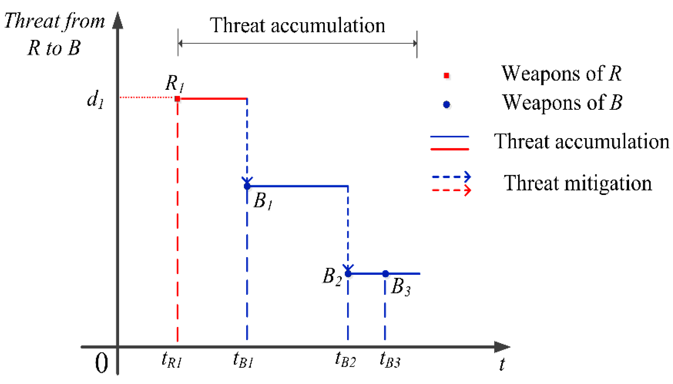
The goal of the development of new weapons is to reduce the threat from the opponent. The threat that changes over time is determined by the performance of one’s own weapons. For example,
Figure 4 shows the dynamic change in the threat from
R during the development process of
B. The horizontal axis represents time and the vertical axis represents the threat. The red squares represent the deployment of
R’s weapons and the blue dots represent the deployment of
B’s weapons. The threat from
R increases after
R’s new weapon
R1 is deployed. Then, the threat accumulates for a period of time. Once
B has developed new weapons against
R,
R’s threat level decreases. Then,
R develops new weapons to increase the threat again. That is to say, the threat changes with the deployment of new weapons, and accumulates over time.
B selects
B1,
B2, and
B3 from the optional weapons collection.
B1 and
B2 form operation loops that cover
R with other weapons, and the threat from
R decreases. Although
B develops
B3, it cannot form an operation loop that covers
R. Therefore, the threat from
R remains unchanged.
In summary, B must choose the most suitable weapons against R, and rationally plan the development. In addition, weapons must be deployed as soon as possible to neutralize the threat that accumulate with time.
2.2.5. Evaluation of Threat Reduction Effects
According to the real-life military operations, B develops new weapons to form operation loops to mitigate the threat from R. The number of operation loops represents the number of ways in which the opponent targets can be attacked. The higher the number of operation loops, the more ways are available to cover the opponent target nodes, and the better the threat reduction effect.
The WSOS network is complex dynamical network system. To research this kind of problem, the dynamical theory is usually introduced into the nodes of the complex network. In a complex network, the dynamic behavior of each node is governed by two factors: the original dynamic behavior mechanism of the node itself, and the influence of the nodes to which they are connected. Considering a complex dynamical network system that is coupled to
N nodes, the general expression is [
25]:
where
denotes the state of node
vi at time
t;
f(
xi(
t)) denotes the primitive dynamic behavior of node
vi;
c is the coupling coefficient;
g(
xj(
t)) denotes one coupling function through the coupling relationships among nodes; and
A = (
aij)
N×N is the topological structure or adjacency matrix of the complex network, and every element is positive. If
aij = 0, no connection exists between node
i and node
j. Conversely, if
aij ≠ 0, a relationship between node
i and node
j exists. Next, we combined the actual nature of the WSOS to establish a dynamic WSOS network model based on the general model.
From the analysis of the operational process outlined in
Section 2.2.4, we knew that the formation of the operation loop of
B reduced the threat from
R. As a result, the coupling coefficient
c was −1. The coupling function
g(
xj(
t)) was calculated using Equations (8) and (9). We assumed that the number of new operation loops was
m during
B’s weapons development process, and only the operation loops that covered
R’s threat nodes reduced the threat from
R. Thus, not all
m operation loops reduced the threat from
R. The value of
aij has the following two forms:
In summary, the cumulative threat (
DB) expression is:
where
denotes the threat from the entire WSOS of
R at time
t;
f(
x(
t)) denotes the initial threat caused by
R, namely, the situation where
B’s confrontation is not considered; and
denotes a measure of threat reduction.
3. Single Objective Modeling and Solving
Golany [
7] viewed an arms race as a process between two asymmetrical groups. The advantage established by one side is temporary, and the advantage disappears when the other side exceeds it. Therefore, the issue faced by
B is how to use limited resources to develop effective CMs to mitigate the threat from
R as much as possible. Thus, the cumulative threat is used as the optimization objective function. To simplify the computation, we only considered the operation loops that cover the threat nodes of
R. Consequently,
aij is removed from the expression. Then, all new
m loops work to counter
R. The initial threat from
R is set as
d1. The entire duration of the confrontation is expressed as
T. The number of
B’s operation loops that cover
R is
m, and the moment of forming of the
jth loop is
tj. Then, the cumulative threat expression is:
3.1. Constraints
In the WSOS development planning process, B must consider the following two constraints: time and money.
3.1.1. Time
The cumulative threat posed by R gradually increases over time. Supposing B chooses to develop 10 new weapons. If all investments are made at time 0, then the optimal choice is that the development of the 10 new weapons is initiated at time 0. Therefore, B can deploy new weapons to counter R more rapidly. If not all investments are made simultaneously, but in batches due to the limited investments amount for each batch, B must consider the sequence of these new weapons. Therefore, the starting time and R&D time of the weapons directly impact the threat reduction. Herein, time is considered as a constraint, including the beginning and throughout the duration of the operation.
The starting time (
stBj) of each weapon should satisfy the following relationship:
The upper limit of the R&D duration should be less than the weapon development planning; otherwise, this development planning would be meaningless. The lower limit of the R&D duration depends on the technical maturity of R&D. Therefore, the R&D duration (
tBj) should be between the shortest and longest development time length:
3.1.2. Investment
To date, the research on the weapons funding allocation problem is still prominent, focusing on limited budgets and how to allocate resources to different weapons. Therefore, R&D investments should be considered as a constraint, including the single weapon budget, the annual budget, and the total budget.
The upper and lower limits of R&D investment usually depend on defense funds. If the investment is too small, the weapon will fail to develop. Similarly, the investment has an upper limit that cannot be more than the assigned national defense funds. Therefore, the R&D investment (
cBj) of each weapon should be between the minimum and maximum investments:
The total investment for all new weapons should be lower than the total budget (
C):
Although the total investment was confirmed prior to creating the development plan, the R&D funds are often used in batches because of a long development period of many years or even decades. This article focused on a five-year planning problem. Thus, the total investment
C was divided into average usage over five years. A strict capital flow restriction was placed on the annual budget. Moreover, the unused budget for one year could not be carried over to the next year. We assumed that the funds are continuously and evenly invested in the development of one weapon. As multiple weapons were being developed in one year, the annual investment in the
Hth year should not exceed
C/5:
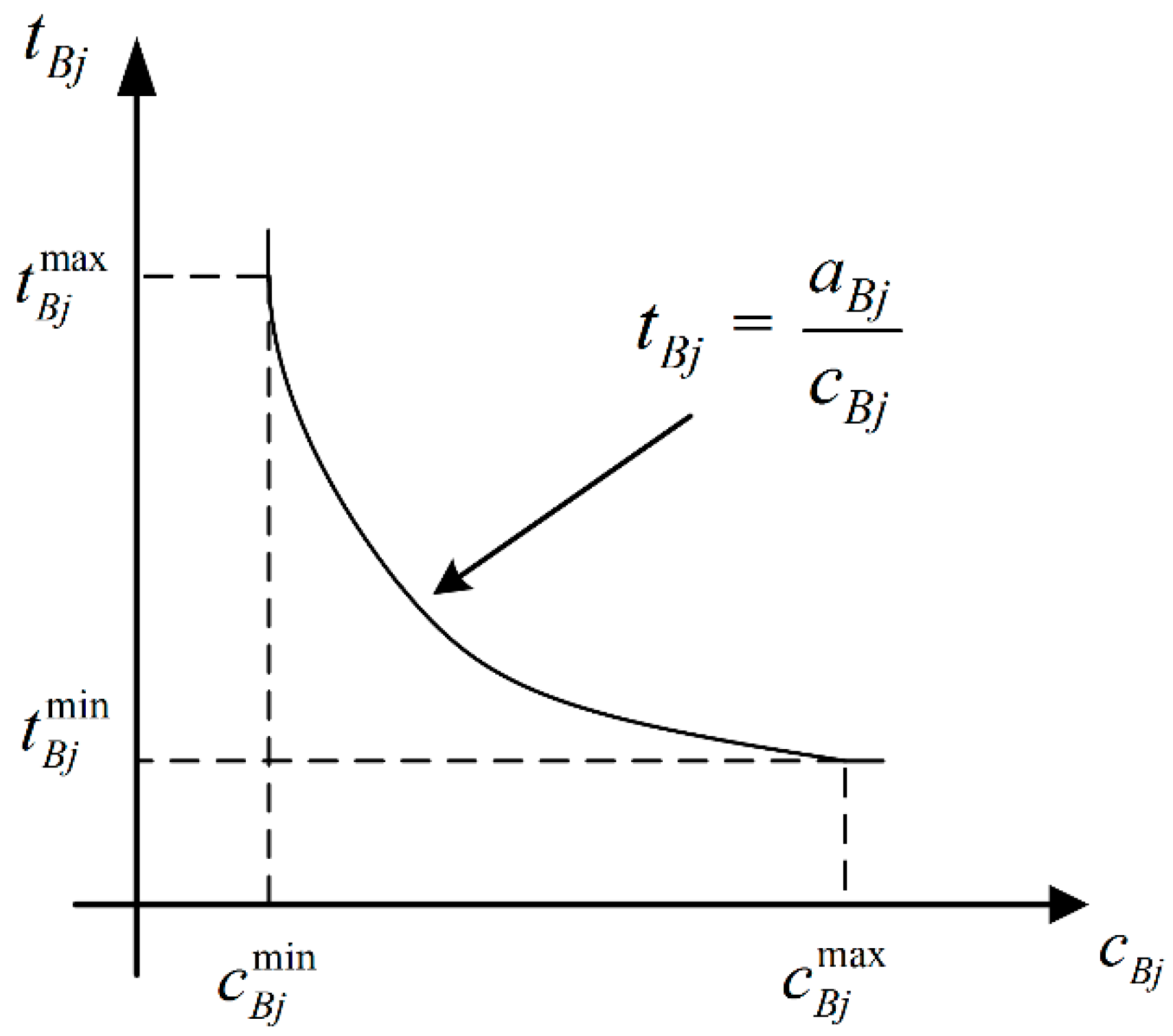
3.2. Modeling the Relationship between Time and Investment
In reality, a negative correlation exists between the R&D time and investment. To ensure the smooth development of weapons, the investment of each weapon cannot be lower than a certain threshold
cmin, otherwise it will not be successfully developed. The lowest investment amount corresponds to the longest development time
tmax. As the investment gradually increases, the development time correspondingly gradually shortens. However, as the marginal effect of investment decreases, the development time declining rate slows. In addition, due to technical restrictions, the development time cannot continually decrease. No matter the amount of the investment, the development time will not be less than the shortest time
tmin. The corresponding investment is now
cmax. Therefore, for the relationship between time and investment, the inverse scaling function model was designed as shown in
Figure 5. Herein,
aBj generally represents the technical difficulty in the development process.
The relationship above is simple. However, we argue that a realistic relationship between development time and the resource investments can only be empirically determined from experts or statistically from data. This problem is neither a major concern in this paper, nor a key component of our model.
In Golany’s model [
15],
tBj was used to determine the development time of each weapon.
tBj was determined by the level of intensity, which is a discrete variable; therefore,
tBj was also a discrete variable. As opposed to Golany’s model,
tBj =
aBj/
cBj is used to describe the development time, determined by the allocated investment, which is quite realistic in defense contracting. The continuous variable
cBj implies continuity of
tBj, resulting in a wider range of possible solutions. Hence, the problem faced by
B is to decide which weapon to develop, when to start development, and what proportion of the available resources to allocate to each weapon based on the current weapons. The objective is to minimize the cumulative damage over the time horizon, subject to budgetary constraints.
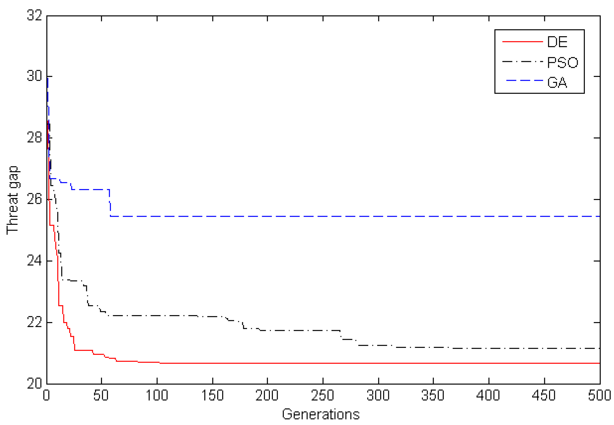
3.3. Algorithm Design
The decision variables of the problem are development time and investment amount. The unit of development time is usually years. The unit of investment is usually millions or an order of magnitude higher. For easy figures, all variables take integers. We defined the solution space as
S, and the corresponding scale as:
The scale of S increases exponentially with an increase in n. The computational complexity of this problem is at least NP-hard. Therefore, using an intelligent optimization algorithm for solving this problem is reasonable.
Differential Evolution (DE) is an evolutionary optimization methods proposed by Storn and Price [
26]. A simple mutation operation and a one-on-one competitive survival strategy reduce the complexity of a genetic operation. DE is robust and has a strong global convergence ability, suitable for solving certain optimization problems that conventional mathematical programming methods cannot solve in complex environments [
27]. Given the advantages of DE and the characteristics of this model, we designed the following solving algorithm.
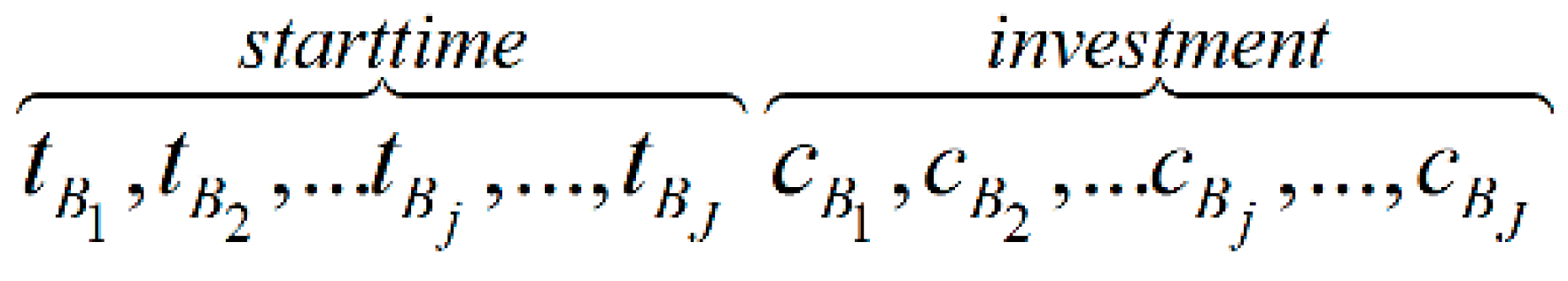
Step 1: Initialize the population. Using decimal integers to encode all variables according to the type of decision variables is appropriate for this problem. A total of
J pending weapons exist, so an individual of 2
J is generated. The encoding form of the individual is shown in
Figure 6.
The upper boundary for time in terms of the variable is five, whereas the lower boundary is one, which respectively indicates that the weapon is developed in the fifth or the first year. As for the investment, the upper boundary is cmax and the lower boundary is cmin.
Step 2: The fitness function and penalty function. Evolutionary algorithms have been widely used to solve optimization problems. However, when the optimization problem has many nonlinear, linear, inequality, and equality constraints, the solving process is more complex. Therefore, designing a constraint processing technology with better performance is essential. Michalewicz [
28] and Coellol [
29] conducted extensive investigations into the constraint handling techniques and classified the techniques into five classes: penalty functions, special representations and operators, repair algorithms, separation of constraints and objectives, and hybrid methods. Among these constraint handling approaches, we applied the penalty functions to address the constraints. We set the development investments, so that the planning each year that exceeded the annual budget is the penalty function. The fitness function is defined as the objective function. The smaller is the fitness value, the better is the individual. The penalty function
f is:
where each part in Equation (20) denotes the extent to which the corresponding limit is exceeded. Taking the first item
as an example, when the annual investment exceeds the budget, the first item is
. Herein, the part of the excess budget is computed as part of the penalty function. Conversely, if
, the corresponding penalty function is 0. That is, no violation of the constraint is triggered. As for the time,
stBj should take an integer between 1 and 5. If the starting time of a weapon does not meet this requirement, the excess is computed in the penalty function
. The same logic is applied to the other constraints.
Step 3: Initial population evaluation. The fitness value and the degree by which each individual in the population violates the constraints are calculated. When no individual violates the constraints in the population, the penalty function is 0. Then, the individual with the best fitness value is the current global optimal solution. When all individuals in the population violate the constraints, the penalty functions of all individuals are greater than 0. Then, the individual with the least penalty function value is chosen as the current global optimal solution.
Step 4: Mutation operation. Equation (21) is used to mutate the individual.
where
Xbest is the best target individual;
xr1(
G),
xr2(
G), and
xr3(
G) are random target individuals;
vi(
G + 1) is the mutant individual, and
F ∈ [0, 1] indicates the mutant scale factor, recommended as 0.5 [
30].
Step 5: Crossover operation. To increase the diversity of the population, the crossover operation is performed between the temporary individual and the parent individual. Substitute the parent individuals for temporary individuals with a probability of CR = 0.2.
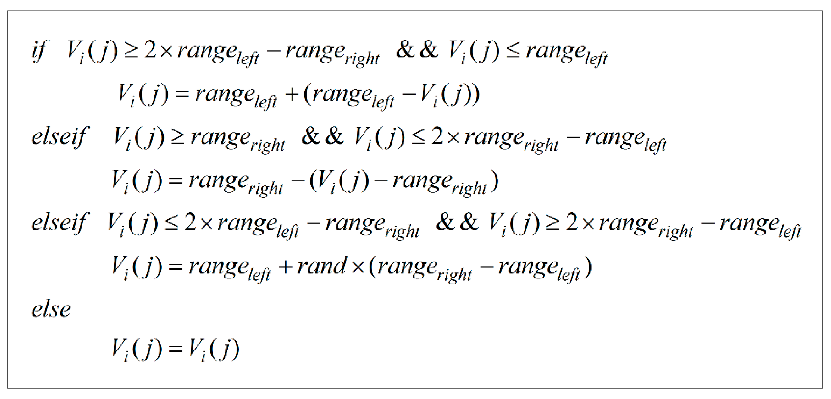
Step 6: Cross-border processing. The classical DE does not consider how to address the constraints handling. The randomness of the general cross-border processing strategy is too strong to preserve the historical optimal information accumulated through evolution. We used the symmetric mapping processing strategy as previously reported [
31]. As shown in
Figure 7,
rangeleft and
rangeright are the left and right boundaries of each variable in the individual, respectively. When the extent to which a variable violates the constraint is less than the absolute value of the variable range, the boundary point is taken as the center to map this variable equidistantly onto the range of value.
Step 7: Competitive survival operation. We used the idea of competition survival to compare the fitness and penalty function of the corresponding individual in the parent population and temporary population, and selected the preferable individual to form a new population. The specific rules are: (1) if both individuals do not violate the constraints, we judge them by comparing their fitness values; (2) if a solution satisfies the constraints, whereas the other one does not, then the solution meeting the constraints is better; and (3) if both do not meet the constraints, the solution with the lower penalty function is better.
Step 8: Evolution and iteration. We determined whether the scheduled iterations are reached. If so, then the operation is stopped; otherwise, proceed to step 3. If the desired iterations are reached, but the satisfactory solution has not been found, the population size and the iterations should be adjusted.
6. Conclusions
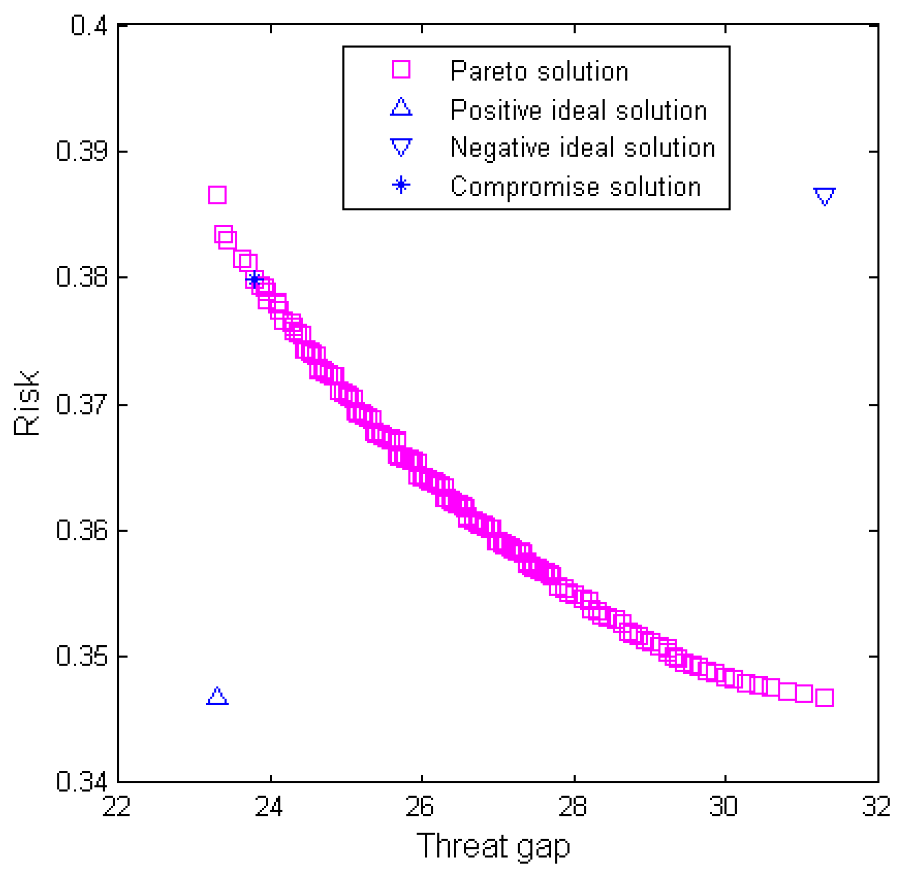
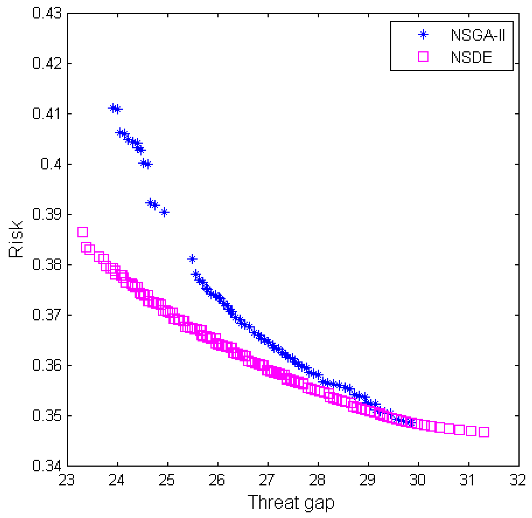
This paper proposed a new approach to solve the problem of allocating limited resources when developing military CMs versus probabilistic threat, with emphasis on representing the cooperation relationships among different weapons. The competition between hostile countries was transformed into an operation loop-based optimization model. We applied the system dynamics principle to characterize the dynamic behavior of the nodes in a complex weapons network. The intrinsic properties of a weapon were converted into certain constraints. To address the development of CMs with limited resources to counter the enemy, the threat gap was set as the single objective function. In addition, considering the uncertainties in the development process, the R&D risks of weapons were used to optimize the planning. Ultimately, certain intelligent optimization algorithms were used to obtain a numerical solution.
The numerical results showed that more investments result in a more effective design, and more time leads to lower risk. The key weapons that can effectively reduce threat and could potentially encounter technical difficulties during R&D should be developed as soon as possible. With a fixed investment amount, the results also demonstrate that the system effectiveness can be significantly improved by increasing the amount allocated to the weapon that is found in more operation loops.
Future research directions include allowing for uncertainty in players’ preferences, having a dynamic resource distribution strategy over a certain time horizon, and enabling multiple players or multi-objective in a sequential game. These challenges will contribute to the expansion of this methodology for tackling a broader range of problems.


