1. Introduction
The concept of the supercritical CO
2 Brayton cycle was first proposed in the 1960s [
1,
2], but research progressed slowly at that time for various reasons. With the global energy and environmental problems highlighted and the progress of manufacturing technology, the supercritical carbon dioxide Brayton cycle has regained attention and is expected to be used in many fields [
3], including nuclear energy, solar energy, and geothermal energy etc., as displayed in
Figure 1.
Among various working fluids, supercritical carbon dioxide attracts more attention due to its unique advantages: (1) SCO2 is one of the most common supercritical fluids with relatively low critical pressure and temperature (7.3773 MPa, 304.13 K). (2) The high density and convective heat transfer coefficient of SCO2 make it able to reduce the volume of turbomachines and heat exchangers. Compared with steam turbines, SCO2 turbines are only about 1/100 of the size, so the SCO2 Brayton cycle has an obvious advantage regarding construction costs. (3) The low viscosity and strong mobility of SCO2 can reduce the flow resistance. (4) Compression works are largely reduced due to the low compressibility factor, accounting for about 20–30% of the turbine output power, which would improve the efficiency of thermal cycle.
Compared to the helium Brayton cycle and the conventional Rankine steam cycle, the same net efficiency can be achieved by the SCO
2 cycle at a lower temperature, which means that it is less expensive than the others. Furthermore, the net efficiency of the SCO
2 cycle was shown to be significantly less sensitive to penalties from core bypass flow and cycle pressure drops than the helium Brayton cycle [
4].
However, because the working pressure is so high and the size is so small, decent efficiency of the equipment is difficult to achieve, which leads to much lower experimental cycle efficiency than is expected. Due to the large density of SCO2, the compressor’s volume flow rate is so small that the blade height is much shorter than that of an air compressor. Narrow flow channels will cause high friction losses and leakage losses. Meanwhile, as the compressor operates near the critical point, the fluid properties are very different from those under normal temperature and pressure. Therefore, it is necessary to study the design method for supercritical CO2 compressors.
Yong Wang et al. (2004) designed axial flow compressors for a 300 MWe SCO
2 power cycle with Concepts NREC-AXIAL
TM and predicted efficiency as high as that of large mass flow rates [
5], as shown in
Table 1. Yifang Gong with his co-workers (2006) designed centrifugal compressors for the same power level using Balje diagram [
6], as displayed in
Table 2. But neither of them did a 3D calculation for their design results. There are also many other universities and research institutes that have carried out relevant research on the design strategy of SCO
2 compressors [
7,
8,
9,
10,
11,
12] and some research institutes have carried out experiments [
13,
14,
15].
More recently, Rinaldi (2014) and colleagues utilized an in-house fluid dynamic solver and simulated the test compressor of Sandia National Laboratories (SNL) based on the steady state method [
16]. However, their numerical simulation was not in good agreement with SNL’s experimental results. They thought this difference was caused by the limitation of CFD and the uncertainty of the experimental data. In 2014, Monje and his colleagues applied the Aungier’s one-dimensional model to design a compressor of the 10 MW central receiver type for solar plants [
17]. Results of their 1-D model are in good agreement with the simulation of Fluent software. In their calculation, the realizable
turbulence model was employed. Kim (2014) carried out a comparison between CFD and experimental results [
18]. It was found that when the inlet parameter was far away from the critical point, CFD calculation could get fairly good results. However, when the inlet condition was approaching the critical point, their deviation became more and more obvious. Yuqi Wang et al. (2017) carried out steady and unsteady numerical simulations of a SCO
2 centrifugal compressor with ANSYS-CFX [
19], which showed that the difference between the two results is small. But, it should be pointed out that the equation of state used in their calculation is not accurate enough for SCO
2.
Figure 2 and
Figure 3 are the test components of SNL and Institute of Applied Energy (IAE), respectively. These experimental results have verified the feasibility of the one-dimensional design method of the SCO
2 compressor and pointed out that windage loss is an important cause of low cycle efficiency.
However, according to the authors’ knowledge, the influences of compressor type and working parameters on design results that were obtained by conventional design methods for air have not been studied so far. The accuracy of loss models for SCO2 compressors has been rarely researched, but its importance is obvious.
At present, centrifugal compressors are studied by many more research institutes than axial flow compressors are. To the authors’ knowledge, there is still no conclusion about which type is more appropriate for the SCO2 Brayton cycle. Thus, in this paper, the design of axial flow compressors and centrifugal compressors are both carried out and the design results will be used for comparison. In the design process, CFD will be applied to test one-dimensional design results due to the lack of reliable experimental data. Furthermore, a series of mass flow rate situations will be studied to find out the limitations of the conventional models.
2. Axial-Flow Compressor Design
The design method of an axial-flow compressor is based on the flow coefficient and work coefficient, which are defined as follows:
In the design of the mean streamline method (1−D), the main flow losses include four parts as follows; profile loss, endwall loss, secondary flow loss, and tip clearance loss. It is hard to reach supersonic conditions for SCO
2 due to its large density, so there is no need to consider shock wave loss. The relative total pressure loss coefficient is defined as follows, which can also be extended to the absolute coordinate system for stators.
3. Models for the Axial-Flow Compressor
Here, empirical constants K1 = 0.004, K2 = 1, which should have been set by the experimental results.
Secondary flow loss [
21]
where
.
4. Mass Flow Rate Estimation
In order to reduce the mass flow rate error between the one-dimensional design and the CFD result, a simple mass flow rate model was built. If the direction of inflow is axial, according to the energy equation:
Hence, the mass flow rate can be calculated (assume that
tmax = 0.1
c and the exit section is straight):
Deviation angle model [
22]
Revised De Haller stall criterion [
20]
It is worth noting that this criterion is most reliable for speeds greater than about 85% of the design speed. In addition, the design parameters are limited by other conditions at the same time, for example, inlet blade angle , no negative reaction, and flow coefficent ϕ < 0.5 is preferred. So the available range of the flow coefficient and work coefficient become quite limited.
5. 1-D Design and CFD Calculation for the Axial Compressor
In order to verify the accuracy of the model and estimate the efficiency of the axial-flow compressor, an axial-flow compressor with the following parameters, shown in
Table 3, has been constructed.
Smith chart for optimum different reaction stages, which is based upon model tests of a range of axial compressor, is helpful for engineer to make a preliminary design [
23]. But the chart may overestimate efficiency and overly pessimistically estimates stall range [
20]. According to the Smith chart, once the flow coefficient has been determined, sensible range of work coefficient lies between the following two curves [
23].
The axial flow compressor in this paper adopted free vortex flow with axial outflow and hub-shroud ratio was 0.7, hence the sensible range of flow and work coefficient as
Figure 4:
To avoid a large area of condensation, the work coefficient is slightly larger than the optimum value. Thus, the corresponding flow coefficient and work coefficient are selected as 0.33 and 0.3, respectively. In order to ensure the stable operation requirements, the calculation result shows that at least 9 stages are needed to avoid stalling. In addition, the tip clearance of the rotor is 2% of the blade height. The one-dimensional design result is displayed in
Figure 5.
As there are so many stages, only the first stage was calculated with CFD to evaluate the reliability of the axial compressor’s loss models. At the same time, because the deviation angle model is not reliable at off-design conditions, which would bring about a large amount of error in prediction, only the design condition was calculated by the mean streamline method. The preliminary geometric parameters of the compressor were computed by an internal MATLAB code coupled with the NIST database and geometric modeling was completed in Numeca Autoblade. In order to reduce the amount of calculation, a single passage grid was employed and the interface between the rotor and stator was dealt with in the mixing plane. The H-block was located upstream and downstream of the blade and the O-block was applied in the rotor and stator passage. The total number of grid cells is 629,680. The geometry and grid are displayed in
Figure 6.
In order to take the real gas properties of SCO
2 into account, look-up tables were used during the calculation. These property tables were generated by the SW equation of state, in addition, they had been encrypted with logarithmic distribution near the critical point. But, if the property tables are too dense, the time of calculation will increase sharply, and it is easier to diverge. According to Ameli’s study [
24], the range of the property table is 3–28 MPa and 270–500 K for pressure and temperature, respectively, and the resolution of the tables is 300 × 300. This range is sufficient for the three compressors in this article.
Figure 7 shows the density table employed in the CFD calculation.
To ensure the reliability of the CFD, grid independence and y+ (<200) were taken into account and turbulence model was chosen as
(Extended Wall Function) model. Compared with the
model, it is more accurate near the wall layers and is more suitable for adverse pressure gradient flows, which reduces the problem of grid-induced separation for industrial flow simulations [
25]. Another advantage of the
model is its robustness near the wall treatment. Even if y+ is above 100, the computed wall shear-stress error is less than 2% [
26]. Bourgeois (2011) compared the steady-state mixing plane predictions using four turbulence models, including
,
,
,
, for a centrifugal compressor stage and showed that
and
are more accurate, but the calculation time required by the
was five times that of other models [
27]. The results of the CFD and mean streamline method (design point) are compared in
Figure 8.
As we can see, the 1-D method can predict an axial flow compressor’s performance at the design point within the allowable error range. Thus, we can use mean streamline method to estimate the overall performance of a multistage axial flow SCO
2 compressor at the design point. The result of the prediction is shown in
Figure 9.
According to
Figure 9 as the number of stages increases, the efficiency of each stage decreases seriously. The last stage’s efficiency is 7.3% lower than the first stage. In the past, it was considered that an axial compressor is more suitable for a large flow situation than a centrifugal compressor. However, due to the large density of supercritical carbon dioxide and condensation problem, the inlet axial velocity and circumferential velocity are seriously limited, which means an axial flow compressor requires quite a few stages to achieve the target pressure ratio. Because re-compressing the compressor’s inlet condition is far from the critical point, it requires more stages than the main compressor. In fact, about 20 stages are required for a re-compressing compressor. So many stages would reduce a compressor’s efficiency and reliability and increase the facility costs. Therefore, future research should focus on centrifugal compressor design and analysis.
6. Centrifugal Compressor Design
The design method for centrifugal compressors is based on the specific speed and specific diameter which are commonly used by industry for radial turbomachinery. Since the external losses cannot be considered in the CFD calculation, only the internal loss models are added into 1-D code. Furthermore, as the empirical parameters in the Two-Zone model may not be suitable for supercritical carbon dioxide compressors, a Single-Zone model is adopted. For centrifugal compressors, losses are calculated by the stagnation enthalpy. Impeller losses were evaluated with the Aungier’s loss model. Wang et al. used this model to design a very low coefficient centrifugal compressor [
28]. As for the diffuser, a more common model was used.
For a centrifugal compressor:
7. Models for Centrifugal Compressor
Blade velocity difference
Impeller skin friction [
29]
Length of blade mean camber line:
Due to the path curvature of a centrifugal compressor, the modified equation of White (1932) [
30] was used for the friction coefficient. But, it needs to be noted that the friction coefficient is also influenced by adverse pressure gradient, which is usually ignored by 1-D calculation.
Hub-to-shroud loading loss [
29]
Mean streamline curvature
represents the length of mean streamline.
Abrupt expansion loss [
29]
Mixing loss [
29]
where
.
Velocity of clearance gap leakage flow
Vaneless diffuser loss [
29]
In the vaneless diffuser, the friction coefficient is distinctly different of that inside a pipe. Thus, the experimental equation of Japikse (1982) was adopted [
31].
Diffuser outlet loss
where
is the loss coefficient.
8. Stall Criteria
- (1)
- (2)
- (3)
- (4)
- (5)
As long as any one of the above criteria is satisfied, the condition is judged to be stalled.
9. A Centrifugal Compressor for a 10 MWe System
In order to evaluate the accuracy of traditional centrifugal compressor models, the design of a 10 MWe supercritical carbon dioxide Brayton cycle compressor was carried out, and the design parameters are shown in
Table 4.
ns −
ds diagram was widely used in radial turbomachinery design, as Smith chart in axial turbomachines. As ilustrated in
Figure 10, impeller efficiency is relatively high when the specific speed is 0.55–0.7 [
37]. Thus, the specific speed was chosen to be 0.6 in the design stage. Then, we can obtain the preliminary design result of the SCO
2 centrifugal compressor.
One-dimensional design was completed with an internal MATLAB code. The 3-D geometry of the centrifugal compressor is displayed in
Figure 11 and the tip clearance of the impeller is 2% of the local blade height. In the design, the impeller outlet flow angle is 71° in order to decrease mixing loss. The flow coefficient and work coefficient are 0.042 and 0.6, respectively.
Like the axial compressor, the flow field was calculated by Numeca Fine/Turbo. The difference is in the topology of the grid. H blocks are used not only for upstream and downstream, but also for the upside and downside of the blades, but not for the blade skin. The total number of grid cells is 863,167, seen in
Figure 12. To ensure calculation convergence, the CFL(Courant Friedrichs Lewy) number cannot exceed 0.3. The
(Extended Wall Function) turbulence model was selected for the existence of separation in centrifugal compressors.
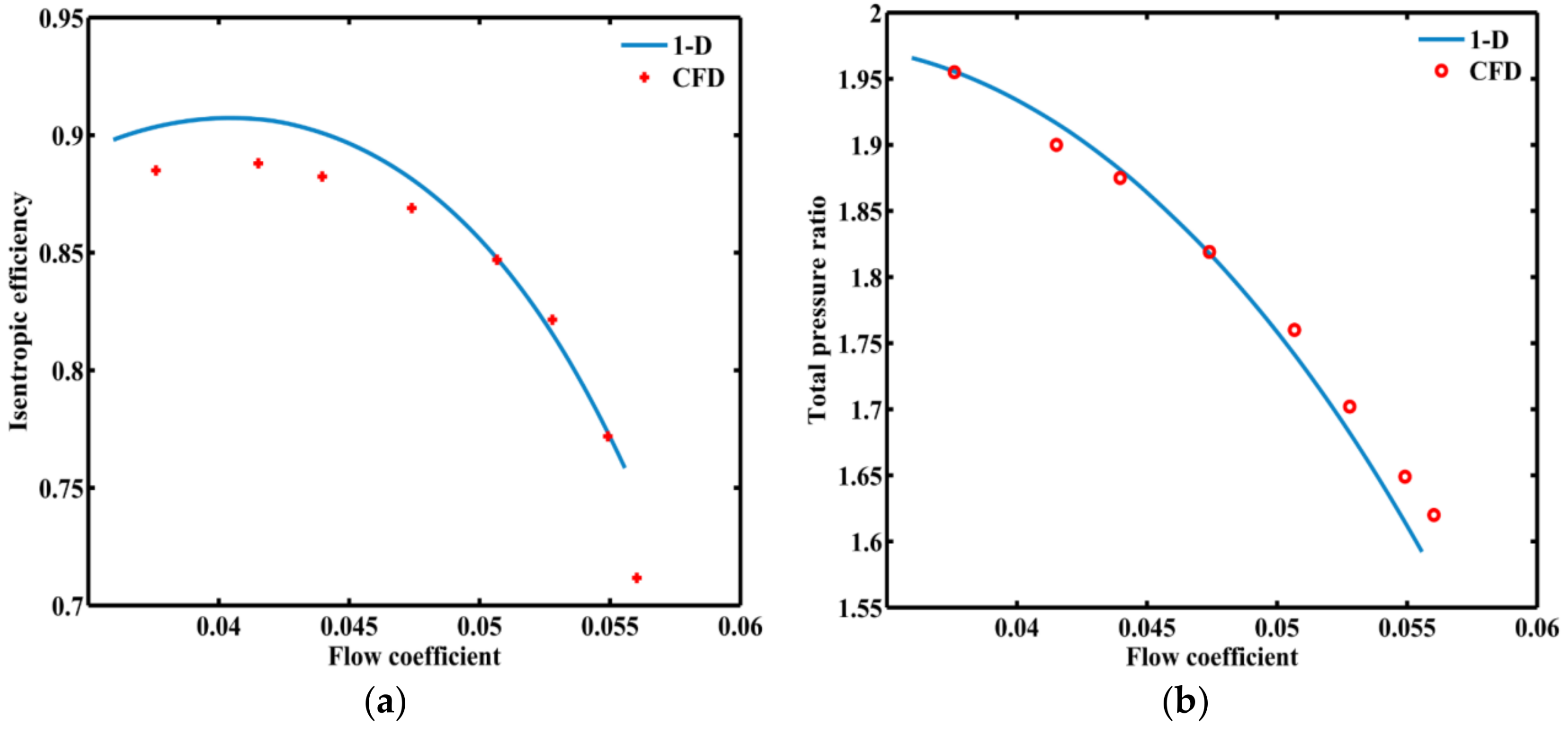
As this article is concerned with the performance of the compressor rather than flow field detail, steady state simulation was preferred. The efficiency and pressure ratio of the compressor are displayed in
Figure 13.
It is obvious that the loss models have predicted the performance of the SCO
2 compressor for a 10 MWe SCO
2 Brayton cycle reasonably well. However, the one-dimensional program predicts a greater efficiency value. In order to evaluate the influence of the SCO
2 compressor’s flow rate and loading onto deviations, the authors have designed another centrifugal compressor, which is a main compressor for a 1 MWe SCO
2 Brayton cycle, and the design parameters are given in
Table 5.
10. Centrifugal Compressor for a 1 MWe System
The design process is the same as before, but due to manufacturing technology limitations, the tip clearance of the impeller is 0.26 mm, which accounts for 13% of blade height at the impeller outlet. Because of the high pressure ratio, the impeller outlet flow angle is 63° to delay vaneless diffuser stalling and to guarantee a sufficient stall margin. Meanwhile, to avoid condensation and ensue structure strength safety, the inlet axial velocity is limited. Finally, the flow coefficient and work coefficient are 0.04 and 0.65, respectively.
The design result is shown in
Figure 14. The setting of CFD is similar to that of 10 MWe, as mentioned above. When grid independence and y+ (<200) values are guaranteed, the results of the mean streamline method and CFD are compared in
Figure 15. As for a relatively low flow and high loading compressor, the prediction of the working range of the compressor is also satisfactory. Hence, it is believed that the original stall models were also applicable to supercritical CO
2 compressors. But, the mean streamline method is overly optimistic about the performance of the compressor, especially near choke conditions. In other words, the traditional loss models should be modified.
11. Simplified Model
To find out the deviation source, additional research has been conducted. Values of an impeller (1 MWe) with no clearance was calculated by Numeca and the result was compared with Aungier’s prediction model in
Figure 16 to estimate the clearance loss.
As can be seen in
Figure 16, the result of efficiency estimation is more accurate if there is no clearance. Thus, it can be concluded that the ratio of clearance loss should have been underestimated in the original model. In fact, the original clearance loss model does not take the interaction effect of clearance flow and main flow into account. When a small flow of fluid is injected into the mainstream flow, as illustrated in
Figure 17, the total entropy creation can be obtained by the continuity and momentum balance [
38].
The leakage vortex trajectory and its radius in a centrifugal compressor is not thoroughly understood. For convenience, we can utilize the following mean velocity to estimate the mainstream mixing velocity. Considering the viscous effect, the mixing velocity should be less than the average value due to momentum loss in the boundary layer or boundary layer separation.
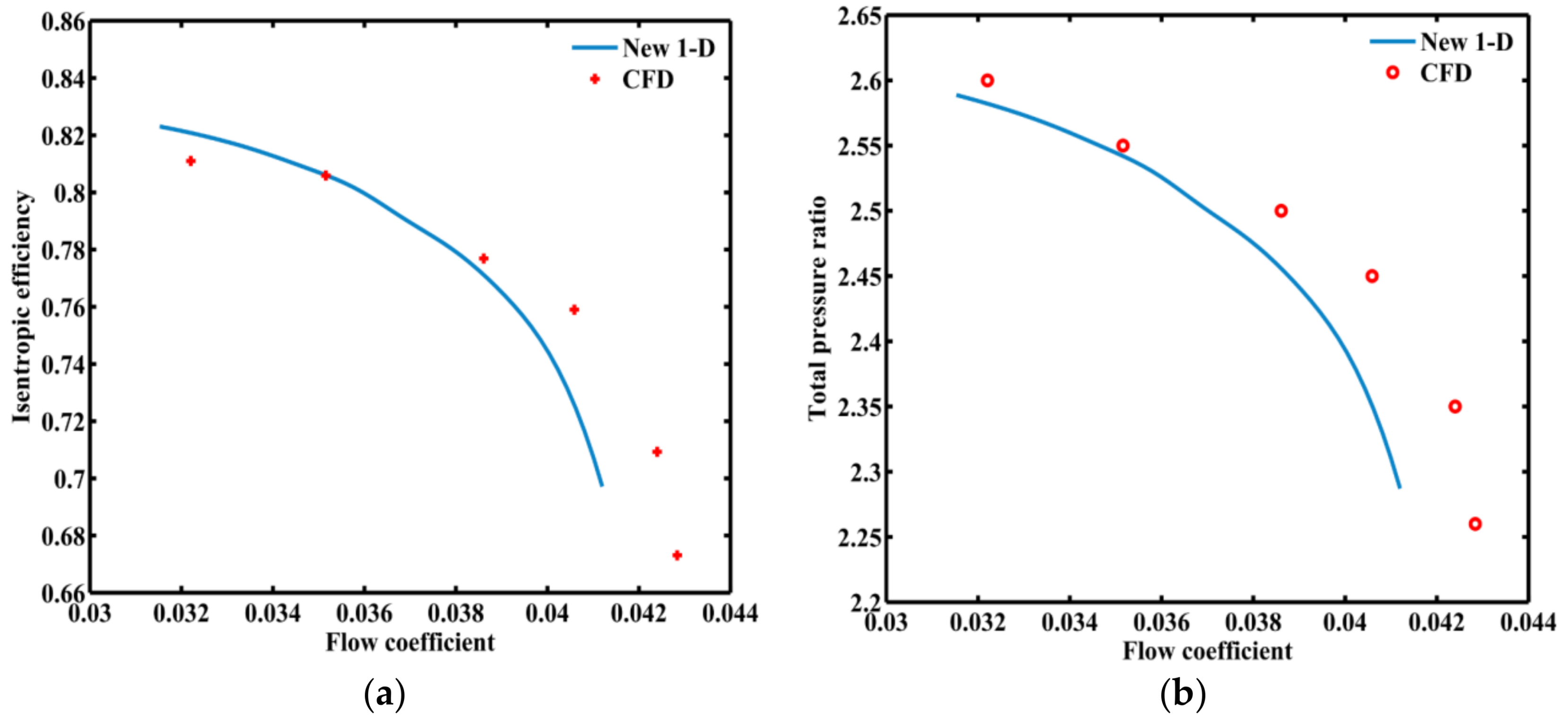
With the new clearance loss model, the performance of the impeller and stages can be predicted more precisely. In
Figure 18 and
Figure 19, the new predictions of 10 MWe and 1 MWe cycle compressors are displayed, respectively.
With the revised clearance loss model, the errors between the new 1-D model and the CFD method decrease at the design point. But, the accuracy of efficiency prediction is still not very satisfactory for off-design conditions, which is a common problem for most 1-D models. The deviation between the new one-dimensional model and CFD may be caused by two reasons. On one hand, the 1-D model itself has limitations. A centrifugal compressor is a very complex piecec of turbomachinery and the 1-D model does not match well with three-dimensional calculations under any circumstances. On the other hand, the results of the CFD may not be reliable. From the CFD calculation and experimental results of existing air compressors, there are still about 2–3% absolute errors in efficiency prediction.
12. Conclusions
Compared to axial compressors, centrifugal compressors have advantages due to their simpler structure and relatively high efficiency in SCO2 fields.
Smith charts and Balje diagrams can be also applied to SCO2 compressor design. But, actual (CFD) efficiency is lower than the prediction from the dimensionless graph. This deviation will become more serious for smaller flow rates and larger pressure ratio cases. In the authors’ view, the prediction error may be attributed to the differences in geometry. Owing to manufacturing technology and structure strength limitations, the tip clearance and blade thickness are unable to be changed proportionately.
The accuracy of the original loss models was found to be inadequate, particularly for low flow and high pressure ratio situations. Fortunately, the stall models for centrifugal compressors were found to agree with steady CFD calculations in our two cases. But, the authors also found that CFD calculation of SCO2 is much more time-consuming than air, even if a steady method with a single passage is utilized, due to the property characteristics. Therefore, the conventional unsteady calculation method for predicting the stall boundary may not be practical.
A revised method was proposed which can improve the accuracy of the prediction at the design point. In our paper, the efficiency deviation between new 1-D model and CFD is less than 3% at the design conditions. Such an error is within the allowable error range of engineering. But, to further increase the generality of model, more simulations and designs will be done in the future.


