Fault Diagnosis of Rotating Machinery Based on the Multiscale Local Projection Method and Diagonal Slice Spectrum

Abstract

The vibration signals of bearings and gears measured from rotating machinery usually have nonlinear, nonstationary characteristics. The local projection algorithm cannot only reduce the noise of the nonlinear system, but can also preserve the nonlinear deterministic structure of the signal. The influence of centroid selection on the performance of noise reduction methods is analyzed, and the multiscale local projection method of centroid was proposed in this paper. This method considers both the geometrical shape and statistical error of the signal in high dimensional phase space, which can effectively eliminate the noise and preserve the complete geometric structure of the attractors. The diagonal slice spectrum can identify the frequency components of quadratic phase coupling and enlarge the coupled frequency component in the nonlinear signal. Therefore, the proposed method based on the above two algorithms can achieve more accurate results of fault diagnosis of gears and rolling bearings. The simulated signal is used to verify its effectiveness in a numerical simulation. Then, the proposed method is conducted for fault diagnosis of gears and rolling bearings in application researches. The fault characteristics of faulty bearings and gears can be extracted successfully in the researches. The experimental results indicate the effectiveness of the novel proposed method.

1. Introduction

Rolling bearings and gears have been widely used in varieties of rotating machineries. The phenomenon of the whole equipment downtime due to the failure of key components such as rolling bearings and gears is obvious. It is thus of great significance to study the fault diagnosis technology of them [1,2,3,4]. At present, the fault diagnosis of rotating machinery is mainly aimed at their vibration signals [5,6,7]. While they fail, the mechanical system will be accompanied by strong non-linear vibrations, and vibration signals are usually affected by the measurement error and ambient noise. Under the combined action of various factors, the dynamic behavior of gears and rolling bearings may present chaos and bifurcation. The measured vibration signal is essentially a one-dimensional nonlinear chaotic time series. The chaotic signals have a similar broad spectrum with the noisy signals in the frequency domain. For nonlinear time series, a part of the useful signal will be mistaken for the noise being filtered out if traditional linear methods are still adopted for noise reduction. This may result in distortion and deformation of the signal [8,9]. Some methods of nonlinear signal processing such as time-frequency analysis [10], wavelet transform [11,12], and multi-resolution singular value decomposition [13] have improved traditional methods, which are more dependent on the characteristic frequency components of the fault signal. If the fault characteristic frequency is weak or submerged by other signal components, it is difficult to extract effective information. At present, the problem of noise suppression is still more of a concern in the field of mechanical equipment fault diagnosis, and the main purpose is to maximize the fault characteristics.

With the development of nonlinear science, the method of noise reduction based on phase space reconstruction has gradually become one important tool to study nonlinear systems. A one-dimensional time series is reconstructed into high-dimensional phase space through delay embedding. The dynamic characteristics hidden behind original one-dimensional nonlinear time series are revealed by studying the motion characteristics and distribution of the attractor in the high-dimensional phase space [14,15,16,17,18]. The attractor of the useful signal in phase space is usually confined to a limited area, and the noise signal is randomly distributed in the phase space, thus the noise components in the one-dimensional nonlinear time series can be filtered out according to different distribution rules of the useful signal and the noise in the phase space. The noise reduction methods based on singular spectrum analysis [19,20] and the local projection algorithm [21,22,23] belong to this kind of algorithm, and the local projection algorithm has been widely used in the fields of speech signal processing [21] and biomedicine [23], etc.

The main idea of the local projection algorithm was originally proposed by Sauer et al. [15] in the early 1990s. After analyzing the advantages and disadvantages of various algorithms, Grassberger and Hegger [24,25] proposed an improved algorithm. In 2004, Kantz and Schreiber [16] arranged the local projection algorithm, and successfully applied it to many fields, such as speech processing and biomedical signal analysis. In 2014, Chelidze [26] proposed smooth orthogonal decomposition, a method which projects strands according to the relative position of neighboring strands, and by simultaneously exploiting temporal and spatial correlations. During smooth orthogonal decomposition, the time series is reconstructed to high dimensional phase space, and noise can be reduced during the process of projection to tangent subspace. In 2015, to deal with the centroid selection of local neighborhoods in the local projective noise reduction algorithm, Moore [27] used higher order polynomials to estimate the neighborhood centroids more accurately, and proposed an improved high-order and multiscale local projection algorithm, which was successfully applied to medical signal processing.

For decades, first-order statistics [28] (e.g., mean, variance) and second-order statistics [29] (e.g., autocorrelation functions, power spectra) have been widely used in the analysis of mechanical vibration signals, but these methods are only theoretically applicable to the analysis of linear and Gaussian signals, which requires higher orders to reflect the signal characteristics. Compared with the first and second-order statistics, the higher-order statistics have the advantages of suppressing Gaussian noise, recognizing a non-minimum phase system, and checking signal nonlinearity [30]. However, the most obvious drawback of the higher-order statistics analysis is that it requires a large amount of computation, and the amount of computation increases with the increase of order, which makes it difficult to realize the real-time calculation of a large amount of data. Thus, there is a cumulative method of slicing, in which the most used feature is the third-order cumulant diagonal slice. Such a method can not only significantly reduce the computational complexity, but also preserve the phase information and the system’s non-linear information [31].

When the gear and rolling bearing generate faults, the vibration signals are usually accompanied by large numbers of modulation phenomenon, namely the two frequency components that interact with each other [32,33]. This phenomenon produces the sum of two frequencies and the difference between the two frequencies, and the fault signal then contains significant secondary phase coupling characteristics. When the multiscale local projection algorithm is used separately, it is not easy to extract the modulation frequency component in the fault signal, while the diagonal slice spectrum can identify the frequency components of quadratic phase coupling and enlarge the coupled frequency component in the nonlinear signal. Therefore, according to the characteristics of gear and rolling bearing fault signals in mechanical equipment, a method of mechanical fault feature extraction based on the multiscale local projective algorithm and diagonal slice spectrum is proposed. Firstly, the multiscale local projective algorithm can filter out noise while maximally preserving characteristics related to the fault. Secondly, the diagonal slice spectrum can identify the frequency components of quadratic phase coupling and enlarge the coupled frequency component in the nonlinear signal. Thus, the combination of the two algorithms can achieve the fault feature extraction of gears and rolling bearings more accurately.

This paper is organized as follows. The basic principle and characteristics of the proposed feature extraction method of a mechanical fault based on the multiscale local projection algorithm and diagonal slice spectrum are introduced in the Section 2. Section 3 introduces the numerical experiments of multiscale local projection, and simulation researches of diagonal slice spectrum, which can both prove the effectiveness of the algorithm. Section 4 presents the processing of Case Western Reserve University Bearing Data [34] and applications to Drivetrain Diagnostics Simulator to verify the validity of the proposed approach described in this paper. The conclusions of the studies and necessary discussions are given in Section 5.

2. Methodology

2.1. Standard Local Projection Algorithm

Consider a series of N scalar measurements s(1), s(2), …, s(N)$\in$R from a chaotic system. By choosing the appropriate embedding dimension m and the delay time τ, it can be reconstructed into the m-dimension phase space, and each phase point in the reconstructed phase space can be expressed as:

$$X_n=(s_n,s_{n-\tau },\cdots ,s_{n-(m-1)\tau }).$$

(1)

According to the embedding theorem [24], when the fractional dimension of the system attractor is m, it needs to meet the conditions m ≥ 2d + 1. The reconstructed phase space and the original dynamic system are differential homeomorphisms, namely they have the same dynamic characteristics. In the m-dimensional phase space, the attractor that reflects the dynamics of the system is usually confined to a low-dimensional subspace m₀ (d < m₀ < m). In the case of the absence of noise interference, there is zero subspace (m − m₀) in the phase space. When noise is present, the noise is randomly distributed in the phase space, so the component in the null subspace (m − m₀) is generated by the noise. In the neighborhoods of each phase point, the eigenvalue decomposition of the covariance matrix composed of neighborhood points is performed. The subspace formed by eigenvectors corresponding to m₀ largest eigenvalues is considered as the signal subspace, and the subspace formed by the eigenvectors corresponding to the other (m − m₀) smaller eigenvalues is the noise subspace. The main content of the local projection noise reduction is to identify the noise subspace, and then subtract the projection of the phase point on the subspace, and the basic steps of the algorithm are as follows:

(1)

Choosing the appropriate parameters m and τ to reconstruct the noisy time series into the m-dimensional phase space.

(2)

Determine the neighborhood U_n of each phase point. There are two methods to determine the neighborhood: the fixed neighborhood number and the fixed neighborhood radius. In this paper, the former is used.

(3)

Calculate the centroid of each neighborhood point.

(4)

The covariance matrix C of each phase point is calculated, and the eigenvalue decomposition is performed, and the eigenvalues corresponding to (m − m₀) smaller eigenvalues a_q (q = 1, 2, …, m − m₀) are obtained.

(5)

Subtract the projection of the phase point on the noise subspace:

$$X_n^{\prime }=X_n-R^{-1}{\displaystyle \sum _{q=1}^{m-m_0}{\mathit{a}}_q·}[{\mathit{a}}_q·R(X_n-{\overline{X}}_n)],$$

(2)

where R is a diagonal weight matrix and is used to suppress the distortion of the elements at the beginning and end of the phase, in addition to keeping the elements stable in the middle. In this paper, R₁₁ = R_mm = 103, and R_ii = 1. ${\overline{X}}_n$ is the centroid of the neighborhood, and $X_n^{\prime }$ is the signal after noise reduction.

(6)

Return to step (2) until all data have been processed.

2.2. Multiscale Local Projection Algorithm

According to the steps of the local projection noise reduction algorithm (3), Cawley et al. [14] used the mean value of the neighborhood point as the neighborhood centroid as follows:

$${\overline{X}}_n=\frac{1}{{\mu }_n}{\displaystyle \sum _{k\in {\mu }_n}{X}_k}.$$

(3)

As shown in Figure 1, it is considered that points gather around a curve, and the local linear approximations (straight lines) are not tangents but secants. All the centroids (circles) of different neighborhoods are shifted inward with respect to the curvature, which has a great effect on the performance of noise reduction. To further suppress the noise, Sauer et al. [15] estimated the neighborhood centroid using the second order polynomial.

$${{\overline{X}}^{\prime }}_n=2{\overline{X}}_n-\frac{1}{{\mu }_n}{\displaystyle \sum _{k\in {\mu }_n}{\overline{X}}_k}.$$

(4)

As shown in Figure 2, a tangent approximation is obtained by shifting the centroid outward with respect to the curvature. The filled circle denotes the average of the centroid of adjacent neighborhoods, where the square is the corrected centroid ${\overline{X}}_n^{\prime }$. In this article, we call it the standard local projection algorithm.

Moore et al. [27] considered both the geometrical shape and statistical error of the signal in the high dimensional phase space, and proposed a multiscale selection method of the centroid, which cannot only effectively eliminate the noise, but can also better preserve the complete geometric structure of the attractors. It was confirmed that the method had a good effect on medical signals. The basic principles are as follows:

For real numbers δ > 0, the continuous moving average operator can be described as I_δ by:

$$(I_{\delta }f)(x)=\frac{1}{2\delta }{\displaystyle {\int }_{x-\delta }^{x+\delta }f(t})dt.$$

(5)

Sauer et al. [15] considered a linear combination of the centroid of the first and second order, to achieve a more accurate estimate of m-dimensional of the original signal. In analogy, it requires the equation below to hold for all monomials f_n(x) = 1 (n = 0) and f_n(x) = xⁿ (x ≠ 0) with 0 ≤ n ≤ n_max, and with n_max as large as possible.

$$f_n(0)=a_1(I_{\delta }{f}_n)(0)+a_2(I_{\delta }{}^2{f}_n)(0).$$

(6)

For odd n, both the sides of (6) are zero. Letting n = 0 and n = 2 in (6) yields a system of two linear equations with the unique solution: a₁ = 2, a₂ = −1, and then identifies the m-dimensional analogue of the operator I_δ with the centroid of points within a ball of radius δ in Euclidean m-space, resulting in the second-order local projection algorithm.

As for Equation (6), the geometric structure of the attractor is taken into consideration, so the scale factor β is introduced. It is eligible to represent f_n(0) by using a linear combination of iterated moving averages of f_n evaluated at zero for integers n, such that 0 ≤ n ≤ 5 without using moving averages of an order greater than two. It requires the following equation:

$$f_n(0)=a_2(I_{\delta }{}^2{f}_n)(0)+b_1(I_{\beta \delta }{f}_n)(0),$$

(7)

which is suitable for the situation with integers n such that 0 ≤ n ≤ 5 (β ≥ 0). It gives two solutions: a₂ = 0, b₁ = 1, β = 0, and a₂ = 4, b₁ = −3, $\beta =\sqrt{8/3}$. Then, the corresponding coefficient of the standard local projection algorithm is: a₂ = 0, b₁ = 1, β = 1.

Then, the aspects of statistical error are analyzed. For non-negative integer d, define the discrete moving average operator J_d by the following equation:

$$(J_{d}f)(j)=\frac{1}{2d+1}{\displaystyle \sum _{i=-d}^{d}f(j+i)}.$$

(8)

Let e(−2), e(−1), e(0), e(1), e(2), …$\in$ R be independent random variables with mean zero and unit variance. The e(i) can be regarded as an error, and it needs to choose values of a₂, b₁, β, which are attenuated by the operator a₂J_d² + b₁J_βd. For β ≤ 2:

$$(a_2{J}_d{}^2+b_1{J}_{\beta d})e(0)={\displaystyle \sum _{l=-\beta d}^{\beta d}(a_2\frac{2d+1-\left|l\right|}{{(2d+1)}^2}+\frac{b_1}{2\beta d+1})}e(l)+{\displaystyle \sum _{r=\beta d+1}^{2d}{a}_2\frac{2d+1-r}{{(2d+1)}^2}(}e(r)+e(-r)).$$

(9)

The result holds for β, d such that βd $\in$ Z. A limit d→∞ obviates this complication. To preserve the geometry of the underlying attractor, it needs (7) to hold for 0 ≤ n ≤ 3, resulting in a₂ = A(β) = β²/(−2 + β²), b₁ = B(β) = 1 − β²/(−2 + β²). Consider the expectation of the square of filtered error at j = 0, S_a2,b1,β,d = (((a₂J_d² + b₁J_βd)e)(0))², with these geometric constraints on a₂, b₁, β.

The desirable case of dense embedding corresponds to a large window d, while in the limit, d→∞, S_a2,b1,β,d→0. Thus, normalize the expectation S_a2,b1,β,d by that which refers to prototypical local projection proposed by Cawley [14]. This gives:

$$T_{a_2,b_1,\beta }=\underset{d\to \infty }{\lim }\frac{S_{a_2,b_1,\beta ,d}}{S_{1,0,\beta ,d}},$$

(10)

which is called the normalized expected error, and using (9) and the independence of the variables e(i), it is straightforward to compute that $T_{a_2,b_1,\beta }=2a_2{}^2/3-0.5a_2{b}_1\left(-4+\beta \right)+b_1{}^2/\beta$. Since the parameters a₂ and b₁ can be calculated directly according to β, which established the relationship between the scale factor β, and the error T(β). When β varies between [0,5], the corresponding error values are shown in Figure 3 and Figure 4. The Figure 4 is the local enlargement of Figure 4, where the error curve has a local minimum at β = β* ≈ 0.96215 (marked red in Figure 4), and further calculates a₂ = a₂* = A(β*) ≈ −0.86174, b₁ = b₁* = B(β*) ≈ 1.86174. These values are suggestively close to the coefficients (a₂ = 0, b₁ = 1, β = 1) of the standard local projection algorithm, but are more accurate. The parameter values corresponding to the local minimum point are taken as the new filter coefficients, thus a new multiscale local projection filter is established, which could effectively attenuate error while more precisely preserving geometry.

2.3. The Basic Principle of Diagonal Slice Spectrum

The most common technique in the high order spectrum is the bispectrum, which can identify the frequency components of secondary phase coupling in the nonlinear signal, but its calculation method has the disadvantage of large computation and poor precision in the process of estimating. The diagonal slice spectrum is a simplification of the bispectrum, which overcomes shortcomings of bispectrums, and improves computational efficiency and precision, while preserving the advantages of bispectrums. Therefore, it has important significance in feature extraction of the nonlinear signal.

For the stationary random process x(t) with zero mean, the third-order cumulant is defined as [35]:

$$C_{3x}({\tau }_1,{\tau }_2)=E[x(t)x(t+{\tau }_1)x(t+{\tau }_2)],$$

(11)

where E[…] represents the desired operation, and τ₁ and τ₂ represent the time delay constants. Let τ₁ = τ₂ = τ, then the third-order cumulant diagonal slice of signal x(t) can be obtained.

$$C_{3x}(\tau )=C_{3x}(\tau ,\tau )=E[x(t)x(t+\tau )x(t+\tau )].$$

(12)

It can be observed that the third-order cumulus diagonal slice is essentially a straight line passing through τ₁ = τ₂ = τ in a two-dimensional plane (τ₁, τ₂), which realizes the simplification of complex data, and transforms the two-dimensional data into one-dimensional data [36].

The discrete Fourier transform of the third-order cumulant diagonal slice is called the diagonal slice spectrum.

$$S_x(\omega )={\int }_{-\infty }^{+\infty }{C}_{3x}(\tau )e^{-jw\tau }d\tau .$$

(13)

The properties of S_x(w) can be summarized as follows:

(1)

If x(t) is a Gaussian signal, then its third-order cumulant diagonal slice spectrum S_x(w) = 0. This indicates that the diagonal slice spectrum can suppress Gaussian noise.

(2)

If the probability density function of x(t) obeys the symmetric distribution, its third-order cumulant diagonal slice spectrum S_x(w) = 0. This indicates that the diagonal slice spectrum can suppress the noise of symmetrical distribution.

(3)

If the harmonic signal has three components, the frequency and phase are respectively f_k and φ_k (k = 1, 2, 3). Assuming f₁ > f₂ > f₃, if both f₁ = f₂ + f₃ and φ₁ = φ₂ + φ₃ are satisfied, it can be concluded that the three harmonic components meet the secondary phase coupling relationship, and then S_x(w) = 0. Conversely, if these two conditions cannot meet simultaneously, then S_x(w) ≠ 0. This shows that the diagonal slice spectrum can identify the frequency components of quadratic phase coupling and enlarge the coupled frequency component in the nonlinear signal.

2.4. Feature Extraction Method of Mechanical Fault Based on Multiscale Local Projection Algorithm and Diagonal Slice Spectrum

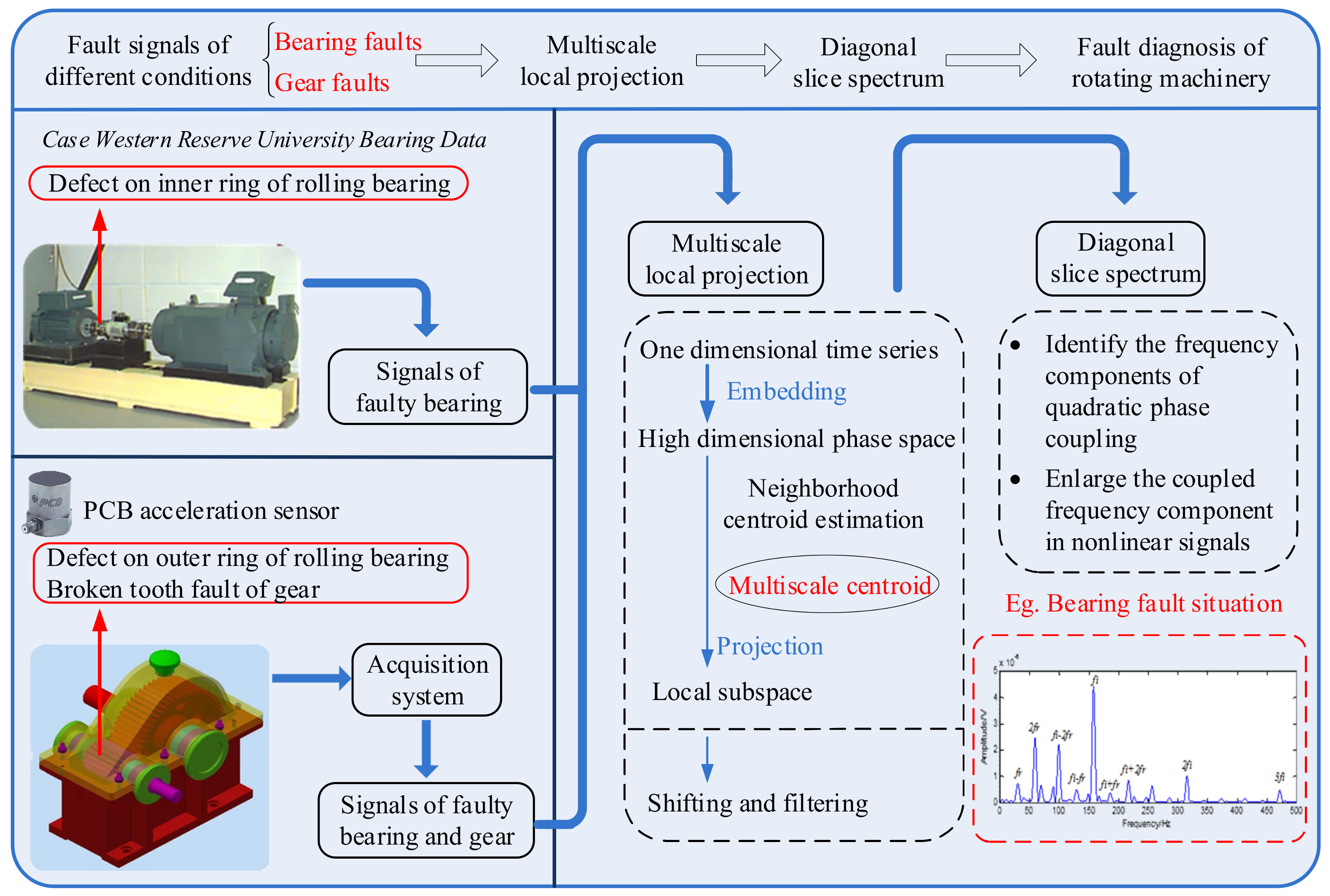
Rolling bearings and gears work long hours in complex and harsh environments, and are susceptible to various strong noises. The fault signals often have nonstationary, nonlinear, and non-Gaussian properties, and there are a lot of secondary phase coupling phenomena. When the multiscale local projection algorithm is used separately, it is not easy to extract the modulation frequency component in the fault signal. The diagonal slice spectrum can identify the frequency components of quadratic phase coupling, and enlarge the coupled frequency component in the nonlinear signal. Therefore, according to the characteristics of gear and bearing fault signals, this paper proposes a novel method of mechanical fault feature extraction based on the multiscale local projection algorithm and diagonal slice spectrum. Firstly, multiscale local projective algorithm can filter out noise while maximally preserving characteristics related to different kinds of faults. Secondly, the diagonal slice spectrum can identify the frequency components of quadratic phase coupling and enlarge the coupled frequency component in nonlinear signals. Therefore, the proposed method based on the above two algorithms can achieve more accurate results when it comes to fault feature extraction of gears and rolling bearings. The basic idea of the proposed method is illustrated in Figure 5.

3. Numerical Simulation

3.1. Numerical Simulation of Chaotic Signals

To illustrate the noise reduction effect of the multiscale local projection algorithm, the Lorenz signal is used for simulation analysis. The equation is as follows:

$$\left(\begin{array}{l}\dot{x}\\ \dot{y}\\ \dot{z}\end{array}\right)=\left(\begin{array}{l}\sigma (y-x)\\ -y+rx-xz\\ -bz+xy\end{array}\right),$$

(14)

where σ = 10, r = 28, b = 8/3, and the Lorenz system exhibits chaotic characteristics. The x component of the Lorenz system is used for simulation analysis, where sampling points N = 3000, sampling frequency f_s = 3000 Hz, and the integral step is 0.05. A certain level of Gauss white noise is added to x, and signal noise ratio (SNR) is 6 dB. Then, the multiscale local projection algorithm is used to reduce the noise. Figure 6 is the time domain diagram of the original signal, Figure 7 is the time domain diagram after adding noise, and Figure 8 is the time domain diagram after noise reduction by multiscale local projection. In Figure 9, the multiscale local projection algorithm is compared with the standard local projection algorithm. It can be concluded that multiscale local projection algorithm has a better denoising effect than the standard local projection algorithm.

To explain the advantages of multiscale local projection algorithm more intuitively, phase diagrams are adopted to show its effectiveness. Figure 10a is a phase diagram of the original signal, Figure 10b is a phase diagram after adding noise, Figure 10c is a phase diagram after noise reduction by the standard local projection algorithm, and Figure 10d is a phase diagram after noise reduction by multiscale local projection. It can be concluded that multiscale local projection can preserve the geometry of the attractor maximally in the case of filtering noise, and has a better denoising effect than standard local projection.

In addition, to illustrate the denoising effect of the multiscale local projection algorithm, the following two evaluation indicators are used.

(1)

Mean Squared Error (MSE)

$$MSE=\frac{1}{N}{\displaystyle \sum _{i=0}^{N-1}{[\tilde{x}(i)-x(i)]}^2}$$

(15)

(2)

Cross Correlation (CC)

$$CC=\frac{\langle x,\tilde{x}\rangle }{\Vert x\Vert ·\Vert \tilde{x}\Vert }$$

(16)

where x represents the original clean signal and $\tilde{x}$ represents the signal after noise reduction. A smaller MSE value means smaller deviation between the original signal and the denoised signal, and a bigger CC value means higher similarity between them. The evaluation results obtained by the above two algorithms are shown in

Table 1. Comparison of two algorithms for noise reduction.

Methods	MSE	CC
Standard local projection	1.2392	0.9826
Multiscale local projection	0.7939	0.9949

MSE: Mean Squared Error; CC: Cross Correlation.

. It can be concluded that the MSE value of the denoised signal obtained by multiscale local projection noise reduction is smaller, while the CC value is larger. It demonstrates that multiscale local projection has a better denoising effect than standard local projection.

3.2. Simulation of Diagonal Slice Spectrum

The diagonal slice spectrum can identify the secondary phase coupling relationship in the signal, and suppress the independent frequency components effectively. To illustrate and verify its effectiveness, the following simulated signals are used in the simulation analysis:

$$x(t)={\displaystyle \sum _{i=1}^6\cos (2\pi f_{i}t+{\varphi }_i)}$$

(17)

where f₁ = 15 Hz, f₂ = 22 Hz, f₃ = 45 Hz, f₄ = 38 Hz, f₅ = 58 Hz, and f₆ = f₄ + f₅ = 96 Hz. φ_i is an independent random variable uniformly distributed in interval [0, 2π], and φ₄ + φ₅ = φ₆, thus f₄, f₅, f₆ satisfy the quadratic phase coupling relationship. Although φ₁ + φ₂ = φ₃, f₁ + f₂ ≠ f₃, so f₁, f₂, f₃ do not satisfy the condition of quadratic phase coupling.

The sampling frequency of the experiment is fs = 1000 Hz, sampling points N = 5000. Figure 11 is the diagonal slice spectrum of the original signal, and the obvious spectral lines only appear at f₄, f₅, f₆, which shows that the diagonal slice spectrum can identify the frequency components with secondary phase coupling and eliminate frequency components without secondary phase coupling. A certain level of Gauss white noise is added to the original signal, and SNR = −6 dB. In this case, the diagonal slice spectrum of the noisy signal is shown in Figure 12, and due to the interference of strong noise, there are many frequency components that do not have a secondary phase coupling relationship. Figure 13 and Figure 14 are diagonal slice spectrums after using standard local projection for noise reduction and multiscale local projection, respectively. In Figure 13, the frequency components of f₄, f₅, f₆ are extracted, while still interfered by other frequency components. In Figure 14, the obvious spectral lines only appear at f₄, f₅, f₆. Therefore, the proposed method based on the multiscale local projection algorithm and diagonal slice spectrum can achieve better results.

4. Fault Simulation Experiment of Rolling Bearing and Gear

4.1. Application to Case Western Reserve University Bearing Data

In this paper, we first study the bearing inner ring data provided by Case Western Reserve University [34]. The rolling bearing fault simulator is shown in Figure 15. The test equipment mainly includes a motor, torque sensors, couplings, electronic control equipment, and other related devices. Fault bearings are acquired by using electric discharge machining. The sampling frequency in the experiment is 12 KHz, and the rotational speed is 1750 rpm. The experimental fault bearing type is 6205-2RS JEM SKF, and its specific parameters are shown in

Table 2. Rolling element bearing parameters.

Rolling Element Bearing Parameters of 6205-2RS JEM SKF
Inside Diameter d1 (mm)	Outside Diameter d2 (mm)	Ball Number n	Ball Diameter dr (mm)	Contact Angle $\alpha$	Pitch Diameter Dw (mm)
25	52	9	7.9	0	46.4

, and the calculated frequency characteristics of the fault are shown in

Table 3. Bearing characteristic frequencies.

Rotation Frequency fr (Hz)	Inner fi (Hz)	Outside fo (Hz)	Ball fb (Hz)	Cage fc (Hz)
29.53	159.92	105.87	139.20	11.69

.

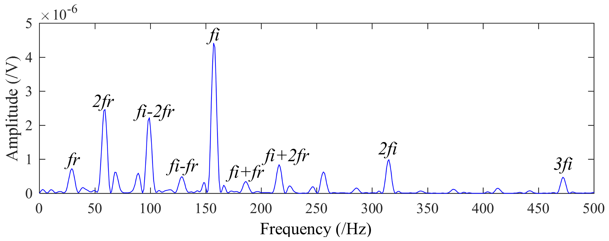
In the experiment, 12,000 data points are analyzed. Figure 16 is the time domain diagram of the fault signal of the bearing inner ring before noise reduction, where it can be seen the time domain waveform is very complex and fault feature is submerged by background noise. To minimize noise while preserving characteristics related to the fault, the multiscale local projection algorithm is used to denoise the fault signal. The time domain waveform after noise reduction is shown in Figure 17, and it can be seen that background noise of the fault signal is greatly reduced by the multiscale local projection algorithm. Figure 18, Figure 19 and Figure 20 are respectively the diagonal slice spectrum of the original signal, the frequency spectrum after noise reduction using smooth orthogonal decomposition, and the diagonal slice spectrum after noise reduction using the standard local projection algorithm. Then, the diagonal slice spectrum of signal after noise reduction is obtained as shown in Figure 21, where the rotating speed frequency f_r and its second harmonic frequency 2f_r, the inner fault frequency f_i, and the frequency multiplication 2f_i and 3f_i can be clearly observed. At the same time, both sides of the fault characteristic frequency f_i of inner ring are found to have the characteristics of the frequency band with rotation frequency as modulation frequency. The extracted features are consistent with the fault characteristics of the inner ring of the bearing, so it can be concluded that an inner ring fault occurred. It is obvious that the proposed method can extract more fault features and improve the accuracy of mechanical fault diagnosis.

4.2. Application to Drivetrain Diagnostics Simulator

To further illustrate the effectiveness of the proposed method, the faults of the gear signal and the bearing signal are simulated using the fault test bench. The experimental apparatus is shown in Figure 22, and the entire experimental device is driven by a 550 W (220 V/50 Hz) AC motor, the drive shaft is driven by the coupling, and the power is transmitted to the drive shaft of the gear box through a belt transmission. The outer ring of the replaceable rolling bearing can be treated with the method of EDM to simulate the bearing outer ring fault. The acceleration signal of the experiment is collected in the vertical direction of the bearing on the right side of the experimental platform using the CSI2130 data analyzer of America. The rolling bearing model used in the experiment was 6207E. The relevant parameters of the experiment are shown in

Table 4. Experimental parameters of rolling bearings.

Rotating Speed r (min)	Rotating Frequency fr (Hz)	Sampling Frequency (Hz)	Sampling Points	Outer Fault Frequency fo (Hz)
1450	24.17	16,384	16,380	87.01

, where the frequency f_r and the outer ring fault frequency f_o are calculated by empirical formula.

Figure 23 is the time domain diagram of the fault signal of the bearing outer ring before noise reduction, where it can be seen the time domain waveform is very complex and the fault feature is submerged by background noise. To minimize the noise while preserving the characteristics related to the fault, the multiscale local projection algorithm is used to denoise the fault signal. The time domain waveform after noise reduction is shown in Figure 24, and it can be seen the background noise of the fault signal is greatly reduced by the multiscale local projection algorithm. While Figure 25, Figure 26 and Figure 27 are respectively the diagonal slice spectrum of the original signal, the frequency spectrum after noise reduction using smooth orthogonal decomposition, and the diagonal slice spectrum after noise reduction using the standard local projection algorithm. Then, the diagonal slice spectrum of the signal after noise reduction is obtained as shown in Figure 28, where the rotating speed frequency f_r, outer fault frequency f_o, and the frequency multiplication from 2f_o to 8f_o can be clearly observed. At the same time, both sides of the fault characteristic frequency f_o of the outer ring are found to have the characteristics of the frequency band with the frequency of rotation as the modulation frequency. The extracted features are consistent with the fault characteristics of the outer ring of the bearing, so it can be judged that the bearing outer ring fault occurred. It is clear that the proposed method can extract more fault features and improve the accuracy of mechanical fault diagnosis.

The same fault simulation test bench for the above is used to collect the fault data of the gear, where the number of teeth of the gear is Z = 20, and other parameters are shown in

Table 5. Experimental parameters of gears.

Rotating Speed r (min)	Rotating Frequency fr (Hz)	Sampling Frequency (Hz)	Sampling Points	Fault Frequency f (Hz)
855	14.25	8192	8192	285

.

Figure 29 is the time domain diagram of the fault signal before noise reduction, where it can be seen the time domain waveform is very complex and the fault feature is submerged by background noise. The multiscale local projection algorithm is used to denoise the fault signal. The time domain waveform after noise reduction is shown in Figure 30, and it can be seen the background noise of the fault signal is greatly reduced by the multiscale local projection algorithm. Figure 31, Figure 32 and Figure 33 are respectively the diagonal slice spectrum of the original signal, the frequency spectrum after noise reduction using smooth orthogonal decomposition, and the diagonal slice spectrum after noise reduction using the standard local projection algorithm. In Figure 31, Figure 32 and Figure 33, although f and 3f can be found, the frequency component 2f is not extracted. Then, the diagonal slice spectrum of the signal after noise reduction is obtained as shown in Figure 34, where the fault characteristic frequency of the gear f = 285 Hz and the frequency multiplication 2f and 3f, so it can be concluded that the gear fault occurred. It is clear that the proposed method can extract more fault features, the amplitude is larger, and the fault characteristics are more obvious, which improve the accuracy of mechanical fault diagnosis.

5. Conclusions

Rolling bearings and gears work long hours in complex and harsh environments, and are susceptible to various strong noises. The fault signals often have nonstationary, nonlinear, and non-Gaussian properties, and there are a lot of secondary phase coupling phenomena. Therefore, according to the characteristics of gear and bearing fault signals, this paper presents a method of mechanical fault feature extraction based on the multiscale local projection algorithm and diagonal slice spectrum. As shown in this paper, the multiscale local projective algorithm can filter out noise while maximally preserving characteristics related to the fault, and the diagonal slice spectrum can identify the frequency components of quadratic phase coupling and enlarge coupled frequency component in the nonlinear signal. Therefore, the proposed method based on the above two algorithms can achieve more accurate results when it comes to fault feature extraction of gears and rolling bearings. The numerical simulation signal and the signal obtained from the fault simulation test bench are analyzed, and the results fully demonstrate the effectiveness and practicability of the proposed method. The extension of local projection to multiscale local projection in this paper achieves a good result based on the above researches. Aiming at further researches about local projection method, the high order polynomials can be adopted to estimate the centroid of the neighborhood. Such a strategy can preserve complete geometry of the attractors to improve noise reduction performance. The high order local projection method for fault diagnosis of rotating machinery will be conducted in future analysis.

References

1. Zhang, S.; Wang, Y.; He, S.; Jiang, Z. Bearing fault diagnosis based on variational mode decomposition and total variation denoising. Meas. Sci. Technol. 2016, 27, 075101. [Google Scholar] [CrossRef]
2. Lv, Y.; Yuan, R.; Song, G. Multivariate empirical mode decomposition and its application to fault diagnosis of rolling bearing. Mech. Syst. Sign. Proc. 2016, 81, 219–234. [Google Scholar] [CrossRef]
3. Li, K.; Su, L.; Wu, J.; Wang, H.; Chen, P. A Rolling Bearing Fault Diagnosis Method Based on Variational Mode Decomposition and an Improved Kernel Extreme Learning Machine. Appl. Sci. 2017, 7, 1004. [Google Scholar] [CrossRef]
4. Fan, Y.S.; Zheng, G.T. Research of high-resolution vibration signal detection technique and application to mechanical fault diagnosis. Mech. Syst. Sign. Proc. 2007, 21, 678–687. [Google Scholar] [CrossRef]
5. Glowacz, A.; Glowacz, W.; Glowacz, Z.; Kozik, J. Early fault diagnosis of bearing and stator faults of the single-phase induction motor using acoustic signals. Measurement 2018, 113, 1–9. [Google Scholar] [CrossRef]
6. Glowacz, A.; Glowacz, W.; Glowacz, Z. Recognition of armature current of DC generator depending on rotor speed using FFT, MSAF-1 and LDA. Eksploat. Niezawodn. 2015, 17, 64–69. [Google Scholar] [CrossRef]
7. Caesarendra, W.; Kosasih, B.; Tieu, A.K.; Moodie, C.A. Application of the largest Lyapunov exponent algorithm for feature extraction in low speed slew bearing condition monitoring. Mech. Syst. Sign. Proc. 2015, 50, 116–138. [Google Scholar] [CrossRef]
8. Chibani, A.; Chadli, M.; Peng, S.; Braiek, N.B. Fuzzy fault detection filter design for t-s fuzzy systems in finite frequency domain. IEEE Trans. Fuzzy Syst. 2017, 25, 1051–1061. [Google Scholar] [CrossRef]
9. Chadli, M.; Davoodi, M.; Meskin, N. Distributed state estimation, fault detection and isolation filter design for heterogeneous multi-agent linear parameter-varying systems. IET Contr. Theory Appl. 2016, 11, 254–262. [Google Scholar] [CrossRef]
10. Mandic, D.P.; ur Rehman, N.; Wu, Z.; Huang, N.E. Empirical mode decomposition-based time-frequency analysis of multivariate signals: The power of adaptive data analysis. IEEE Sign. Proc. Mag. 2013, 30, 74–86. [Google Scholar] [CrossRef]
11. Aguiar-Conraria, L.; Soares, M.J. The continuous wavelet transform: Moving beyond uni-and bivariate analysis. J. Econ. Surv. 2014, 28, 344–375. [Google Scholar] [CrossRef]
12. Gilles, J. Empirical wavelet transform. IEEE Trans. Sign. Proc. 2013, 61, 3999–4010. [Google Scholar] [CrossRef]
13. Zhou, B.; Liu, Z. Method of multi-resolution and effective singular value decomposition in under-determined blind source separation and its application to the fault diagnosis of roller bearing. In Proceedings of the 2015 11th International Conference on Computational Intelligence and Security (CIS), Shenzhen, China, 19–20 December 2015; pp. 462–465. [Google Scholar]
14. Cawley, R.; Hsu, G.H. Local-geometric-projection method for noise reduction in chaotic maps and flows. Phys. Rev. A 1992, 46, 3057–3082. [Google Scholar] [CrossRef] [PubMed]
15. Sauer, T. A noise reduction method for signals from nonlinear systems. Phys. D 1992, 58, 193–201. [Google Scholar] [CrossRef]
16. Kantz, H.; Schreiber, T. Nonlinear Time Series Analysis; Cambridge University Press: Cambridge, UK, 2003. [Google Scholar]
17. Cao, L. Practical method for determining the minimum embedding dimension of a scalar time series. Phys. D Nonlinear Phenom. 1997, 110, 43–50. [Google Scholar] [CrossRef]
18. Wang, G.F.; Li, Y.B.; Luo, Z.G. Fault classification of rolling bearing based on reconstructed phase space and Gaussian mixture model. J. Sound Vib. 2009, 323, 1077–1089. [Google Scholar] [CrossRef]
19. Vautard, R.; Yiou, P.; Ghil, M. Singular-spectrum analysis: A toolkit for short, noisy chaotic signals. Phys. D Nonlinear Phenom. 1992, 58, 95–126. [Google Scholar] [CrossRef]
20. Lv, Y.; He, B.; Yi, C.; Dang, Z. 2366. A novel scheme on multi-channel mechanical fault signal diagnosis based on augmented quaternion singular spectrum analysis. J. Vibroeng. 2017, 19, 955–966. [Google Scholar]
21. Michael, T.J.; Richard, J.P. Generalized phase space projection for nonlinear noise reduction. Phys. D 2005, 201, 306–317. [Google Scholar]
22. Jevtić, N.; Stine, P.; Schweitzer, J.S. Nonlinear time series analysis of Kepler Space Telescope data: Mutually beneficial progress. Astron. Nachr. 2012, 333, 983–986. [Google Scholar] [CrossRef]
23. Kotas, M. Projective filtering of time warped ECG beats. Comp. Biol. Med. 2008, 38, 127–137. [Google Scholar] [CrossRef] [PubMed]
24. Grassberger, P.; Schreiber, T.; Schaffrath, C. Nonlinear time sequence analysis. Int. J. Bifurc. Chaos 1991, 1, 521–547. [Google Scholar] [CrossRef]
25. Grassberger, P.; Hegger, R.; Kantz, H.; Schaffrath, C.; Schreiber, T. On noise reduction methods for chaotic data. Chaos: An Interdisciplinary. J. Nonlinear Sci. 1993, 3, 127–141. [Google Scholar]
26. Chelidze, D. Smooth local subspace projection for nonlinear noise reduction. Chaos Interdiscip. J. Nonlinear Sci. 2014, 24, 013121. [Google Scholar] [CrossRef] [PubMed]
27. Moore, J.M.; Small, M.; Karrech, A. Improvements to local projective noise reduction through higher order and multiscale refinements. Chaos Interdiscip. J. Nonlinear Sci. 2015, 25, 063114. [Google Scholar] [CrossRef] [PubMed]
28. Tugnait, J.K.; Luo, W. On channel estimation using superimposed training and first-order statistics. In Proceedings of the 2003 IEEE International Conference on Acoustics, Speech, and Signal Processing, Hong Kong, China, 6–10 April 2003; Volume 4. [Google Scholar]
29. Tong, L.; Xu, G.; Kailath, T. Blind Identification and equalisation based on second-order statistics: A time domain approach. IEEE Trans. Inf. Theory 1994, 40, 340–349. [Google Scholar] [CrossRef]
30. Rosa, J.; Lloret, I.; Puntonet, C.G.; Piotrkowski, R.; Moreno, A. Higher-order spectra measurement techniques of termite emissions. A characterization framework. Measurement 2008, 41, 105–118. [Google Scholar] [CrossRef]
31. Chua, K.C.; Chandran, V.; Acharya, U.R.; Lim, C.M. Application of higher order statistics/spectra in biomedical signals—A review. Med. Eng. Phys. 2010, 32, 679–689. [Google Scholar] [CrossRef] [PubMed] [Green Version]
32. Zheng, K.; Li, T.; Zhang, B.; Zhang, Y.; Luo, J.; Zhou, X. Incipient Fault Feature Extraction of Rolling Bearings Using Autocorrelation Function Impulse Harmonic to Noise Ratio Index Based SVD and Teager Energy Operator. Appl. Sci. 2017, 7, 1117. [Google Scholar] [CrossRef]
33. Jiang, Z.; Hu, M.; Feng, K.; He, Y. Weak fault feature extraction scheme for intershaft bearings based on linear prediction and order tracking in the rotation speed difference domain. Appl. Sci. 2017, 7, 937. [Google Scholar] [CrossRef]
34. Loparo, K.A. Bearings Vibration Data Set, Case Western Reserve University. Available online: http://csegroups.case.edu/bearingdatacenter/home (accessed on 30 October 2017).
35. Mendel, J.M. Tutorial on higher-order statistics (spectra) in signal processing and system theory: Theoretical results and some applications. Proc. IEEE 1991, 79, 278–305. [Google Scholar] [CrossRef]
36. Nikias, C.L.; Mendel, J.M. Signal processing with higher-order spectra. IEEE Sign. Proc. Mag. 1993, 10, 10–37. [Google Scholar] [CrossRef]
Figure 1. Schematic diagram of local linear approximations.
Applsci 08 00619 g001
Figure 2. Improved method by Sauer [15].
Applsci 08 00619 g002
Figure 3. Normalized expectation error. β: scale factor; T(β): error.
Applsci 08 00619 g003
Figure 4. Local enlargement of normalized expectation error.
Applsci 08 00619 g004
Figure 5. The proposed fault diagnosis scheme of rotating machinery based on the multiscale local projection method and diagonal slice spectrum.
Applsci 08 00619 g005
Figure 6. Time domain plot of Lorenz without noise.
Applsci 08 00619 g006
Figure 7. Time domain plot of Lorenz with noise.
Applsci 08 00619 g007
Figure 8. Time domain plot of Lorenz after noise reduction.
Applsci 08 00619 g008
Figure 9. Local enlargement of time domain plot after noise reduction.
Applsci 08 00619 g009
Figure 10. (a) Phase diagram of Lorenz without noise. (b) Phase diagram of Lorenz with noise. (c) Phase diagram of Lorenz after noise reduction by the standard local projection algorithm. (d) Phase diagram of Lorenz after noise reduction by multiscale local projection. (τ = 1)
Applsci 08 00619 g010
Figure 11. Diagonal slice spectrum of original signal.
Applsci 08 00619 g011
Figure 12. Diagonal slice spectrum of noisy signal.
Applsci 08 00619 g012
Figure 13. Diagonal slice spectrum after using standard local projection for noise reduction.
Applsci 08 00619 g013
Figure 14. Diagonal slice spectrum after using multiscale local projection for noise reduction.
Applsci 08 00619 g014
Figure 15. Rolling bearing fault simulator. 1, 3-Hp motor, 2-Torque transducer and encoder
Applsci 08 00619 g015
Figure 16. The time waveform of the original signal with an inner race defect.
Applsci 08 00619 g016
Figure 17. The time waveform after noise reduction.
Applsci 08 00619 g017
Figure 18. The diagonal slice spectrum of the original signal.
Applsci 08 00619 g018
Figure 19. The frequency spectrum after noise reduction using smooth orthogonal decomposition.
Applsci 08 00619 g019
Figure 20. The diagonal slice spectrum after noise reduction using standard local projection.
Applsci 08 00619 g020
Figure 21. The diagonal slice spectrum after noise reduction using multiscale local projection.
Applsci 08 00619 g021
Figure 22. Fault simulation device for rolling bearing and gear. 1—motor, 2—coupler, 3—replaceable rolling bearing with 6207, 4—belt pulley, 5—device box, 6—transmission shaft, 7—gear.
Applsci 08 00619 g022
Figure 23. The time waveform of the original signal with an outer race defect.
Applsci 08 00619 g023
Figure 24. The time waveform after noise reduction.
Applsci 08 00619 g024
Figure 25. The diagonal slice spectrum of the original signal.
Applsci 08 00619 g025
Figure 26. The frequency spectrum after noise reduction using smooth orthogonal decomposition.
Applsci 08 00619 g026
Figure 27. The diagonal slice spectrum after noise reduction using standard local projection.
Applsci 08 00619 g027
Figure 28. The diagonal slice spectrum after noise reduction using multiscale local projection.
Applsci 08 00619 g028
Figure 29. The time waveform of the original signal.
Applsci 08 00619 g029
Figure 30. The time waveform after noise reduction.
Applsci 08 00619 g030
Figure 31. The diagonal slice spectrum of the original signal.
Applsci 08 00619 g031
Figure 32. The frequency spectrum after noise reduction using smooth orthogonal decomposition.
Applsci 08 00619 g032
Figure 33. The diagonal slice spectrum after noise reduction using standard local projection.
Applsci 08 00619 g033
Figure 34. The diagonal slice spectrum after noise reduction using multiscale local projection.
Applsci 08 00619 g034