Forecasting of Power Grid Investment in China Based on Support Vector Machine Optimized by Differential Evolution Algorithm and Grey Wolf Optimization Algorithm

Abstract

In recent years, the construction of China’s power grid has experienced rapid development, and its scale has leaped into the first place in the world. Accurate and effective prediction of power grid investment can not only help pool funds and rationally arrange investment in power grid construction, but also reduce capital costs and economic risks, which plays a crucial role in promoting power grid investment planning and construction process. In order to forecast the power grid investment of China accurately, firstly on the basis of analyzing the influencing factors of power grid investment, the influencing factors system for China’s power grid investment forecasting is constructed in this article. The method of grey relational analysis is used for screening the main influencing factors as the prediction model input. Then, a novel power grid investment prediction model based on DE-GWO-SVM (support vector machine optimized by differential evolution and grey wolf optimization) algorithm is proposed. Next, two cases are taken for empirical analysis to prove that the DE-GWO-SVM model has strong generalization capacity and has achieved a good prediction effect for power grid investment forecasting in China. Finally, the DE-GWO-SVM model is adopted to forecast power grid investment in China from 2018 to 2022.

1. Introduction

Presently, for social development, the power grid plays a crucial role which shoulders the important responsibilities of optimizing the allocation of energy resources and promoting social development, and it is the major implementation body of energy strategy. In recent years, the construction of China’s power grid has experienced rapid development, and its scale has leaped into the first place in the world. From 2016–2020, the investment scale of the power industry in China is planned to reach 7170 billion yuan, of which 3830 billion yuan will be invested in power generation and 3340 billion yuan in power grid investment. Accurate and effective prediction of power grid investment can not only help pool funds and rationally arrange investment in power grid construction, but also reduce capital costs and economic risks, which plays a crucial role in promoting power grid investment planning and construction process.

Recently, scholars have applied a variety of forecasting models—such as error correction model, autoregressive integrated moving average model, and grey model—to predict the investment in various fields, and have obtained some achievements. The error correction model is a specific econometric model, which was put forward by Davidson et al. in 1978 [1]. Through cointegration analysis of variables, the long-term equilibrium relationship among variables is found out to form an error correction term. The error correction term is taken as an explanatory variable, then the short-term model is established, namely the error correction model [2,3]. The autoregressive integrated moving average model is a well-known time series prediction method first proposed by Box and Jenkins in the early 1970s [4]. It transforms a nonstationary time series into a stationary time series, and then uses the lag value of the dependent variable and the present value and the lag value of the random error term as the independent variables to construct the regression model [5]. The grey model can make fuzzy long-term description of the law of things development through establishing the grey differential prediction model with a small amount of incomplete information [6]. The model of GM(1,1) is the most commonly applied grey model, which consists of a first order differential equation containing only one variable. The model is simple to calculate and has obvious advantages for the forecasting of small sample data with irregular distribution [7,8]. Lunsford [9] proposed an error correction model based on the stock–flow relationship of housing unit start, construction, and completion to predict housing investment in the United States. Singh et al. [10] collected the air traffic data, gross domestic product, and industrial production index of the India civil aviation department to study the corresponding elasticity coefficient, and predicted the capacity demand and investment demand of India airport infrastructure for the next 20 years. Chang and Linneman [11] used the time series model to forecast the growth rate of real estate investment in other countries on the basis of studying the substitution model of real estate investment growth rates in Japan, Korea, Taiwan, and the United States. Gupta [12] proposed a Bayesian vector error correction model to predict South Africa’s inventory investment based on the quarterly data of actual sales, output, undelivered orders, price level, and interest rate. Jere et al. [13] used the simple exponential smoothing method, the three exponential smoothing method, and the autoregressive moving average method to predict the annual foreign direct investment in Zambia. By error comparison, the autoregressive moving average method was proved to be the most suitable model. However, so far, less research results have been achieved by scholars in the study of power grid investment forecasting. Zhao et al. [14] proposed a forecasting model for power grid investment using cointegration theory and error correction model. Through screening variables by augmented dickey-fuller (ADF) unit root test and Johansen cointegration test, a long-term equilibrium model between grid investment and maximum electricity load was established, and a short-term regulation relation model was constructed by error correction model for improving prediction accuracy. Hu et al. [15] studied a calculation model of power grid infrastructure investment by grey theory. On the basis of establishing the forecasting index system for power grid infrastructure investment and predicting the indicators by grey theory, the power grid infrastructure investment forecasting model was established by determining the impact of the changes of measurement indexes on power grid infrastructure investment through analytic hierarchy process (AHP). Fang et al. [16] used the grey prediction method and hierarchical analysis method to construct the power grid investment forecasting model by analysis of the main influencing factors. To sum up, there are relatively few research results on power grid investment prediction, and the prediction models used by the researchers are relatively traditional, such as time series model, grey model, error correction model, and so on.

Artificial intelligence, also known as machine intelligence, is a novel technology for researching the theory, method, and application systems for simulating human intelligence [17,18]. Artificial intelligence is a major achievement in computer science development in the 20th century [19,20]. It has seen widespread use in many fields, such as prediction. Compared with classic prediction technologies, artificial intelligence prediction technology has shown strong superiority in prediction accuracy. Neural network [21,22,23] and support vector machine (SVM) [24,25,26] are two typical and widely used artificial intelligence prediction techniques. However, compared with neural networks, support vector machine developed in the statistical learning theory has a more solid foundation of mathematical theory, which can effectively solve the high-dimensional data model construction problems under the condition of limited samples. It has become one of the most popular research directions in the machine learning field with a stronger generalization ability. For further improving the prediction performance of SVM, researchers have used various algorithms to optimize SVM parameters, such as fruit fly optimization [27,28,29], particle swarm optimization [30,31], genetic algorithm [32,33,34], whale optimization algorithm [35,36], and so on. In this article, grey wolf optimization improved by differential evolution is adopted to optimize SVM parameters. The differential evolution (DE) [37,38] was first proposed by Storn and Price in 1995, which is mainly used to solve real number optimization problems. The algorithm is a group based adaptive global optimization algorithm, which belongs to one of the evolutionary algorithms. It has the characteristics of simple structure, easy implementation, fast convergence, and strong robustness [39]. The differential evolution algorithm was proved to be the fastest evolutionary algorithm in the first international evolutionary computation competition in Nagoya, Japan, 1996. Grey wolf optimization (GWO) algorithm [40,41] is a novel algorithm for guiding the group to search the optimal value, which is inspired by wolves’ hunting behavior and social hierarchy. It has obvious advantages in global search and convergence [42]. Jin et al. [43] proposed a hybrid optimization method using differential evolution and grey wolf optimization. Through three simulation experiments, it was proven that the hybrid optimization algorithm had improved the solving precision, convergence speed, and search ability compared with a single algorithm. Xu and Ding [44] proposed a short-term cloud computing resource load forecasting model using grey wolf optimization and support vector machine, which could accurately describe the complex trend of the short-term cloud computing resource loads and effectively improve the prediction accuracy of the short-term cloud computing resource loads. In this article, the three algorithms of differential evolution algorithm, grey wolf optimization algorithm, and support vector machine are combined for power grid investment forecasting. The improved combination prediction model will greatly improve the global search capability for avoiding falling into the local optimum.

In this article, for forecasting the power grid investment of China accurately, based on the construction of influencing factors system for power grid investment forecasting, a novel power grid investment prediction model based on DE-GWO-SVM algorithm is proposed in this article. The innovations of this article are as follows:

(1)

Power grid investment forecasting in China is affected by many factors. In order to realize the accurate forecasting of China’s power grid investment, relevant factors of power grid investment forecasting are preliminarily selected based on studying a large number of literatures in this article. Through the Delphi method, multiple rounds of anonymous consultations and feedbacks are carried out on experts’ opinions, and the influencing factors system for China’s power grid investment forecasting is finally determined. From the four dimensions of economic development, electricity demand, power grid scale, and power grid benefit, the influencing factors system for power grid investment forecasting is constructed. Then, the method of grey relational analysis is used for screening the main influencing factors of power grid investment as the prediction model input.

(2)

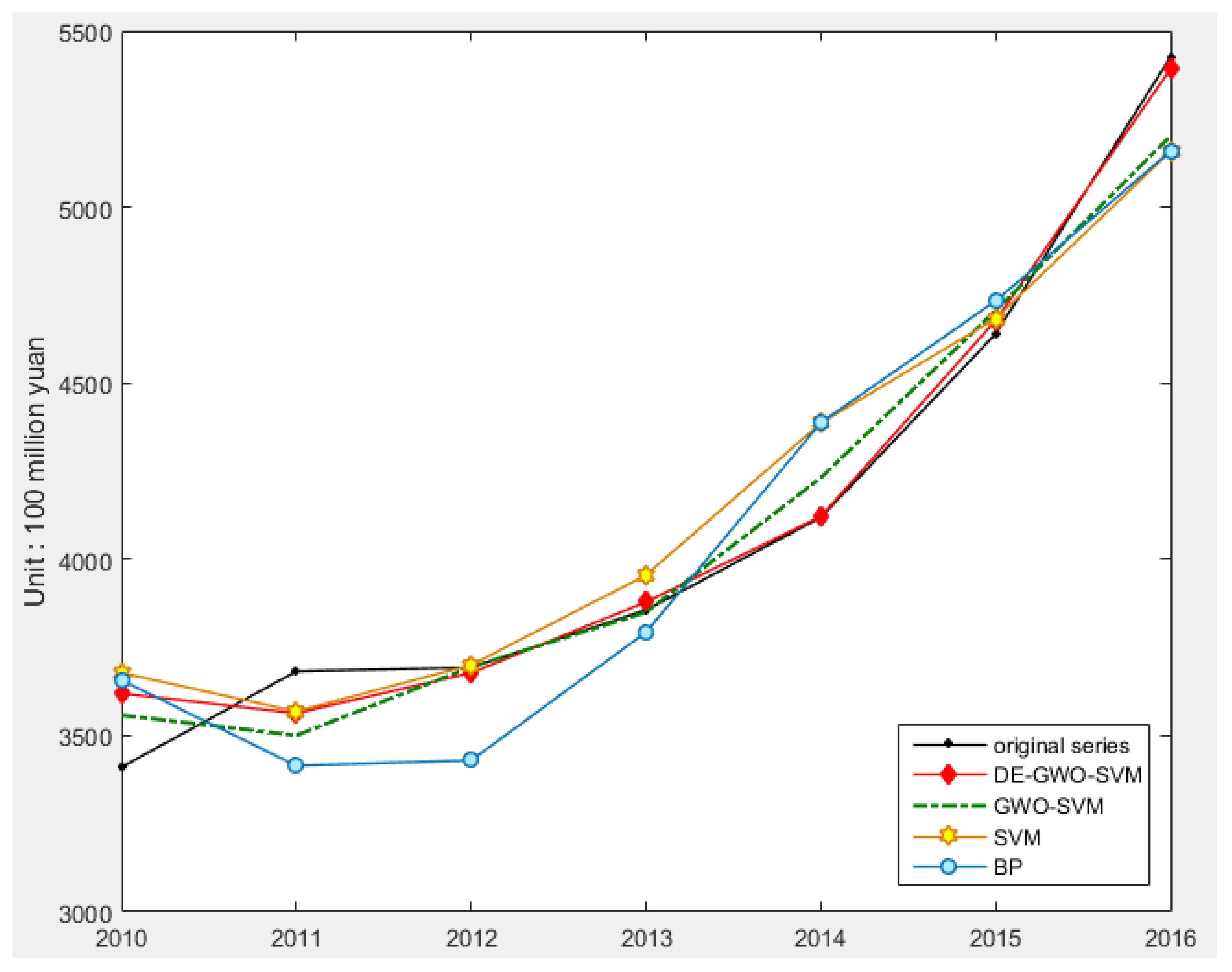
In this article, the model of DE-GWO-SVM is proposed to predict power grid investment in China. Three algorithms—differential evolution algorithm, grey wolf optimization algorithm, and support vector machine—are combined for power grid investment forecasting. The improved combination prediction model will greatly improve the global search capability for avoiding being lost into the local optimum, which can predict the power grid investment accurately. Through empirical analysis, it is proven that the DE-GWO-SVM model has strong generalization ability and robustness in power grid investment prediction, whose prediction accuracy is better than that of GWO-SVM, SVM, and back propagation (BP) neural network.

The main structure of this article is arranged as follows: Section 2 introduces the methodology, including establishing the influencing factors system for power grid investment forecasting, introducing grey relational analysis which is used for the main influencing factors screening, and proposing the DE-GWO-SVM forecasting model. Section 3 carries out empirical analysis to verify the validity of the proposed model for the power grid investment prediction in China, and forecasts the power grid investment in China from 2018 to 2022. Section 4 summarizes the whole article.

2. Methodology

2.1. Construction of the Influencing Factors System for Power Grid Investment Forecasting

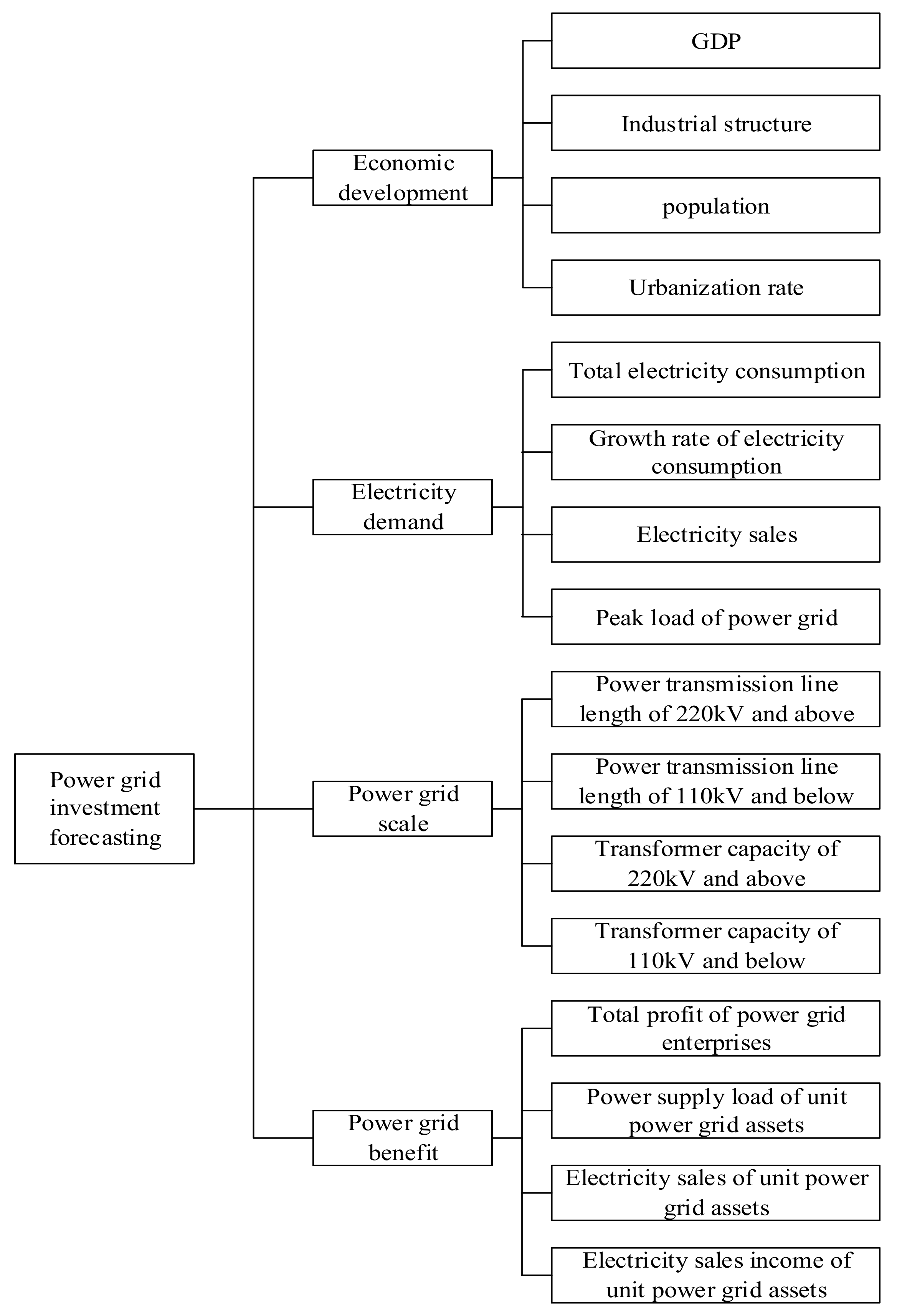
Power grid investment forecasting in China is affected by many factors. In order to realize the accurate forecasting of China’s power grid investment, relevant factors of power grid investment forecasting are preliminarily selected based on studying a large number of literatures in this article. Through the Delphi method, multiple rounds of anonymous consultations and feedbacks are carried out on experts’ opinions, and the influencing factors system for China’s power grid investment forecasting is finally determined. The influencing factors system for power grid investment forecasting is constructed from the four dimensions of economic development, electricity demand, power grid scale, and power grid benefit and each dimension contains four factors. So, there are 16 influencing factors in the influencing factors system. They are gross domestic product (GDP), industrial structure (the proportion of the third industry added value), population, urbanization rate, total electricity consumption, growth rate of electricity consumption, electricity sales, peak load of power grid, power transmission line length of 220 kV and above, power transmission line length of 110 kV and below, transformer capacity of 220 kV and above, transformer capacity of 110 kV and below, total profit of power grid enterprises, power supply load of unit power grid assets, electricity sales of unit power grid assets, and electricity sales income of unit power grid assets. The influencing factors system for power grid investment forecasting is shown in Figure 1.

2.2. Screening of the Main Influencing Factors Based on Grey Relational Analysis

The relational degree is the degree of relevance between two things. In mathematics, it is a term for grey system analysis and refers to the degree of similarity between two functions. The calculation of grey relational degree is the core of grey relational analysis [45,46,47]. In the process of system development, if the trend of two factors is consistent—that is, the degree of synchronous change is relatively high—it can be said that the relational degree between the two factors is relatively high. Otherwise, it is relatively low. Therefore, grey relational analysis is a method to measure the relational degree among factors according to the similarity or dissimilarity degree of development trends of them. In this paper, grey relational analysis is used to screen influencing factors for power grid investment forecasting. By calculating grey relational degrees between the above 16 influencing factors and power grid investment, the main influencing factors are sorted and screened out, and the selected factors are used as the input of the forecasting model.

The specific steps for calculating the grey relational degree are as follows:

(1) Determine the analysis sequences.

The time sequences of power grid investment is set as

$${\mathrm{X}}_0=({\mathrm{x}}_0(1),{\mathrm{x}}_0(2),\cdots ,{\mathrm{x}}_0(\mathrm{n}))$$

(1)

The time sequences of various influencing factors are set as

$$\{\begin{array}{c}{\mathrm{X}}_1=({\mathrm{x}}_1(1),{\mathrm{x}}_1(2),\cdots ,{\mathrm{x}}_1(\mathrm{n}))\\ {\mathrm{X}}_2=({\mathrm{x}}_2(1),{\mathrm{x}}_2(2),\cdots ,{\mathrm{x}}_2(\mathrm{n}))\\ \cdots \\ {\mathrm{X}}_{\mathrm{m}}=({\mathrm{x}}_{\mathrm{m}}(1),{\mathrm{x}}_{\mathrm{m}}(2),\cdots ,{\mathrm{x}}_{\mathrm{m}}(\mathrm{n}))\end{array}$$

(2)

(2) Do non-dimensional processing on each sequence.

$$\begin{gathered} {\mathrm{y}}_{\mathrm{i}}(\mathrm{k})=\frac{{\mathrm{x}}_{\mathrm{i}}(\mathrm{k})}{\frac{1}{\mathrm{n}}{\displaystyle \sum _{\mathrm{k}=1}^{\mathrm{n}}{\mathrm{x}}_{\mathrm{i}}(\mathrm{k})}} \\ \mathrm{k}=1,2,\cdots ,\mathrm{n}, \mathrm{i}=0,1,2,\cdots ,\mathrm{m} \end{gathered}$$

(3)

(3) Calculate the relational coefficient.

The relational coefficient between ${\mathrm{y}}_{\mathrm{j}}(\mathrm{k})$ and ${\mathrm{y}}_0(\mathrm{k})$ is shown as

$$\begin{gathered} {\mathsf{\xi }}_{\mathrm{j}}(\mathrm{k})=\frac{\underset{\mathrm{j}}{\min }\underset{\mathrm{k}}{\min }\left|{\mathrm{y}}_0(\mathrm{k})-{\mathrm{y}}_{\mathrm{j}}(\mathrm{k})\right|+\mathsf{\rho }\underset{\mathrm{j}}{\max }\underset{\mathrm{k}}{\max }\left|{\mathrm{y}}_0(\mathrm{k})-{\mathrm{y}}_{\mathrm{j}}(\mathrm{k})\right|}{\left|{\mathrm{y}}_0(\mathrm{k})-{\mathrm{y}}_{\mathrm{j}}(\mathrm{k})\right|+\mathsf{\rho }\underset{\mathrm{j}}{\max }\underset{\mathrm{k}}{\max }\left|{\mathrm{y}}_0(\mathrm{k})-{\mathrm{y}}_{\mathrm{j}}(\mathrm{k})\right|} \\ \mathsf{\rho }\in (0,1),\mathrm{k}=1,2,\cdots ,\mathrm{n}, \mathrm{j}=1,2,\cdots ,\mathrm{m} \end{gathered}$$

(4)

(4) Calculate the relational degree.

The grey relational degree between ${\mathrm{X}}_{\mathrm{j}}$ and ${\mathrm{X}}_0$ is shown as

$$\begin{gathered} {\mathrm{r}}_{\mathrm{j}}=\frac{1}{\mathrm{n}}{\displaystyle \sum _{\mathrm{k}=1}^{\mathrm{n}}{\mathsf{\xi }}_{\mathrm{j}}(\mathrm{k})} \\ \mathrm{k}=1,2,\cdots ,\mathrm{n}, \mathrm{j}=1,2,\cdots ,\mathrm{m} \end{gathered}$$

(5)

(5) Conduct relational degrees sorting.

The influencing factors sequences are sorted according to the grey relational degrees. The greater the grey relational degree is, the more consistent the influencing factor sequence is with the power grid investment sequence, and the closer the link between the influencing factor and the power grid investment is.

2.3. Support Vector Machine

Support vector machine is proposed by Vapnik et al. It is a small sample machine learning method on the basis of VC dimension theory [24,25]. The basic idea of using the SVM algorithm to estimate the regression function is to nonlinearly map data to a high-dimensional feature space, and then carry out linear regression in this high-dimensional space [26].

Set $\mathrm{n}$ training sample sets: $\left\{({\mathrm{x}}_{\mathrm{i}},{\mathrm{y}}_{\mathrm{i}})|\mathrm{i}=1,2,\cdots ,\mathrm{n}\right\}$. Among them, ${\mathrm{x}}_{\mathrm{i}}\in {\mathrm{R}}^{\mathrm{d}}$ are training sample inputs of $\mathrm{d}$ dimension, ${\mathrm{y}}_{\mathrm{i}}\in \mathrm{R}$ are training sample outputs. The nonlinear mapping $\mathsf{\psi }(\mathrm{x})=(\mathsf{\phi }({\mathrm{x}}_1),\mathsf{\phi }({\mathrm{x}}_2),\cdots ,\mathsf{\phi }({\mathrm{x}}_{\mathrm{n}}))$ is used to map input samples from the original space ${\mathrm{R}}^{\mathrm{d}}$ to the high-dimensional feature space ${\mathrm{R}}^{\mathrm{k}}(\mathrm{k}>\mathrm{d})$. The optimal linear regression function is constructed in the high-dimensional feature space

$$\mathrm{f}({\mathrm{x}}_{\mathrm{i}})={\mathsf{\omega }}^{\mathrm{T}}\mathsf{\phi }({\mathrm{x}}_{\mathrm{i}})+\mathrm{b}$$

(6)

In the equation: $\mathsf{\omega }$ is the weight vector in the high-dimensional feature space, $\mathsf{\omega }\in {\mathrm{R}}^{\mathrm{k}}$. $\mathrm{b}$ is the bias constant, $\mathrm{b}\in \mathrm{R}$.

Determine $\mathsf{\omega }$ and $\mathrm{b}$ in the light of the principle of structural risk minimization

$$\min \mathrm{R}=\frac{1}{2}{\Vert \mathsf{\omega }\Vert }^2+\mathrm{c}\cdot {\mathrm{R}}_{\mathrm{e}\mathrm{m}\mathrm{p}}$$

(7)

In the equation, ${\Vert \mathsf{\omega }\Vert }^2$ controls the model complexity, $\mathrm{c}$ is the regularization parameter and ${\mathrm{R}}_{\mathrm{e}\mathrm{m}\mathrm{p}}$ is the error control function. If ${\mathrm{R}}_{\mathrm{e}\mathrm{m}\mathrm{p}}$ selects different loss functions, different forms of SVM can be constructed. The loss function of standard SVM in the optimization objective is the linear term of the error.

In the light of the principle of structural risk minimization, Equation (7) can be transformed into

$$\begin{array}{l}\min \mathrm{J}=\frac{1}{2}{\Vert \mathsf{\omega }\Vert }^2+\mathrm{c}{\displaystyle \sum _{\mathrm{i}=1}^{\mathrm{n}}({\mathsf{\xi }}_{\mathrm{i}}+{\mathsf{\xi }}_{\mathrm{i}}{}^{\ast })}\\ \mathrm{s}.\mathrm{t}.\{\begin{array}{c}{\mathrm{y}}_{\mathrm{i}}-{\mathsf{\omega }}^{\mathrm{T}}\mathsf{\phi }({\mathrm{x}}_{\mathrm{i}})-\mathrm{b}\le \mathsf{\epsilon }+{\mathsf{\xi }}_{\mathrm{i}}\\ {\mathsf{\omega }}^{\mathrm{T}}\mathsf{\phi }({\mathrm{x}}_{\mathrm{i}})+\mathrm{b}-{\mathrm{y}}_{\mathrm{i}}\le \mathsf{\epsilon }+{\mathsf{\xi }}_{\mathrm{i}}\\ {\mathsf{\xi }}_{\mathrm{i}},{\mathsf{\xi }}_{\mathrm{i}}{}^{\ast }\ge 0 (\mathrm{i}=1,2,\cdots ,\mathrm{n})\end{array}\end{array}$$

(8)

In the equation, $\mathsf{\epsilon }$ is the insensitivity coefficient, ${\mathsf{\xi }}_{\mathrm{i}}$ and ${\mathsf{\xi }}_{\mathrm{i}}{}^{\ast }$ are relaxation factors.

Solve optimization problem with Lagrange function,

$$\begin{array}{ll}\mathrm{L}(\mathsf{\omega },{\mathsf{\xi }}_{\mathrm{i}},{\mathsf{\xi }}_{\mathrm{i}}{}^{\ast },\mathsf{\alpha },{\mathsf{\alpha }}^{\ast },\mathrm{c},\mathsf{\beta },{\mathsf{\beta }}^{\ast })=\frac{1}{2}& {\Vert \mathsf{\omega }\Vert }^2+\mathrm{c}{\displaystyle \sum _{\mathrm{i}=1}^{\mathrm{n}}({\mathsf{\xi }}_{\mathrm{i}}+{\mathsf{\xi }}_{\mathrm{i}}{}^{\ast })}\\ & -{\displaystyle \sum _{\mathrm{i}=1}^{\mathrm{n}}{\mathsf{\alpha }}_{\mathrm{i}}\left[{\mathsf{\omega }}^{\mathrm{T}}\mathsf{\phi }({\mathrm{x}}_{\mathrm{i}})+\mathrm{b}-{\mathrm{y}}_{\mathrm{i}}+\mathsf{\epsilon }+{\mathsf{\xi }}_{\mathrm{i}}\right]}\\ & -{\displaystyle \sum _{\mathrm{i}=1}^{\mathrm{n}}{\mathsf{\alpha }}_{\mathrm{i}}{}^{\ast }\left[{\mathrm{y}}_{\mathrm{i}}-{\mathsf{\omega }}^{\mathrm{T}}\mathsf{\phi }({\mathrm{x}}_{\mathrm{i}})-\mathrm{b}+\mathsf{\epsilon }+{\mathsf{\xi }}_{\mathrm{i}}{}^{\ast }\right]}\\ & -{\displaystyle \sum _{\mathrm{i}=1}^{\mathrm{n}}({\mathsf{\beta }}_{\mathrm{i}}{\mathsf{\xi }}_{\mathrm{i}}+{\mathsf{\beta }}_{\mathrm{i}}{}^{\ast }{\mathsf{\xi }}_{\mathrm{i}}{}^{\ast })}\end{array}$$

(9)

In the equation, ${\mathsf{\alpha }}_{\mathrm{i}}, {\mathsf{\alpha }}_{\mathrm{i}}{}^{\ast }, {\mathsf{\beta }}_{\mathrm{i}}, {\mathsf{\beta }}_{\mathrm{i}}{}^{\ast }$ are all Lagrange multipliers and ${\mathsf{\alpha }}_{\mathrm{i}}>0, {\mathsf{\alpha }}_{\mathrm{i}}{}^{\ast }>0, {\mathsf{\beta }}_{\mathrm{i}}>0, {\mathsf{\beta }}_{\mathrm{i}}{}^{\ast }>0 (\mathrm{i}=1,2,\cdots ,\mathrm{n})$.

According to Karush–Kuhn–Tucker optimization condition,

$$\{\begin{array}{l}\frac{\partial \mathrm{L}}{\partial \mathsf{\omega }}=0\to \mathsf{\omega }={\displaystyle \sum _{\mathrm{i}=1}^{\mathrm{n}}({\mathsf{\alpha }}_{\mathrm{i}}-{\mathsf{\alpha }}_{\mathrm{i}}{}^{\ast })\mathsf{\phi }({\mathrm{x}}_{\mathrm{i}})}\\ \frac{\partial \mathrm{L}}{\partial \mathrm{b}}=0\to {\displaystyle \sum _{\mathrm{i}=1}^{\mathrm{n}}({\mathsf{\alpha }}_{\mathrm{i}}-{\mathsf{\alpha }}_{\mathrm{i}}{}^{\ast })=0}\\ \frac{\partial \mathrm{L}}{\partial {\mathsf{\xi }}_{\mathrm{i}}}=0\to \mathrm{c}-{\mathsf{\alpha }}_{\mathrm{i}}-{\mathsf{\beta }}_{\mathrm{i}}=0\\ \frac{\partial \mathrm{L}}{\partial {\mathsf{\xi }}_{\mathrm{i}}{}^{\ast }}=0\to \mathrm{c}-{\mathsf{\alpha }}_{\mathrm{i}}{}^{\ast }-{\mathsf{\beta }}_{\mathrm{i}}{}^{\ast }=0\end{array}$$

(10)

Define $\mathrm{K}({\mathrm{x}}_{\mathrm{i}},{\mathrm{x}}_{\mathrm{j}})=\mathsf{\phi }{({\mathrm{x}}_{\mathrm{i}})}^{\mathrm{T}}\mathsf{\phi }({\mathrm{x}}_{\mathrm{j}})$ as the symmetric kernel function of the Mercer condition. Then the optimization problem can be expressed as:

$$\begin{array}{ll}\max \mathrm{W}(\mathsf{\alpha },{\mathsf{\alpha }}^{\ast })=& -\frac{1}{2}{\displaystyle \sum _{\mathrm{i},\mathrm{j}=1}^{\mathrm{n}}({\mathrm{a}}_{\mathrm{i}}-{\mathrm{a}}_{\mathrm{i}}{}^{\ast })}({\mathrm{a}}_{\mathrm{j}}-{\mathrm{a}}_{\mathrm{j}}{}^{\ast })\mathrm{K}({\mathrm{x}}_{\mathrm{i}},{\mathrm{x}}_{\mathrm{j}})\hfill \\ & +{\displaystyle \sum _{\mathrm{i}=1}^{\mathrm{n}}({\mathrm{a}}_{\mathrm{i}}-{\mathrm{a}}_{\mathrm{i}}{}^{\ast })}{\mathrm{y}}_{\mathrm{i}}-{\displaystyle \sum _{\mathrm{i}=1}^{\mathrm{n}}({\mathrm{a}}_{\mathrm{i}}-{\mathrm{a}}_{\mathrm{i}}{}^{\ast })}\mathsf{\epsilon }\hfill \\ \mathrm{s}.\mathrm{t}.\{\begin{array}{c}{\displaystyle \sum _{\mathrm{i}=1}^{\mathrm{n}}({\mathrm{a}}_{\mathrm{i}}-{\mathrm{a}}_{\mathrm{i}}{}^{\ast })}=0\\ 0\le {\mathrm{a}}_{\mathrm{i}},{\mathrm{a}}_{\mathrm{i}}{}^{\ast }\le \mathrm{c}\end{array}& \end{array}$$

(11)

The nonlinear forecasting model can be obtained:

$$\mathrm{f}(\mathrm{x})={\displaystyle \sum _{\mathrm{i}=1}^{\mathrm{n}}({\mathsf{\alpha }}_{\mathrm{i}}-{\mathsf{\alpha }}_{\mathrm{i}}{}^{\ast })\mathrm{K}({\mathrm{x}}_{\mathrm{i}},{\mathrm{x}}_{\mathrm{j}})}+\mathrm{b}$$

(12)

In this article, the radial basis kernel function is selected as the kernel function of SVM, which is defined as:

$$\mathrm{K}({\mathrm{x}}_{\mathrm{i}},{\mathrm{x}}_{\mathrm{j}})=\exp \left(\frac{-{\Vert {\mathrm{x}}_{\mathrm{i}}-{\mathrm{x}}_{\mathrm{j}}\Vert }^2}{2{\sigma }^2}\right)$$

(13)

In the equation, $\sigma$ is the width parameter of radial basis kernel function.

2.4. Grey Wolf Optimization

Grey wolf optimization (GWO) algorithm is a novel heuristic swarm intelligence optimization algorithm proposed by Mirjalili et al. in 2014, which has good performance in global search and convergence [40]. GWO simulates the social hierarchy and hunting behavior of the grey wolf population [41,42]. The grey wolf population in nature is divided into four grades: $\mathsf{\alpha }$, $\mathsf{\beta }$, $\mathsf{\delta }$, and $\mathsf{\omega }$, in order of social status from high to low. Define the current optimum solution in the wolf population as $\mathsf{\alpha }$ wolf, the second-best solution as $\mathsf{\beta }$ wolf, the third-best solution as $\mathsf{\delta }$ wolf, and other solutions as $\mathsf{\omega }$ wolf to construct the hierarchy model of the grey wolf. In the GWO algorithm, the hunting task is performed by $\mathsf{\alpha }$, $\mathsf{\beta }$, and $\mathsf{\delta }$ wolf. $\mathsf{\omega }$ wolf follows the three wolves to carry on the prey tracking, encirclement, and suppression. Finally, the predation task is completed.

The main hunting processes of wolves are tracking the prey, encircling the prey and attacking the prey. The grey wolf behavior of encircling the prey gradually can be expressed as

$$\mathrm{D}=\left|\mathrm{C}\cdot {\mathrm{X}}_{\mathrm{p}}(\mathrm{t})-\mathrm{X}(\mathrm{t})\right|$$

(14)

$$\mathrm{X}(\mathrm{t}+1)={\mathrm{X}}_{\mathrm{p}}(\mathrm{t})-\mathrm{A}\times \mathrm{D}$$

(15)

In the equation, $\mathrm{D}$ is the distance between the grey wolf and the prey $\mathrm{t}$ is the number of current iterations. ${\mathrm{X}}_{\mathrm{p}}$ is the prey position vector. $\mathrm{X}$ is position vector of the grey wolf. $\mathrm{A}$ and $\mathrm{C}$ are parameter vectors. $\mathrm{A}=2\mathrm{a}{\mathrm{r}}_1-\mathrm{a}$, $\mathrm{C}=2{\mathrm{r}}_2$, and among them, ${\mathrm{r}}_1$ and ${\mathrm{r}}_2$ are both random vectors between [0, 1]. During the iteration, $\mathrm{a}$ decreases linearly from 2 to 0.

To simulate the hunting behavior of grey wolves, it is assumed that $\mathsf{\alpha }$ wolf, $\mathsf{\beta }$ wolf, and $\mathsf{\delta }$ wolf have a better understanding of the location of the prey. The grey wolf population can use these three positions to determine the prey location. The process of grey wolves updating their positions according to the location information of $\mathsf{\alpha }$ wolf, $\mathsf{\beta }$ wolf, and $\mathsf{\delta }$ wolf is shown as Equations (16)–(22)

$${\mathrm{D}}_{\mathsf{\alpha }}=\left|{\mathrm{C}}_1\cdot {\mathrm{X}}_{\mathsf{\alpha }}(\mathrm{t})-\mathrm{X}(\mathrm{t})\right|$$

(16)

$${\mathrm{D}}_{\mathsf{\beta }}=\left|{\mathrm{C}}_2\cdot {\mathrm{X}}_{\mathsf{\beta }}(\mathrm{t})-\mathrm{X}(\mathrm{t})\right|$$

(17)

$${\mathrm{D}}_{\mathsf{\delta }}=\left|{\mathrm{C}}_3\cdot {\mathrm{X}}_{\mathsf{\delta }}(\mathrm{t})-\mathrm{X}(\mathrm{t})\right|$$

(18)

$${\mathrm{X}}_1={\mathrm{X}}_{\mathsf{\alpha }}(\mathrm{t})-{\mathrm{A}}_1\times {\mathrm{D}}_{\mathsf{\alpha }}$$

(19)

$${\mathrm{X}}_2={\mathrm{X}}_{\mathsf{\beta }}(\mathrm{t})-{\mathrm{A}}_2\times {\mathrm{D}}_{\mathsf{\beta }}$$

(20)

$${\mathrm{X}}_3={\mathrm{X}}_{\mathsf{\delta }}(\mathrm{t})-{\mathrm{A}}_3\times {\mathrm{D}}_{\mathsf{\delta }}$$

(21)

$$\mathrm{X}(\mathrm{t}+1)=\frac{{\mathrm{X}}_1+{\mathrm{X}}_2+{\mathrm{X}}_3}{3}$$

(22)

The optimization of GWO algorithm is to evaluate the location of the prey by $\mathsf{\alpha }$ wolf, $\mathsf{\beta }$ wolf and $\mathsf{\delta }$ wolf. Then the rest of wolves use the location as a reference and update their locations around the prey randomly. The process of grey wolves updating their positions based on the location information of $\mathsf{\alpha }$ wolf, $\mathsf{\beta }$ wolf, and $\mathsf{\delta }$ wolf is shown as Figure 2.

2.5. Differential Evolution

Differential evolution (DE) algorithm is a heuristic random search algorithm on the basis of populational differences [37]. It is put forward by Rainer Storn and Kenneth Price to solve Chebyshev polynomials. Differential evolution algorithm mainly includes three kinds of operations: mutation, crossover, and selection [38,39].

In the $\mathrm{D}$ dimensional search space, the size of population is $\mathrm{N}$. ${\mathrm{X}}_{\mathrm{i}}(\mathrm{g})$ is the $\mathrm{i}$ individual of the $\mathrm{g}$ generation:

$$\begin{array}{l}{\mathrm{X}}_{\mathrm{i}}^{\mathrm{L}}(\mathrm{g})\le {\mathrm{X}}_{\mathrm{i}}(\mathrm{g})\le {\mathrm{X}}_{\mathrm{i}}^{\mathrm{U}}(\mathrm{g})\\ {\mathrm{X}}_{\mathrm{i}}(\mathrm{g})=\left[{\mathrm{x}}_{\mathrm{i}1}(\mathrm{g}),{\mathrm{x}}_{\mathrm{i}2}(\mathrm{g}),\cdots ,{\mathrm{x}}_{\mathrm{i}\mathrm{D}}(\mathrm{g})\right]\\ \mathrm{i}=1,2,\cdots ,\mathrm{N}; \mathrm{g}=1,2,\cdots ,{\mathrm{t}}_{\max }\end{array}$$

(23)

In the equation, ${\mathrm{X}}_{\mathrm{i}}^{\mathrm{L}}(\mathrm{g})$ is the lower bound of population individual, ${\mathrm{X}}_{\mathrm{i}}^{\mathrm{U}}(\mathrm{g})$ is the upper bound of population individual, ${\mathrm{t}}_{\max }$ is the maximum number of iterations.

(1) Initialization Population

$\mathrm{N}$ initial populations are randomly generated in the entire search space:

$${\mathrm{x}}_{\mathrm{i}\mathrm{j}}(0)={\mathrm{x}}_{\mathrm{i}\mathrm{j}}^{\mathrm{L}}+\mathrm{r}\mathrm{a}\mathrm{n}\mathrm{d}(0,1)({\mathrm{x}}_{\mathrm{i}\mathrm{j}}^{\mathrm{U}}-{\mathrm{x}}_{\mathrm{i}\mathrm{j}}^{\mathrm{L}})$$

(24)

In the equation, $\mathrm{r}\mathrm{a}\mathrm{n}\mathrm{d}(0,1)$ is a random number that obeys a uniform distribution in $[0,1]$. ${\mathrm{x}}_{\mathrm{i}\mathrm{j}}^{\mathrm{U}}$ and ${\mathrm{x}}_{\mathrm{i}\mathrm{j}}^{\mathrm{L}}$ are the upper and lower bounds of the $\mathrm{j}$ dimension respectively.

(2) Mutation Operation

The variant individual is generated by Equation (25):

$${\mathrm{V}}_{\mathrm{i}}(\mathrm{t}+1)={\mathrm{x}}_{\mathrm{r}1}(\mathrm{t})+\mathrm{F}\left[{\mathrm{x}}_{\mathrm{r}2}(\mathrm{t})-{\mathrm{x}}_{\mathrm{r}3}(\mathrm{t})\right]$$

(25)

In the equation, $\mathrm{F}$ is the zoom factor with a range of $[0,1]$. $\mathrm{r}1,\mathrm{r}2,\mathrm{r}3$ are random integers in $[1,\mathrm{N}]$ that are not equal to each other and are not equal to $\mathrm{i}$.

(3) Crossover Operation

Crossover operation can increase the population diversity. For the $\mathrm{j}$ dimension of the $\mathrm{i}$ individual, the method of crossover operation is shown as Equation (26).

$${\mathrm{U}}_{\mathrm{i},\mathrm{j}}(\mathrm{t}+1)=\{\begin{array}{cc}{\mathrm{V}}_{\mathrm{i},\mathrm{j}}(\mathrm{t}+1)& \mathrm{i}\mathrm{f}\hspace{0.17em}\mathrm{r}\mathrm{a}\mathrm{n}\mathrm{d}(0,1)\le \mathrm{C}\mathrm{R}\hspace{0.17em}\mathrm{o}\mathrm{r}\hspace{0.17em}\mathrm{j}={\mathrm{j}}_{\mathrm{r}\mathrm{a}\mathrm{n}\mathrm{d}}\\ {\mathrm{X}}_{\mathrm{i},\mathrm{j}}(\mathrm{t})& \mathrm{o}\mathrm{t}\mathrm{h}\mathrm{e}\mathrm{r}\mathrm{w}\mathrm{i}\mathrm{s}\mathrm{e}\end{array}$$

(26)

In the equation, $\mathrm{C}\mathrm{R}$ is the crossover probability and ${\mathrm{j}}_{\mathrm{r}\mathrm{a}\mathrm{n}\mathrm{d}}$ is a random dimension.

(4) Selection Operation

In differential evolution algorithm, greedy algorithm is used to select individuals entering the next generation, that is to choose the better individuals as the new individuals, so as to ensure the direction of population evolution, which is shown as Equation (27).

$${\mathrm{X}}_{\mathrm{i}}(\mathrm{t}+1)=\{\begin{array}{cc}{\mathrm{U}}_{\mathrm{i}}(\mathrm{t}+1)& \mathrm{i}\mathrm{f}\hspace{0.17em}\mathrm{f}\left[{\mathrm{U}}_{\mathrm{i}}(\mathrm{t}+1)\right]\le \mathrm{f}\left[{\mathrm{X}}_{\mathrm{i}}(\mathrm{t})\right]\\ {\mathrm{X}}_{\mathrm{i}}(\mathrm{t})& \mathrm{o}\mathrm{t}\mathrm{h}\mathrm{e}\mathrm{r}\mathrm{w}\mathrm{i}\mathrm{s}\mathrm{e}\end{array}$$

(27)

2.6. Support Vector Machine Optimized by Differential Evolution Algorithm and Grey Wolf Optimization Algorithm

When SVM algorithm is used for forecasting on the basis of radial basis kernel function, the values of regularization parameter c and radial basis kernel function parameter g need to be determined. The values of these two parameters directly affect the accuracy of forecasting. Grey wolf optimization algorithm is selected to optimize the SVM parameters in this article. In fact, although the grey wolf optimization algorithm has advantages in global search and convergence, with the increase of iteration times, it is also unavoidable to fall into the local optimum. So, in this paper, the DE algorithm is introduced to improve GWO algorithm to enhance the global search ability, and then improve the SVM algorithm. The specific steps of DE-GWO-SVM are as follows:

Step 1: Set model parameters: population size N, maximum iteration number t_max, crossover probability CR, the scope of the zoom factor F.

Step 2: Initialize the parameters A, C, and a, and perform the mutation operation of the differential evolution algorithm for the population individual according to Equation (20) to produce the intermediate. Then perform the selection operation according to Equation (22) for initializing the population individual, and set the iteration number: t = 1.

Step 3: The fitness values of grey wolf individuals are calculated and ordered to determine the positions of the grey wolf individuals with the first three fitness value, which are labeled as ${\mathrm{X}}_{\mathsf{\alpha }}$, ${\mathrm{X}}_{\mathsf{\beta }}$, and ${\mathrm{X}}_{\mathsf{\delta }}$ respectively.

Step 4: The distances between other grey wolf individuals in the population and ${\mathrm{X}}_{\mathsf{\alpha }}$, ${\mathrm{X}}_{\mathsf{\beta }}$, ${\mathrm{X}}_{\mathsf{\delta }}$ are calculated according to Equations (11)–(13). The position of each grey wolf individual is updated according to Equations (14)–(17).

Step 5: Update the value of A, C, and a in the algorithm. Perform the crossover operation on the positions of the population individuals according to Equation (21), and preserve the better population individuals. Then perform the selection operation to produce new individuals according to Equation (22), and calculate the fitness values of all grey wolf individuals.

Step 6: Update the positions of the grey wolf individuals ${\mathrm{X}}_{\mathsf{\alpha }}$, ${\mathrm{X}}_{\mathsf{\beta }}$, and ${\mathrm{X}}_{\mathsf{\delta }}$ with the first three fitness values.

Step 7: Judge whether the maximum number of iterations is reached. If so, output the current optimal solution (c, g). Otherwise, turn to Step 3 to continue parameters optimization.

Step 8: The optimized parameter values are assigned to SVM, and the forecasting model is established.

2.7. Forecasting Process

According to the previous analysis, the accuracy of power grid investment forecasting will be affected by many factors, such as economic development, electricity demand, power grid scale, and power grid benefit. In order to achieve accurate forecasting of power grid investment, on the basis of the analysis of influencing factors for power grid investment forecasting, the DE-GWO-SVM forecasting model is proposed in this article. The steps are as follows:

(1) Data Collection

Collect sample data of 16 factors, including power grid investments over the years, GDP, industrial structure, population, urbanization rate, total electricity consumption, growth rate of electricity consumption, electricity sales, peak load of power grid, power transmission line length of 220 kV and above, power transmission line length of 110 kV and below, transformer capacity of 220 kV and above, transformer capacity of 110 kV and below, total profit of power grid enterprises, power supply load of unit power grid assets, electricity sales of unit power grid assets and electricity sales income of unit power grid assets. Deal the data with non-dimensional processing.

(2) Influencing Factors Screening

The grey relational degrees between the above 16 factors and the power grid investment are calculated, the main influencing factors for power grid investment forecasting are screened out according to the ranking of grey relational degrees, and the selected factors are used as the input of the forecasting model.

(3) Power Grid Investment Forecasting Based on DE-GWO-SVM Model

The selected influencing factors for power grid investment forecasting are used as the input of the model, and the DE-GWO-SVM model is used to predict the power grid investment. First, initialize the parameters and perform the mutation operation of the differential evolution algorithm for the population individual to produce the intermediate. Then perform the selection operation for initializing the population individual. The fitness values of grey wolf individuals are calculated and ordered to determine the positions of the grey wolf individuals with the first three fitness values. The distances between other grey wolf individuals and the first three grey wolves are calculated and the position of each grey wolf individual is updated. Update the value of the parameters and perform the crossover operation on the positions of the population individuals and preserve the better population individuals. Next perform the selection operation to produce new individuals and calculate the fitness values of all grey wolf individuals and update the positions of the grey wolf individuals with the first three fitness value. Repeat the above process until the number of iterations is reached. Finally, the optimized parameter values are assigned to SVM, and the forecasting model is established to predict the power grid investment.

The specific forecasting process is shown in Figure 3.

3. Empirical Analysis

3.1. Influencing Factors Screening for Forecasting Model Input

According to the constructed influencing factors system for power grid investment forecasting, the data of the GDP, industrial structure (the proportion of the third industry added value), population, urbanization rate, total electricity consumption, growth rate of electricity consumption, electricity sales, peak load of power grid, power transmission line length of 220 kV and above, power transmission line length of 110 kV and below, transformer capacity of 220 kV and above, transformer capacity of 110 kV and below, total profit of power grid enterprises, power supply load of unit power grid assets, electricity sales of unit power grid assets, and electricity sales income of unit power grid assets from 1990 to 2016 in China are collected. The data sources are the China Statistical Yearbook and China Electric Power Yearbook.

In order to determine the prediction model input, the grey relational degree is used to screen the influencing factors of power grid investment for realizing the feature reduction. The results of the calculation for grey relational degrees between the various influencing factors and the power grid investment are as follows:

In the light of

Table 1. The calculation results of the grey relational degrees for influencing factors.

Influencing Factor	Grey Relational Degree
GDP	0.8738
Industrial structure	0.6662
Population	0.6510
Urbanization rate	0.7022
Total electricity consumption	0.8679
Growth rate of electricity consumption	0.8774
Electricity sales	0.6226
Peak load of power grid	0.6128
Power transmission line length of 220 kV and above	0.8543
Power transmission line length of 110 kV and below	0.7256
Transformer capacity of 220 kV and above	0.8733
Transformer capacity of 110 kV and below	0.7672
Total profit of power grid enterprises	0.6136
Power supply load of unit power grid assets	0.8080
Electricity sales of unit power grid assets	0.6885
Electricity sales income of unit power grid assets	0.7363

, the five factors whose grey relational degree is greater than 0.85 are selected as the power grid investment forecasting model input. They are GDP, total electricity consumption, electricity sales, power transmission line length of 220 kV and above, and transformer capacity of 220 kV and above. The model output is the power grid investment.

In order to improve prediction accuracy and reliability, before forecasting, dimensionless processing is done for the above original data according to Equation (28).

$$y_{\mathrm{i}}=\frac{x_i-\min x_i}{\max x_i-\min x_i}$$

(28)

The processed data are shown in

Table 2. The data after processing.

Year	Power Grid Investment	GDP	Total Electricity Consumption	Electricity Sales	Power Transmission Line Length of 220 kV and Above	Transformer Capacity of 220 kV and Above
1990	0	0	0	0	0	0
1991	0.0022	0.0043	0.0108	0.0164	0.0087	0.0086
1992	0.0058	0.0115	0.0250	0.0316	0.0216	0.0140
1993	0.0104	0.0232	0.0391	0.0477	0.0320	0.0204
1994	0.0195	0.0410	0.0550	0.0619	0.0425	0.0270
1995	0.0277	0.0586	0.0709	0.0767	0.0572	0.0346
1996	0.0302	0.0730	0.0837	0.0896	0.0692	0.0439
1997	0.0570	0.0839	0.0926	0.1002	0.0834	0.0529
1998	0.0975	0.0914	0.0984	0.1040	0.1064	0.0640
1999	0.1668	0.0989	0.1124	0.1172	0.1236	0.0769
2000	0.2483	0.1122	0.1383	0.1406	0.1432	0.0896
2001	0.2202	0.1268	0.1612	0.1671	0.1664	0.1072
2002	0.2707	0.1418	0.1933	0.1994	0.1881	0.1236
2003	0.2254	0.1635	0.2405	0.2494	0.2211	0.1478
2004	0.2284	0.1971	0.2941	0.3036	0.2600	0.1806
2005	0.2904	0.2323	0.3513	0.3210	0.3067	0.2211
2006	0.3531	0.2765	0.4191	0.3907	0.3629	0.2738
2007	0.4259	0.3466	0.4994	0.4679	0.4380	0.3369
2008	0.5270	0.4145	0.5303	0.5671	0.4927	0.4115
2009	0.7061	0.4553	0.5741	0.6117	0.5652	0.4984
2010	0.6247	0.5435	0.6759	0.7330	0.6478	0.5675
2011	0.6754	0.6486	0.7707	0.8376	0.7003	0.6337
2012	0.6774	0.7191	0.8202	0.8801	0.7553	0.7378
2013	0.7077	0.7947	0.8912	0.9271	0.8237	0.8077
2014	0.7567	0.8619	0.9253	0.9666	0.8841	0.9018
2015	0.8537	0.9241	0.9303	0.9644	0.9405	0.9206
2016	1	1	1	1	1	1

.

3.2. Forecasting Effect Test for DE-GWO-SVM Model

The data from 1990 to 2009 are taken as the training set, and the test set is the data from 2010 to 2016. The DE-GWO-SVM model is adopted to predict the power grid investment in China. The algorithm parameters settings are shown in

Table 3. The DE-GWO-SVM main parameters.

Parameters	Values
The regularization parameter search range	0.1, 200
The the radial basis kernel function parameter search range	0.01, 20
Population size	20
Maximum iteration number	200
Crossover probability	0.2
The scope of the zoom factor	0.2, 0.8

.

The prediction result and the residuals are shown in Figure 4.

According to Figure 4, using the DE-GWO-SVM model to forecast the power grid investment in China can achieve high prediction precision.

In order to ensure the reliability of the experimental results of the prediction model, k-fold cross validation is selected to do the cross validation of the same sample. The original data is divided into four groups. One group of data is taken as the test set, and the others are used as the training set. Every group of data will be test and the forecasting effect is evaluated by $MAPE$ (mean absolute percentage error). The calculation equation of $MAPE$ is shown as

$$MAPE=\frac{1}{n}{\displaystyle \sum _{i=1}^n\left|\frac{{\widehat{y}}_i-y_i}{y_i}\right|}$$

(29)

where ${\widehat{y}}_i$ is the predicted value; $y_i$ is the actual value; $n$ is the sample size.

Through cross validation, the overall mean absolute percentage error of the sample is 2.29%, which proves the reliability of the model.

For testing the validity and superiority of the DE-GWO-SVM model for China’s power grid investment forecasting further, three models (GWO-SVM, SVM, and BP) are selected to make a comparison with the DE-GWO-SVM model by the same sample. The fitting degrees between the prediction curves and the actual curve are shown in Figure 5.

The relative errors of every prediction point by models are shown in Figure 6.

For evaluating the prediction effect of each model more objectively, $MAPE$ (mean absolute percentage error), $RMSE$ (root mean square error), and $MAE$ (mean absolute error) are applied to compare the prediction accuracy of different models. The calculation equations of $RMSE$ and $MAE$ are shown as

$$RMSE=\sqrt{\frac{1}{n}{\displaystyle \sum _{i=1}^n{({\widehat{y}}_i-y_i)}^2}}$$

(30)

$$MAE=\frac{1}{n}{\displaystyle \sum _{i=1}^n\left|{\widehat{y}}_i-y_i\right|}$$

(31)

where ${\widehat{y}}_i$ is the predicted value; $y_i$ is the actual value; $n$ is the sample size.

The calculation results of $MAPE$, $RMSE$, and $MAE$ for every model are shown below.

Figure 5 shows the fitting degree between the power grid investment curve forecasted by different models and the actual curve of power grid investment. Figure 6 shows the relative errors of each model for power grid investment forecasting. It can be seen that DE-GWO-SVM has the best prediction effect.

From

Table 4. The calculation results.

Model	MAPE (%)	RMSE (Billion Yuan)	MAE (Billion Yuan)
DE-GWO-SVM	1.70	9.36	6.31
GWO-SVM	2.54	13.22	10.58
SVM	3.73	18.51	15.25
BP	5.25	22.63	21.01

DE-GWO-SVM: Support vector machine optimized by differential evolution algorithm and grey wolf optimization algorithm; GWO-SVM: Support vector machine optimized by grey wolf optimization algorithm; SVM: Support vector machine; BP: Back propagation neural network.

, it can be found that $MAPE$, $RMSE$, and $MAE$ of the DE-GWO-SVM model is the smallest in all models, reaching 1.70, 9.36, and 6.31% respectively. Next is the GWO-SVM model, the $MAPE$, $RMSE$ and $MAE$ are 2.54%, 13.22, and 10.58 respectively. The $MAPE$, $RMSE$, and $MAE$ of BP model is the largest, reaching 5.25, 22.63, and 21.01% respectively. Besides, SVM model has a better forecasting effect than BP. In a word, the three indexes for four models are basically the same in the evaluation results. The prediction precision is ranked as follows: DE-GWO-SVM > GWO-SVM > SVM > BP. Therefore, it can be concluded that the prediction accuracy of DE-GWO-SVM model is obviously higher than that of other models, which is effective and practical for China’s power grid investment forecasting.

3.3. Supplementary Experiment

In order to better verify the applicability and generalization of the proposed model for China’s power grid investment forecasting, the data of the power grid in S province, China from 1990 to 2016 is collected. The data from 1990 to 2009 are taken as the training set, and the test set is the data from 2010 to 2016. DE-GWO-SVM, GWO-SVM, SVM, and BP neural networks are used to forecast the power grid investment for comparison test. The result of error analysis is shown in

Table 5. The error analysis results.

Model	MAPE (%)	RMSE (100 Million Yuan)	MAE (100 Million Yuan)
DE-GWO-SVM	0.13%	0.17	0.10
GWO-SVM	0.73%	0.68	0.43
SVM	3.29%	2.16	2.16
BP	6.00%	3.97	3.96

.

As shown in Table 5, $MAPE$, $RMSE$, and $MAE$ of the DE-GWO-SVM model is the smallest in all models. The ranking of the prediction accuracy of the four models for China’s S province is consistent with the test result of the case for China (DE-GWO-SVM > GWO-SVM > SVM > BP), which proves the applicability and generalization of the DE-GWO-SVM model for power grid investment forecasting in China.

3.4. Forecasting of Power Grid Investment in China Based on DE-GWO-SVM Model

Based on the collected historical data, the grey model is used to forecast the influencing factors for China’s power grid investment from 2018 to 2022. The predicted data of the influencing factors are used as the DE-GWO-SVM model input to forecast the power grid investment from 2018 to 2022 in China. The specific forecasting results are shown in Figure 7.

As you can see in Figure 7, China’s power grid investment from 2018 to 2022 will take on a significant growth trend. With the rapid development of China’s power grid, it is foreseeable that the power grid investment will continue increasing in the future.

4. Conclusions

In order to forecast the power grid investment of China accurately, considering the influencing factors, the power grid investment forecasting model using support vector machine optimized by differential evolution and grey wolf optimization is put forward in this paper. First of all, on the basis of analyzing the influencing factors of power grid investment, the influencing factors system for China’s power grid investment forecasting is constructed in this article. The method of grey relational analysis is used for screening the main influencing factors as the prediction model input. Then, a novel power grid investment prediction model based on DE-GWO-SVM (support vector machine optimized by differential evolution and grey wolf optimization) algorithm is proposed. Next, two cases are taken for empirical analysis to prove that DE-GWO-SVM model has strong generalization capacity and has achieved a good prediction effect for the power grid investment forecasting in China. Finally, the DE-GWO-SVM model is adopted to forecast the power grid investment in China from 2018 to 2022. According to the forecasting results, it can be seen that China’s power grid investment from 2018 to 2022 will take on a significant growth trend. With the rapid development of China’s power grid, it is foreseeable that the power grid investment will continue increasing in the future.

In conclusion, the power grid investment prediction influencing factors system and the DE-GWO-SVM prediction model proposed in this article have achieved a good prediction effect for the power grid investment forecasting in China, which provides a new approach to research on power grid investment forecasting.