An Intelligent Condition Monitoring Approach for Spent Nuclear Fuel Shearing Machines Based on Noise Signals

Abstract

Shearing machines are the key pieces of equipment for spent–fuel reprocessing in commercial reactors. Once a failure happens and is not detected in time, serious consequences will arise. It is very important to monitor the shearing machine and to diagnose the faults immediately for spent–fuel reprocessing. In this study, an intelligent condition monitoring approach for spent nuclear fuel shearing machines based on noise signals was proposed. The approach consists of a feature extraction based on wavelet packet transform (WPT) and a hybrid fault diagnosis model, the latter combines the advantage on dynamic–modeling of hidden Markov model (HMM) and pattern recognition of artificial neural network (ANN). The verification results showed that the approach is more effective and accurate than that of the isolated HMM or ANN.

1. Introduction

Closed nuclear fuel cycles and spent–fuel reprocessing can effectively improve uranium resource utilization and reduce high–level radioactive waste. These methods are selected by most major nuclear–power countries [1,2,3]. A spent–fuel shearing machine, which is used for separating the fuel assembly seat from the fuel rods and to shear the latter, is the key piece of equipment for the first stage of spent–fuel reprocessing. The shearing machine may fail during operation due to, e.g., tool wear or damage. Once a failure happens and is not detected and treated in time, the whole spent–fuel reprocessing process will be affected. This can lead to serious accidents. Thus, it is essential to monitor the health state of the shearing machine and diagnose faults immediately. Owing to extreme harsh working conditions—e.g., strong radioactivity, acid gases, dust, no lubrication, and no permission to install contact sensors or stop the running—conventional monitoring methods (using, e.g., video, vibrations, and lasers) are not suitable for monitoring the state of a spent–fuel shearing machine [4,5]. It is necessary to introduce new and intelligent approaches for fault diagnosis and health–state monitoring. It is discovered that noise signals produced by a shearing machine contain substantially useful information on the health state of the shearing machine [6]. In contrast to vibration-based methods, noise–based methods (with the advantage of not needing any direct contact) are very suitable for the fault diagnosis of shearing machines applied for spent–fuel reprocessing. Usually, noise–based fault diagnosis methods include acquiring noise signals of running equipments, extracting features from the noise signals, and making decisions through pattern recognition technology. Therefore, the key points of noise–based fault diagnosis methods are selecting the feature extraction method and determining the pattern recognition model [7].

Feature extraction methods regarding signals mainly include time domain, frequency domain, and time–frequency domain methods. To a certain extent, the time domain and frequency domain (e.g., Fourier transform) methods have limitations for complex and non–stationary signal processing [8]. In fact, there are many non–stationary, nonlinear, and dynamic signals in practical applications. Generally, the time–frequency domain methods (e.g., short–time Fourier transform (STFT), Wigner–Ville distribution (WVD), and wavelet-based methods) are more commonly used in signal analyzing compared with the time domain and frequency domain methods [9,10,11]. In STFT methodology, a given time signal is divided into equal length segments by windowing, to reveal the spectrum of each segment by applying a Fourier transform. However, in practice, it is usually difficult to decide the windowing function and the window length, for a better reflection of the signal spectrum [12]. The WVD and higher–order WVD methods can achieve better resolutions than STFT. However, for multicomponent signals, cross-term interference will occur [13]. The pseudo WVD, which was developed to suppress the cross-term, reduces the time–frequency resolution to a certain extent. The advantage of the wavelet-based methods is that they can process time series, which include non-stationary signals at many different frequencies [14]. The wavelet transform (WT) intercepts and analyzes the signal by adding a variable–scale sliding window on the signal [15]. Owing to the adjustable time–frequency window, the method meets the high–resolution requirements of the high–frequency signal. However, the resolution of WT in the time–frequency domain is related to the frequency—it gives a high time resolution in the high–frequency range and a high frequency resolution in the low–frequency range [16]. The wavelet packet transform (WPT), which is a further development of WT, can improve the signal’s time–frequency resolution by decomposing the frequency bands into several levels adaptively, especially high-frequency bands that the WT cannot finely decompose [17]. Hence, WPT is more suitable to analyze nonlinear and non–stationary signals, and it was selected for feature extraction of the health states regarding the shearing machine in this study.

In recent years, data–based models have been playing an increasingly important role in fault diagnosis [18,19,20,21]. Intelligence methods, such as expert system (ES), artificial neural network (ANN), hidden Markov model (HMM) and support vector machine (SVM) have been widely applied in the fault diagnosis of mechanical equipment [22,23,24,25]. HMM, a statistical model of time series, which was founded in the 1970s, was initially applied for speech recognition, and now has become an important branch in the field of signal processing [26]. It is well known for its applications in reinforcement learning and temporal pattern recognition such as speech, handwriting and gesture recognition. Meanwhile, HMM has been introduced into mechanical monitoring, e.g., cutting tools, bearings, engines and pumps, etc., and even the fault identification of large and complex systems, such as distributed sensor networks [27,28,29]. The advantage of HMM lies in its dynamic–modeling ability regarding time series. Therefore, it is especially suitable for temporal pattern recognition. For common classification, it is not necessarily better than other methods. A signal contaminated by noise may be misjudged, i.e., the anti–interference ability of HMM is not strong enough. If the identified signal is contaminated by noise, it may be misjudged, i.e., the anti–interference ability of HMM is not strong [30]. ANN is a kind of computing system inspired by the biological neural systems of animals. As is known, ANN has strong self–adaptability, learning ability and nonlinear mapping ability as well as robustness and fault tolerance [31]. At present, it has been widely used in image recognition, speech recognition, machine translation and other fields, and become the most active field of artificial intelligence research. Due to the aforementioned advantages and its insensitivity to incomplete or characteristic defects of input information, the ANN–based methods are suitable for online fault diagnosis [32,33]. Some researchers combined ANN with self organizing mapping (SOM), particle swarm optimization (PSO), chaos, or rough sets theory to solve some complicated pattern recognition issues [34,35]. A study shows that the hybrid model combining HMM and ANN is more effective than the isolated HMM for speech emotion recognition [36].

In practice, noise signals acquired from an operating shearing machine have the characteristics of non–stationary, poor reproducibility and less accumulated samples, but they contain a lot of information about the health states of the shearing machine. Considering the discussion above, an intelligent condition monitoring approach for spent fuel shearing machines consisting of WPT–based feature extraction hybrid HMM–ANN based fault detection steps was proposed in this paper. In this approach, to combine the advantage on the capability to dynamic modeling of HMMs and pattern recognition of ANN, the feature vectors extracted from the noise signals are fed to the trained HMMs to obtain the likelihoods, which are used as the input of ANN, while ANN is used to make a decision.

2. Theoretical Background

This section describes the theoretical background of the approach proposed in this paper, including WPT, HMM and ANN.

2.1. Wavelet Packet Transform

The wavelet packet transform (WPT) (a further development of WT) is an adaptive time–frequency analysis method for data from nonlinear and non–stationary signals. It can improve the signal’s time–frequency resolution by decomposing the frequency bands into several levels adaptively, especially high–frequency bands that WT cannot finely decompose [37]. Figure 1 illustrates the wavelet packet decomposition.

The decomposition has the following relations:

$$S=AA{A}_3+DA{A}_3+AD{A}_3+DD{A}_3+AA{D}_3+DA{D}_3+AD{D}_3+DD{D}_3,$$

(1)

where A stands for low frequency, D for high frequency, and the index for the level of the wavelet packet decomposition.

Let $W_j^n$ be an orthogonal wavelet subspace, $f_j^n\left(t\right)\in W_j^n$ an orthonormal wavelet packet progression, and $d_l^{j,n}$ the wavelet packet coefficient. Then, $f_j^n\left(t\right)$ is:

$$f_j^n\left(t\right)=\sum _{l\in Z}{d}_l^{j,n}{\omega }_n(2^{j}t-l).$$

(2)

The wavelet packet decomposition algorithm can be expressed as:

$$\left\{\begin{array}{c}{d}_l^{j,2n}={\displaystyle \sum _{k\in Z}}{a}_{k-2l}{d}_k^{j+1,n},\hfill \\ d_l^{j,2n+1}={\displaystyle \sum _{k\in Z}}{b}_{k-2l}{d}_k^{j+1,n},\hfill \end{array}\right.$$

(3)

and the wavelet packet reconstruction algorithm is:

$$d_l^{j+1,n}=\sum _{k\in Z}(a_{l-2k}{d}_k^{j,2n}+b_{l-2k}{d}_k^{j,2n+1}),$$

(4)

where $a_{k-2l}$ and $a_{l-2k}$ are the coefficients of low–pass filters, $b_{k-2l}$ and $b_{l-2k}$ the coefficients of high–pass filters, and n the level of decomposition.

2.2. Hidden Markov Model

The HMM method is a doubly stochastic model. A Markov chain is used to describe the transition between states, and the other stochastic process is applied to describe the statistical relation between state and observed variables. In the HMM, the state is not directly visible, but the output, by which the existence and characteristics of the state can be perceived, is visible. Therefore, the method is called the “hidden” Markov model [30,38]. The HMM can be divided into two layers: the hidden and the observation layer. The Markov chain exists in the hidden layer, and the observation layer is seen as the output of the hidden layer. An HMM can be expressed as:

$$\lambda =(N,M,\pi ,A,B),$$

(5)

where N is the number of states, M the number of possible observation symbols, $\pi =({\pi }_1,{\pi }_2,\dots ,{\pi }_N)$ the initial-state probability vector, $A={\left(a_{ij}\right)}_{N\times N}$ the transition probability matrix, and B the observed value probability matrix (for continuous HMM, B is the observed value probability density function). The model can describe various random processes by considering different $\pi$, A, and B. The composition of HMM is shown in Figure 2, where $S=\{q_1,q_2,\cdots ,q_N\}$ is the state sequence, $O=\{o_1,o_2,\cdots ,o_T\}$ the observed sequence.

HMM can be used in the fields where it is necessary to recover a data sequence that is not directly observed (but some other data that depend on the sequence are), especially for the fields of requiring high dynamic–modeling ability, such as speech recognition. When used for classification, the probability distribution generated by HMMs gives some information about the states. The data are categorized according to the model producing the highest likelihood. In practice, there are three classical algorithms for HMM: forward–backward (known model parameters; calculating the probability of a particular output sequence), Viterbi (known model parameters, looking for a hidden state sequence that can most likely produce a particular output sequence), and Baum–Welch (known output sequences, looking for the most likely state transfer and output probability).

2.3. Artificial Neural Network

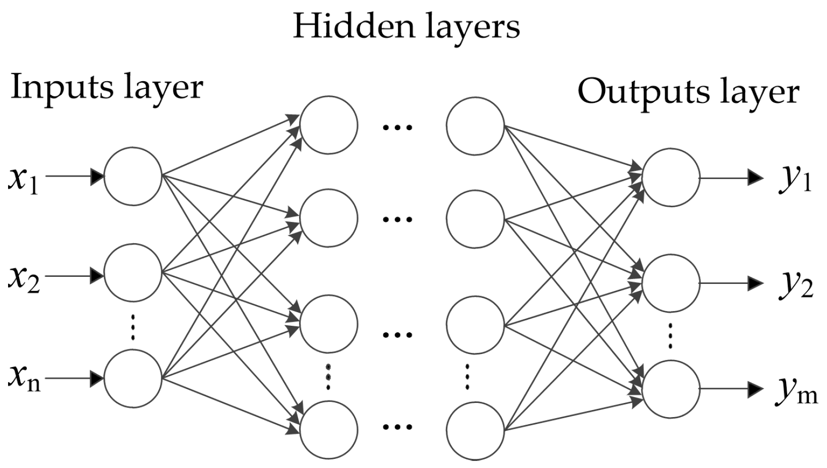
An artificial neural network (ANN) is a mathematical model and network system inspired by the biological neural network of the human brain. An ANN is made up of a collection of connected units called artificial neurons, which receive input, change their activation state according to the input, and produce output depending on the input and activation [32]. The weights and thresholds of the neurons can be modified by a process called learning. The backpropagation (BP) algorithm, a supervised gradient–descent learning algorithm, is a learning rule used most frequently in ANNs to calculate a gradient that is needed in the calculation of the weights. The BP network, which is trained through the BP algorithm, is the most widely used neural network at present. Structurally, the BP network is a kind of feedforward ANN consisting of three or more layers (an input layer, one or more hidden layers, and an output layer). Each node in a layer is connected to every node in the next layer with a certain weight. There exists no connection between nodes in the same layer. Except for input nodes, each node is a neuron that uses an activation function. The structure of the BP network is shown in Figure 3.

The basic idea of the BP algorithm is minimizing the mean squared error of the outputs by adjusting the connection weights after each learning iteration. The algorithm mainly include two processes: the forward propagation of the signal and backpropagation of the error. Regarding the forward propagation of the signal, the input sample is transmitted to the output layer by going from a layer to a next layer. If the actual output of the output layer does not match the expected output, the error propagation is shifted to the error backpropagation process. In the other case, the learning algorithm stops. During error backpropagation, the output error is propagated back to the input layer through the hidden layers. The error gradient is reduced to the allowable minimum by adjusting the connection weights and thresholds between the nodes of the former and of latter layer. Adjusting weights and thresholds is the network learning or training process.

The standard BP algorithms, such as gradient–descent and gradient–descent with momentum, are often too slow because of their inherent defects. In practice, successful training always depends on the appropriate learning rate and momentum constant [39]. To eliminate the disadvantages of BP learning algorithms, faster algorithms, e.g., resilient backpropagation, scaled conjugate gradient, and Levenberg–Marquardt, are included in the training of BP networks.

3. Condition Monitoring Approach for Shearing Machines

For monitoring the health state of the shearing machines exactly, a condition monitoring approach consistsing of WPT–based feature extraction and hybrid HMM–ANN based fault diagnosis model and detection steps were presented.

3.1. Feature Extraction Method Based on WPT

Feature extraction is applied to decrease the dimension of the original signal, keep and strengthen useful information, reduce or even eliminate interference information, and to highlight feature information by transforming the signal form. As is already known, noises of a shearing machine contain a lot of information on the health state. When the health state changes, the amplitude–frequency and phase–frequency characteristics in the frequency domain will change, and the energy in each frequency band will change to a different value. As mentioned above, WPT is suitable for analyzing nonlinear and non–stationary signals containing large amounts of details just like the noises of the shearing machine.

The energy in every frequency band can be calculated by the wavelet packet coefficients. Then, the health state of the shearing machine can be recognized by analyzing the energy distribution. By decomposing the signal, the wavelet packet coefficients of every frequency band can be obtained. Hence, the subband signals of $n^{th}$ level can be reconstructed with the wavelet packet coefficients. The energy of each band in the $n^{th}$ level can be expressed as the square sum of the corresponding node’s wavelet packet coefficients:

$$E_i=\sum _{k=1}^m{\left|c_{ik}\right|}^2,(i=0,1,\cdots ,2^n-1),$$

(6)

where $E_i$ is the energy of the reconstructed signal $s_{ni}$, $c_{ik}$ the wavelet packet coefficient of $s_{ni}$, and n the level of the wavelet packet decomposition. The total energy of the signal is calculated with:

$$E_T=\sum _{i=0}^{2^n-1}{E}_i.$$

(7)

Therefore, for a n–level WPT feature extraction, the energy feature vector is obtained by normalizing the energy of every frequency band in the $n^{th}$ layer:

$$T=\left[\frac{E_0}{E_T},\frac{E_1}{E_T},\cdots ,\frac{E_{2^n-1}}{E{}_T}\right].$$

(8)

3.2. Hybrid HMM–ANN Model for Fault Diagnosis

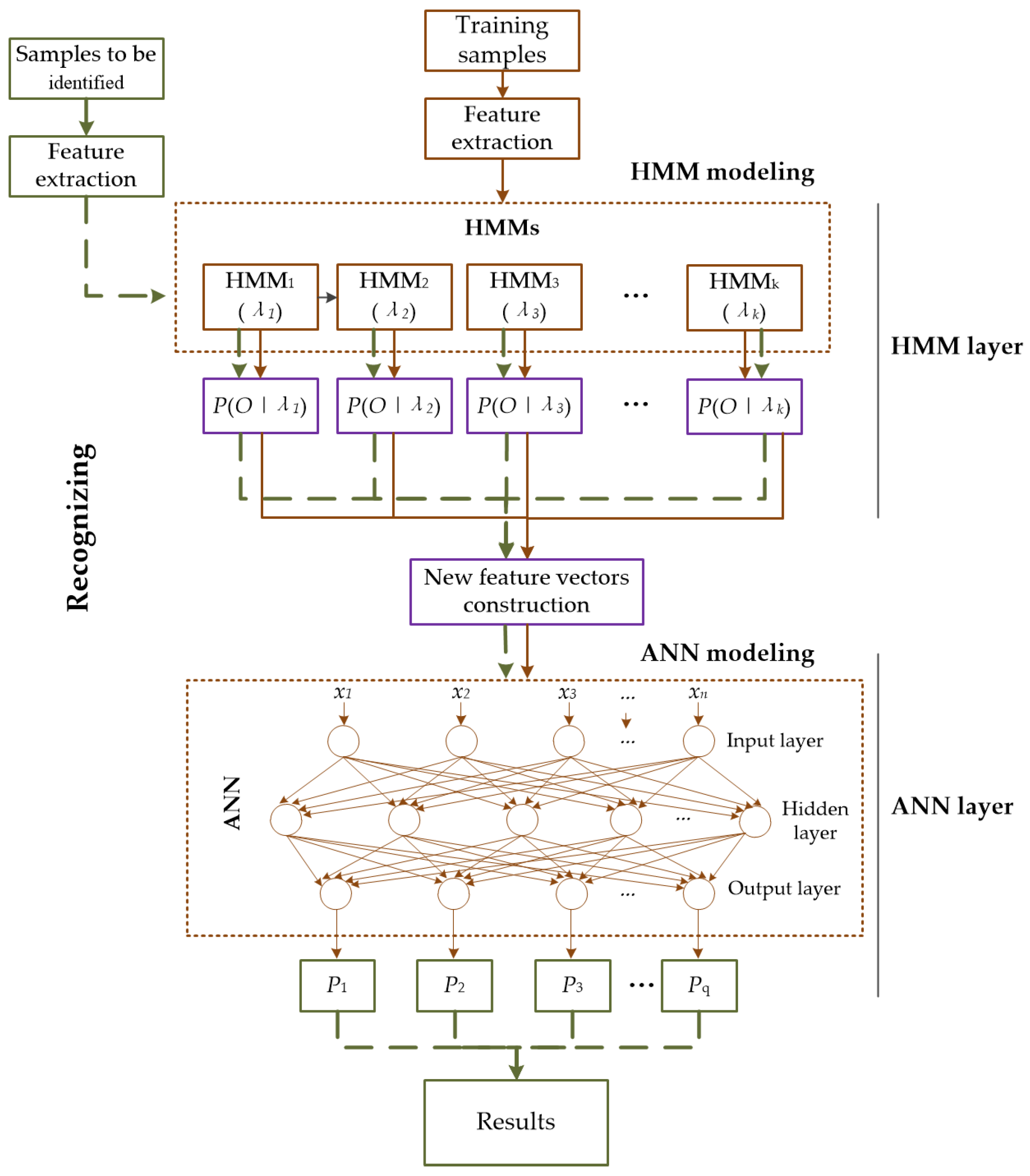
The HMM possesses a strong dynamic–modeling ability because it can be applied to analyze a time series of states. When using it for classification, the method gives the categorizing result according to the model producing the highest likelihood. If the signal to be recognized is contaminated by noise, the output probabilities of several HMMs may be very close and can lead to an incorrect recognition. As mentioned above, an ANN exhibits strong robustness, fault tolerance, learning ability, and self-adaptability. It is not sensitive to incomplete input information or characteristic defects. However, during recognition, the samples are classified according to the signal characteristics of the current time series, without considering the relation between “front and back time series”. Thus, the ANN model may lead to unrealistic results. In conclusion, the advantages of HMM and ANN are complementary. In this study, a hybrid HMM–ANN model was constructed by combining HMM’s dynamic–modeling ability and ANN’s high robustness, fault tolerance, learning ability, and self-adaptability. The hybrid model consists of two layers: the HMM layer and the ANN layer. The structure is shown in Figure 4.

The HMM layer is in the upper layer, thereby enabling the hybrid mode’s strong dynamic–modeling ability. The HMM layer consists of a modeling module and an output probability calculation module. The modeling module is used to obtain the HMMs by learning the samples, while the output probability calculation module is used to calculate the output probabilities of samples under each of the HMMs. The ANN layer is in the lower layer, taking the advantage of ANN’s fault tolerance, learning ability and self–adaptability. It contains an input layer, several hidden layers and an output layer. The hybrid HMM–ANN model is trained by the learning process and produces the predicted outputs.

3.3. Training and Recognizing Process of the Hybrid HMM–ANN Model

3.3.1. Training Process of the Hybrid Model

As is shown in Figure 4, the training of hybrid HMM–ANN model (HMM–ANN modeling) includes three processes: HMM training, ANN input/target vectors construction and ANN training.

(1) Selection and Training of HMM.

Compared with discrete HMM, the continuous HMM has low distortion and better classification effect [30]. Thus, a continuous Gaussian mixture hidden Markov model (CGHMM) was chosen. The probability density of each state is determined jointly by two Gaussian probability density functions. A CGHMM can be expressed as:

$$\lambda =(\pi ,A,{\mu }_{jk},{\sigma }_{jk},c_{jk}),$$

(9)

where ${\mu }_{jk}$ is the mean vector of the Gaussian function, ${\sigma }_{jk}$ the covariance matrix of the Gaussian mixture, $c_{jk}$ the mixing coefficient matrix, and the index j denotes the state of HMM, k the Gaussian mixture. The training procedure is as follows:

(a)

Initial guess of parameters. It is generally considered that the initial values of parameters $\pi$ and A have little effect while the initial value of parameters ${\mu }_{jk}$, ${\sigma }_{jk}$ and $c_{jk}$ have a large influence on the training result of HMMs. The initial values $\pi$ and A can be set randomly or evenly. It will be detailed in the empirical part. The initial parameters ${\mu }_{jk}^{\left(0\right)}$, ${\sigma }_{jk}^{\left(0\right)}$ and $c_{jk}^{\left(0\right)}$ are estimated by using the segmental k–means algorithm (see literature [40]).

(b)

Model revaluation. In this study, the Baum–Welch algorithm was used to reevaluate the HMM parameters. For each state of HMM, the constructed model $\lambda$ is updated based on the following revaluation equations:

$$\begin{array}{l}{\widehat{\pi }}_i={\gamma }_1\left(i\right),\\ {\widehat{a}}_{ij}=\sum _{t=1}^{T-1}{\xi }_t(i,j)/\sum _{t=1}^{T-1}{\gamma }_t\left(i\right),\\ {\widehat{c}}_{jk}=\sum _{t=1}^T{\gamma }_t(j,k)/\sum _{t=1}^T\sum _{k=1}^M{\gamma }_t(j,k),\\ {\widehat{\mu }}_{jk}=\sum _{t=1}^T{\gamma }_t(j,k)·o_t/\sum _{t=1}^T{\gamma }_t(j,k),\\ {\widehat{\sigma }}_{jk}=\sum _{t=1}^T{\gamma }_t(j,k)·{(o_t-{\mu }_{jk})}^2/\sum _{t=1}^T{\gamma }_t(j,k),\end{array}$$

(10)

where ${\gamma }_t\left(i\right)=P\left(q_t={\theta }_i\right|O,\lambda )$ is the probability of being in state ${\theta }_i$ at time t given the observed sequence O and model $\lambda$, ${\xi }_t(i,j)=P(q_t={\theta }_i,q_{t+1}={\theta }_j|O,\lambda )$ the probability of being in state ${\theta }_i$ and ${\theta }_j$ at times t and $t+1$ respectively given the observed sequence O and model $\lambda$.

(c)

Model determination. The output probabilities of the samples under the new model $P\left(O\right|\lambda )$ are calculated by using the forward–backward algorithm. If the condition $P\left(O\right|{\lambda }^{(n+1)})-P\left(O\right|{\lambda }^{\left(n\right)})\le \epsilon$ is met, the model obtained in the last revaluation is considered the final model. Otherwise, return to step (b) and continue reevaluating.

(2) Construction of Input/Target Vectors of ANN.

The feature vectors of the training samples are fed to the HMM layer to calculate the output probabilities of the samples for every HMM. The input vectors of ANN can be constructed with the normalized probabilities of the samples under each of the trained HMMs. The target vectors are constructed according to the state of the samples. The target probability is 1 if the sample belongs to this health state and 0 if not.

(3) Selection and Training of ANN.

The selection and training procedure of ANN mainly includes the construction of training samples, the selection of the ANN network model, and the training of ANN:

(a)

Establishment of network. An ANN with three layers (input layer, output layer, and hidden layer) is constructed. The number of neurons in the input layer is equal to the dimension of the feature vector, and that of the output layer equals the number of health states. The number of neurons in the hidden layer is mainly determined by tests, while the following empirical equation gives a preliminary range:

$$h=\sqrt{(m+n)}+a$$

(11)

where m is the number of neurons in the input layer, n the number of neurons in the output layer, and a an integer constant between 1 and 10. Besides the network structures, the activation functions are critical points for the performance of ANNs.

(b)

Setting training parameters, e.g., selections of initial weight, threshold, goal, learning rate, momentum factor, maximum epochs, as well as selections of learning function, training function, and performance function. They are also selected according to their applicabilities, requirements of tasks and through tests.

(c)

Training of ANN. Use the samples to train ANN iteratively until the accuracy meets the goal value or the accuracy does no longer improve. Thus, the trained ANN model is obtained.

3.3.2. Recognizing Process of the Hybrid Model

The recognizing process of the hybrid HMM–ANN model is as follows:

(a)

Construction of input vectors for ANN. The samples to be identified are preprocessed and feature extracted with the same method as used for training samples. Consequently, observed vectors can be obtained. Next, use the feature vectors as input to calculate the output probabilities of the samples to be identified for all trained HMMs. The input vectors of ANN are constructed with these probability values.

(b)

Probability prediction of samples to be identified for each health state. Using the input vectors to produce the outputs of the trained ANN model. As a result, the predicted probabilities of the samples to be identified for each health state are obtained.

(c)

Classification decision. Finally, considering the highest likehood, the health states of the samples to be identified are determined.

4. Application and Results

In order to check the performance of the proposed approach, a shearing experiment was carried out in lab environments, and the approach was validated using the noise signals that were acquired in the experiment.

4.1. Experimental Rig Setup and Data Collection

4.1.1. Experimental Setup

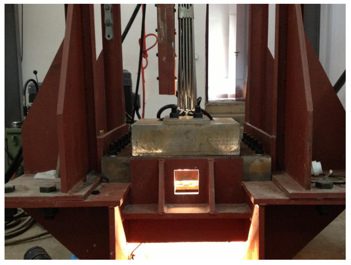
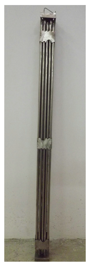
The shearing experiment was carried out on a simulated spent fuel shearing machine that can simulate the working processes (e.g., gripping, feeding and shearing of fuel assemblies) of the real shearing machines. The simulated fuel assembly was designed according to the structure of AFA–2G fuel assembly, and was simplified and reduced in scale. The structure of the fuel rods were made of 304 stainless steel, and the fuel rods were filled with Al${}_2$O${}_3$ ceramic blocks instead of UO${}_2$. The simulated shearing machine and fuel assembly are shown in Figure 5 and Figure 6. The main parameter settings of the simulated shearing experiment are shown in the

Table 1. The main parameter settings of the simulated shearing experiment.

Maximum Pressing Force	Maximum Shearing Force	Tool Feeding Speed	Feeding Step Distance	Section Size
165 kN	785 kN	0.03 m/s	15 mm	65 × 65 mm

. In addition, an InLine 1000 high–speed camera (made by Fastec Imaging Corporation, San Diego, CA, USA) was used to record the shearing process through an observation hole designed on the simulated shearing machine.

4.1.2. Noise Acquisition Method for Shearing Machines

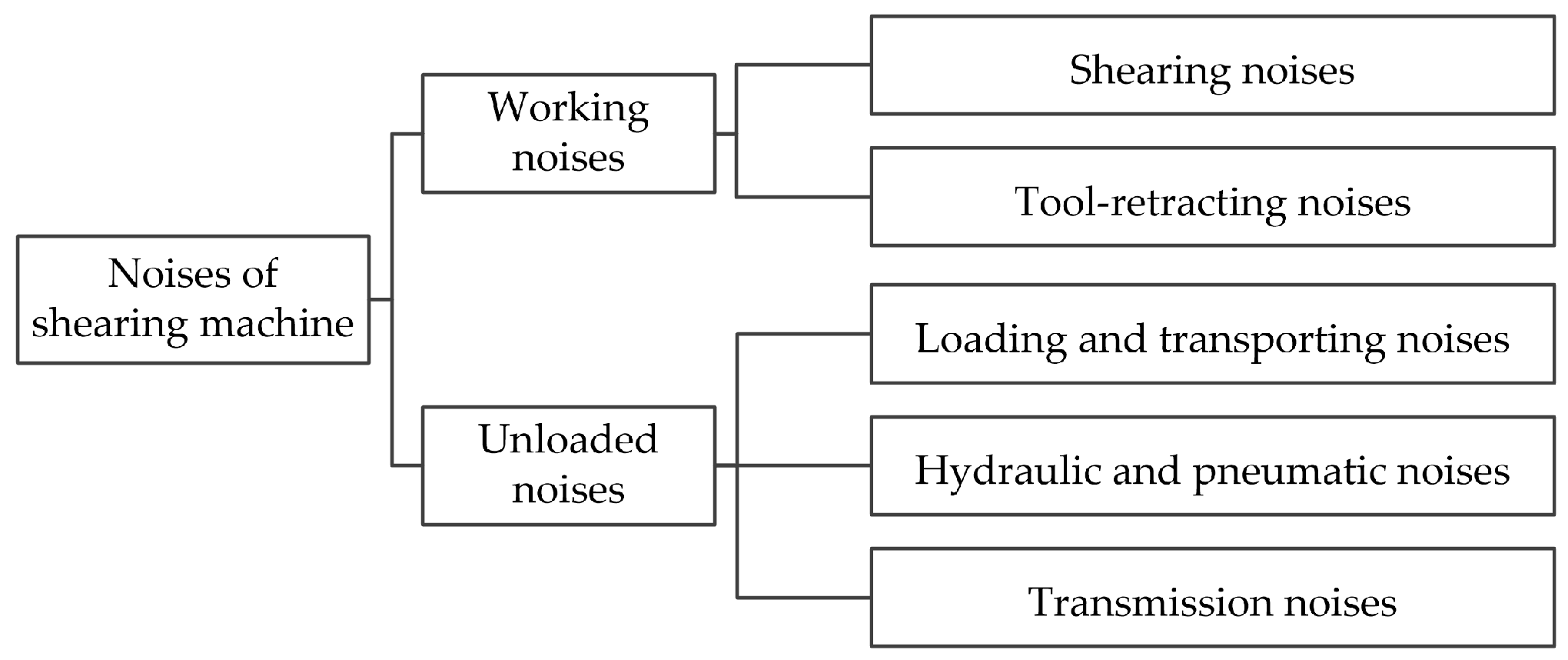
The shearing machine, a complex piece of mechanical equipment, possesses many sound sources. The noises of a shearing machine can be divided into working noises and unloaded noises. The working noises mainly include shearing noises and tool–retracting noises. The unloaded noises are generated by the shearing machines during unloaded operation, e.g., noises generated by the hydraulic and pneumatic system, noises generated during loading and transport of material, and noises caused by clearance of transmission components such as gears, push chains, bearings, and tool carriers. The composition of shearing–machine noises is shown in Figure 7.

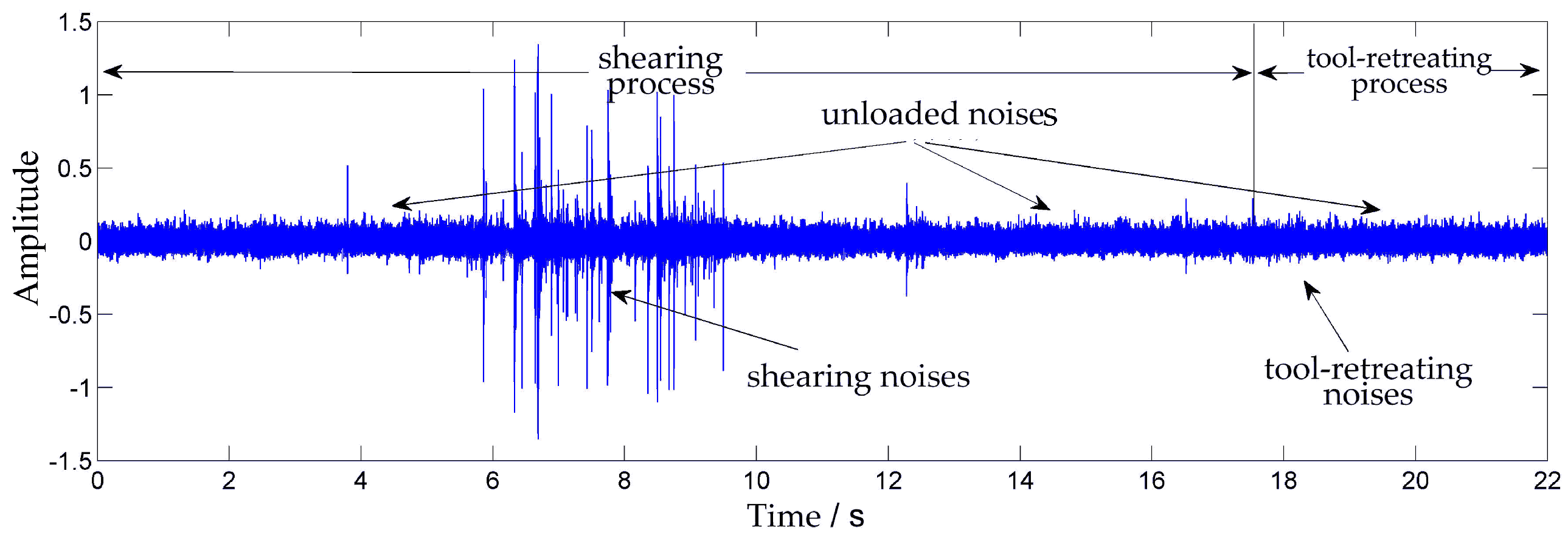
The acquisition period equalled a complete working cycle of the shearing machine including feeding process, shearing process, and tool–retreating process. Figure 8 shows a diachronic sound pressure curve of the working cycle of a shearing machine. The curve clearly indicates the unloaded noise, shearing noises, and tool–retreating noises. It is obvious that the shearing noises are most intense.

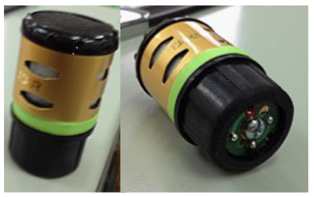
The moving–coil microphone has excellent anti–irradiation properties because it has no electronic components or integrated circuits inside. Furthermore, benefitting from the high peak voltage of its output signal, the ionizing noises caused by radiation have no significant effect on the signals. Experiments showed that the moving-coil microphone can work without significant distortion after receiving a total dose of 5.7 kGy [41]. In this study, the TS–5 moving–coil microphones (made by Guangdong Takstar Electronic Co., Ltd., Huizhou, Guangdong, China) were chosen as the components of the noise-acquisition unit, as shown in Figure 9.

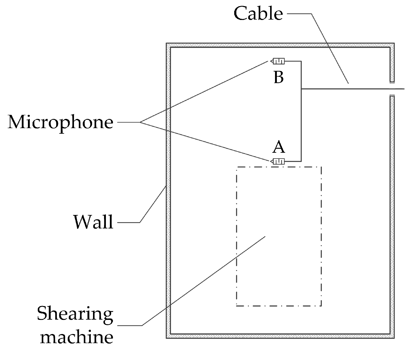
To reduce the influence of background noises and operation noises, the noise–acquisition unit was designed as a dual microphone. Microphone A was positioned near the shearing machine while microphone B was positioned far away, as shown in Figure 10. As the distributions of background noises are uniform, the difference of the background noises picked up by the two microphones is not significant, while the energy and pressure of the working noises produced by shearing machines decrease fast with the increasing distance from the sound sources. Therefore, the working noises picked up by microphone A are much stronger than that of microphone B. Thus, using the difference between the two sound channels, the signals are denoised.

After the denoising, the PCI–6280 data acquisition card (made by National Instruments Corporation, Austin, TX, USA) was used for digital sampling of the signals. The spectrum analysis of the noise signals showed that the energy is mainly within 7 kHz, and the maximum frequency does not lie above 20 kHz. According to the Nyquist theorem, the sampling rate is at least two times higher than the highest frequency of the analyzed signals. Hence, the sampling rate was set to 44.1 kHz. The sampled data are saved as “.wav” audio files.

4.1.3. Collected Data

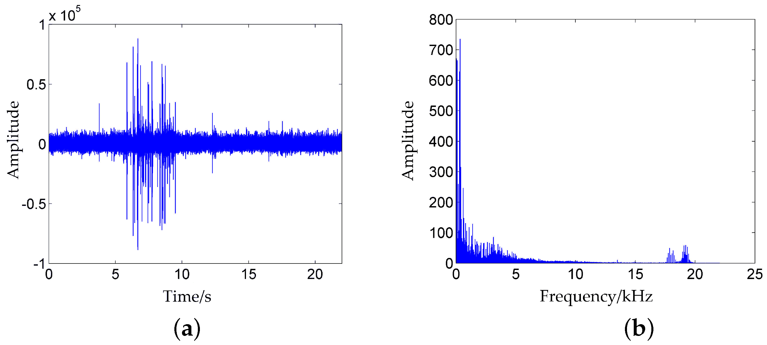
After each shearing, the tool wear condition and the opening rates of the fuel–rod segments were checked to confirm the health state of the shearing machine. For the subsequent signal processing using Matlab (R2015a, MathWorks Inc., Natick, MA, USA), the “.wav” audio files were converted to the “.mat” data files. For an example, the time domain and frequency domain diagrams of noise sample No. 1–32 are shown in Figure 11.

In this experiment, 170 valid samples were collected. The settings of health states and sample indices are listed in

Table 2. Settings of health states and sample indices.

State No.	States	Sample Indices
1	Normal (Normal state without faults)	1–1 to 1–45
2	Fault 2 (Slight tool wear)	2–1 to 2–40
3	Fault 3 (Severe tool wear)	3–1 to 3–50
4	Fault 4 (Damaged tool)	4–1 to 4–35

.

4.2. Results and Discussions

4.2.1. Feature Extraction from Noise Samples

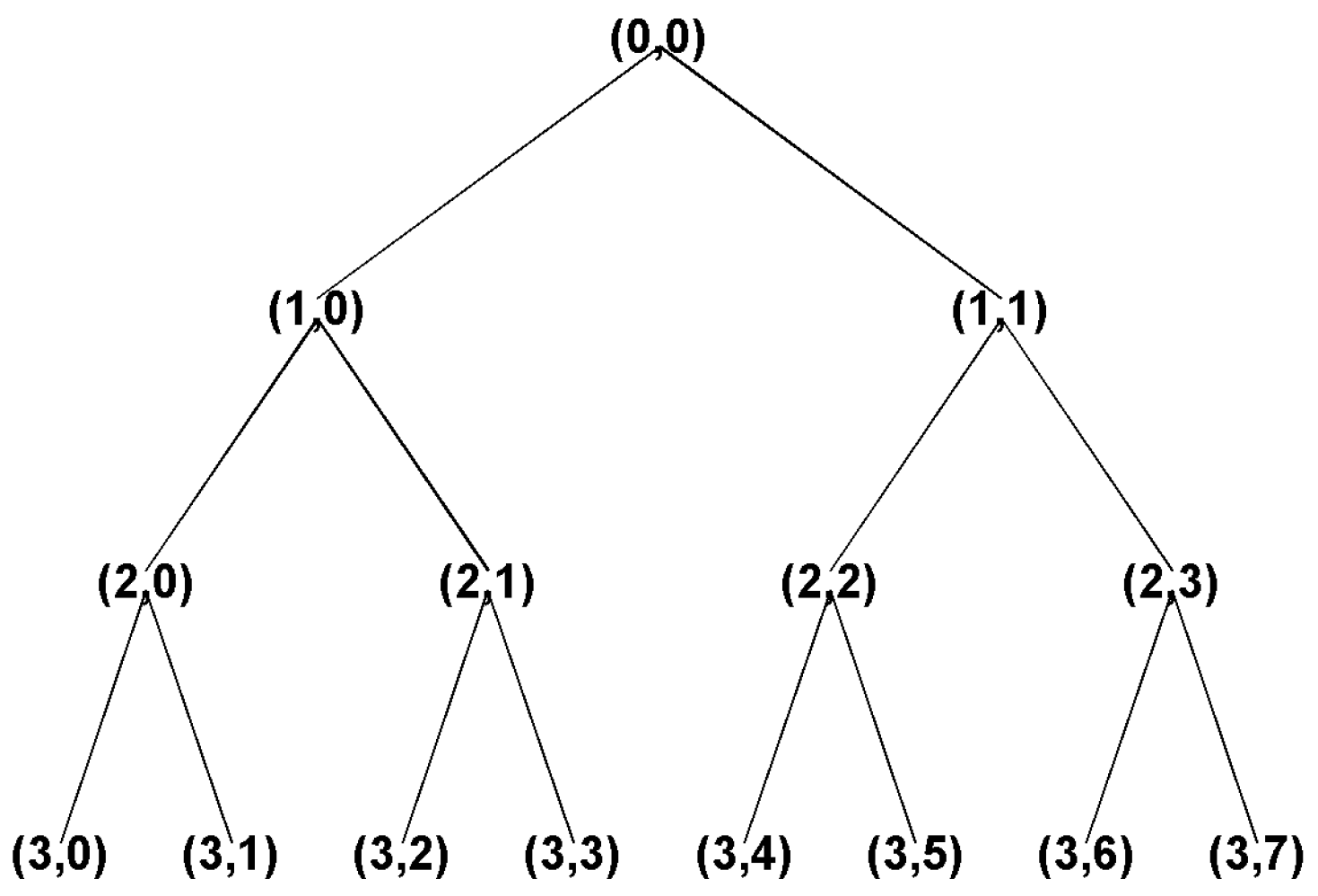
When using WPT for feature extraction, the decomposition level n is particularly critical because the recognition accuracy rate is directly related to n. If n is too small, the energy is mainly concentrated in some certain subbands, resulting in very little difference in the feature distribution of different signals. The signals can not be distinguished effectively by the extracted features, while, if n is too large, it will cause “dimension disaster”, which is the feature redundancy and empty subbands, and increases the complexity of the classifier, eventually reducing the recognition accuracy rate. In the test, when n was less than or equal to two, the recognition rate was less than 70%, while, when n was greater than or equal to four, some empty bands appeared. It is appropriate to set n to be three, where the energy features’ dimension is eight. Furthermore, from tests, the db5 wavelet function and Shannon entropy were selected for a three–level wavelet packet decomposition of the noise signals. The wavelet packet decomposition tree is shown in Figure 12.

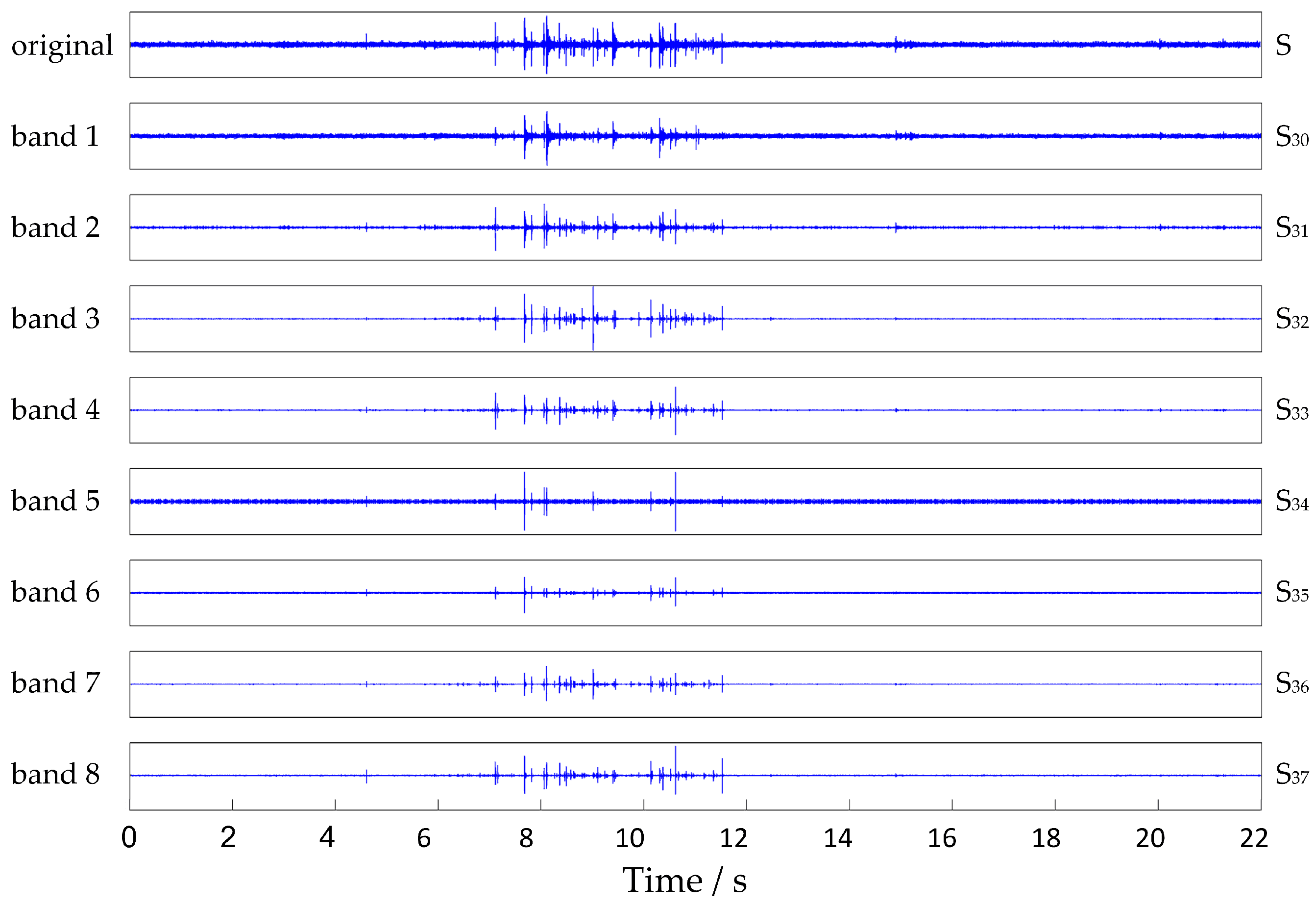
To provide an example, the subband signals, which were reconstructed by the third–level nodes of the noise sample No. 1–32, are shown in Figure 13. It indicates that eight subbands were decomposed from the original signal.

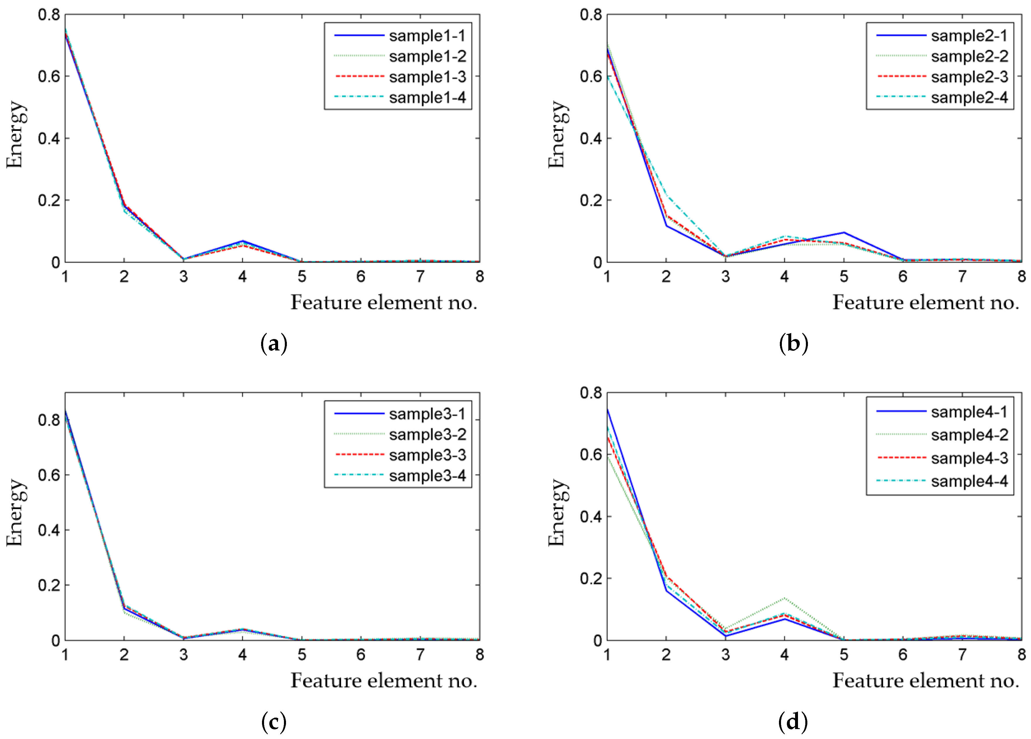
The feature vectors of the first four samples of each health state are provided as examples in Figure 14a–d.

The mean of feature element values in every frequency band of all samples for every health state are listed in

Table 3. Mean of feature element values of all samples in every frequency band for every health state.

Working State No.	Mean of Feature Element Values of All Samples in Every Frequency Band
	band 1	band 2	band 3	band 4	band 5	band 6	band 7	band 8
1	0.7358	0.1819	0.0107	0.0622	0.0007	0.0021	0.0043	0.0023
2	0.6748	0.1537	0.0196	0.0779	0.0544	0.0054	0.0095	0.0046
3	0.7828	0.1283	0.0161	0.0506	0.0034	0.0041	0.0088	0.0060
4	0.6697	0.2064	0.0199	0.086	0.001	0.0027	0.0094	0.0049

, and the comparison of the average energies of each frequency band for different health states is shown in Figure 15a–h.

It can be seen in Figure 15 that the average energy of every frequency band for different health states are significantly different. Therefore, the feature extraction method based on WPT is effective for noise signals of shearing machines.

4.2.2. HMM–ANN Modeling and Fault Detection Results

In this study, 60% of the samples in each state were randomly chosen as training sets, while the remaining 40% were put aside for testing. The numbers of samples of each sample sets and state category are shown in

Table 4. The numbers of samples of each sample sets and state category.

Sample Sets	Normal	Fault 2	Fault 3	Fault 4	Total
Training	27	24	30	21	102
Testing	18	16	20	14	68

.

The tool wear process is continuous and irreversible, that is, the latter state can not transition back to the previous state. Therefore, the left–right HMM (which permit only left to right transitions) with good effect and fast speed was chosen. The number of states was set to be N = 4. Since the initial state was “normal”, the initial state distribution was set to be ${\pi }^{\left(0\right)}=[1,0,0,0]$. In addition, the initial state–transition probability matrix was set evenly to be

$$A^{\left(0\right)}=\left[\begin{array}{cccc}\hfill 0.5& \hfill 0.5& \hfill 0& \hfill 0\\ \hfill 0& \hfill 0.5& \hfill 0.5& \hfill 0\\ \hfill 0& \hfill 0& \hfill 0.5& \hfill 0.5\\ \hfill 0& \hfill 0& \hfill 0& \hfill 1\end{array}\right].$$

The initial shape of the chosen HMM are shown in Figure 16.

In accordance with the general practice, purelin (linear activation function) was used for the output layer of ANN. Logsig (sigmoid function) is very similar to tansig (hyperbolic tangent function function) [42]. However, tansig is considered to be better for its range is normalized from −1 to 1 while logsig is vertically translated to normalize from 0 to 1. Thus, tansig was chosen as the activation function of the hidden layer. According to the activation function, the initial weights should be randomly selected between (−1, 1). In this study, the initial weights and thresholds were randomly generated by the newff function in Matlab’s neural network toolbox. The learning rate was set to 0.01, the momentum factor to 0.9, and the maximum epochs to 300. The learning function chose learngdm (gradient descent with momentum weight and bias learning function), and the performance function chose mse (mean squared error performance function). For eliminating some disadvantages of the gradient–descent method, such as the slow training speed, the traingdx (gradient descent with adaptive learning rate), trainrp (resilient backpropagation), trainlm (Levenberg–Marquardt), and trainscg (scaled conjugate gradient) algorithms were selected as candidate algorithms for network training. To select the optimal parameter setting of ANN, more than twenty various parameter settings were tested, partly shown in

Table 5. The performance of ANN for different settings.

Training Rule	Neurons in Hidden Layer	Training Error (mse)	R
trainlm	10	3.10 $\times {10}^{-10}$	1
traingdx	10	5.00 $\times {10}^{-2}$	0.85633
trainrp	10	4.62 $\times {10}^{-2}$	0.86827
trainscg	10	1.44 $\times {10}^{-2}$	0.96095
trainlm	5	2.26 $\times {10}^{-3}$	0.99397
trainlm	8	3.40 $\times {10}^{-5}$	0.99991
trainlm	12	7.12 $\times {10}^{-9}$	1
trainlm	14	2.22 $\times {10}^{-8}$	1

. The table indicates that a network with ten neurons in the hidden layer proves to be an optimal ANN, and the trainlm (Levenberg–Marquardt) proves to be the best training function.

The extracted energy feature vectors of the training samples (known state categories) were fed to the HMM layer. Then, some HMMs were obtained by learning the samples. The goal for the ANN training was set to ${10}^{-4}$. The input/target vector pairs (constructed by the method mentioned above) were fed to the ANN layer. After the training converged, the ANN model was obtained.

The extracted energy feature vectors of the testing samples were fed to the trained hybrid HMM–ANN model. The predicted values are shown in

Table 6. Comparisons of health states and HMM–ANN outputs.

States	State No.	Predicted Values
Normal	1	1	3	3	1	1	1	1	1	1	1	1	1	1	1	1	1	1	1	–	–
Fault 2	2	2	3	2	2	2	3	2	2	2	2	2	2	2	2	2	2	–	–	–	–
Fault 3	3	3	3	3	3	3	3	3	3	3	3	3	3	3	4	3	3	3	4	3	3
Fault 4	4	4	4	4	4	4	4	4	4	4	4	4	4	4	4	–	–	–	–	–	–

Total samples for validation: 68, correct predictions: 62, accuracy rate: 91.18%.

.

As seen in Table 6, 68 samples including normal and faulty health states were used in the prediction, and 91.18% samples (a total of 62) were predicted correctly. Especially for the samples of fault 4 (damaged tool), the accuracy rate reached 100%.

4.2.3. Comparative Analysis Results

To verify the enhancement of the HMM–ANN prediction accuracy, two more comparison experiments were carried out. An isolated HMM model and an isolated ANN model were established. For comparison purposes, the isolated HMM and ANN model used the same parameter settings and initial values (or initialization method) as for the hybrid HMM–ANN model. Furthermore, the same training and testing sample sets were applied, and the same three–level WPT method was used for feature extraction. The extracted energy feature vectors of the training samples (known state categories) were fed to train the isolated HMM. In addition, the input/target vector pairs (the input vectors were the extracted energy feature vectors, target vectors were constructed by the above mentioned method) are fed to train the isolated ANN. Then, the feature vectors of the testing samples were fed to the trained HMM and ANN. The results are shown in

Table 7. Comparison of health states and HMM outputs.

States	State No.	Predicted Values
Normal	1	1	1	3	2	1	1	1	1	1	2	1	1	1	1	1	1	1	1	–	–
Fault 2	2	2	4	2	2	2	4	2	2	2	2	2	2	2	2	2	2	–	–	–	–
Fault 3	3	3	3	3	3	3	3	3	2	3	3	2	3	2	3	3	3	3	2	3	3
Fault 4	4	4	4	4	4	4	4	4	4	4	4	4	4	4	4	–	–	–	–	–	–

Total samples for validation: 68, correct predictions: 59, accuracy rate: 86.76%.

and

Table 8. Comparisons of health states and ANN outputs.

States	State No.	Predicted Values
Normal	1	4	3	3	4	4	4	1	1	1	4	1	1	1	1	1	1	1	1	–	–
Fault 2	2	4	2	2	2	2	2	4	4	2	2	2	2	2	2	4	2	–	–	–	–
Fault 3	3	3	3	3	4	3	3	4	4	4	3	2	3	4	4	3	3	3	3	4	3
Fault 4	4	2	4	4	2	1	4	2	4	2	4	4	2	2	4	–	–	–	–	–	–

Total samples for validation: 68, correct predictions: 42, accuracy rate: 61.76%.

.

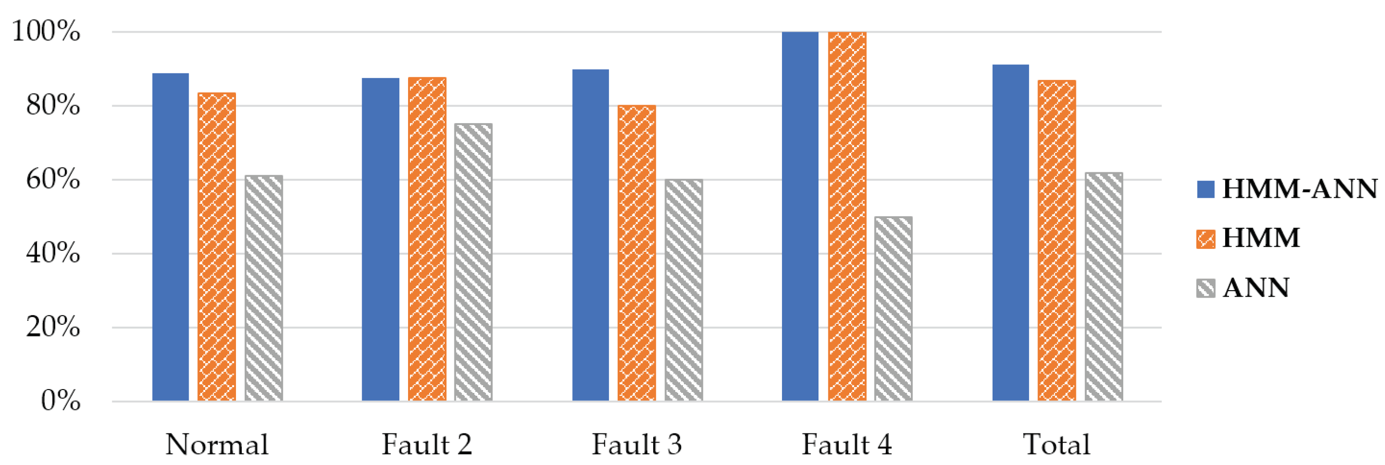
Comparing Table 6 with Table 7 and Table 8 shows that some prediction errors in the isolated HMM or ANN model were correctly predicted in the hybrid HMM–ANN model. As seen from Figure 17, for Faults 1 and 3, the hybrid model gave better results than the isolated HMM, while, for Faults 2 and 4, they had the same accuracy rates. By contrast, for each health state, the hybrid model gave better results than the isolated ANN model. Furthermore, the total accuracy of the hybrid HMM–ANN model was significantly higher than that of the isolated HMM or ANN model.

Note that accuracy of the proposed approach strictly depends on the availability of the complete (e.g., in each health state) condition monitoring data. Hence, to avoid accuracy reduction in fault diagnostics, the proposed approach should be validated with the complete data samples.

5. Conclusions

In this paper, an intelligent condition monitoring approach consisting of WPT–based feature extraction and hybrid HMM–ANN based fault detection steps was proposed. The proposed approach was validated using the noise signals, which were acquired from shearing machines under the lab environments. The verification results showed that the extracted features of the working noises can well characterize the health states of shearing machine, the hybrid model which combined the advantage on dynamic–modeling of HMM and pattern recognition of ANN is effective—the accuracy rate is significantly higher than that of the isolated HMM or ANN model.

References

1. Poinssot, C.; Bourg, S.; Ouvrier, N.; Combernoux, N.; Rostaing, C.; Vargas-Gonzalez, M.; Bruno, J. Assessment of the environmental footprint of nuclear energy systems. Comparison between closed and open fuel cycles. Energy 2014, 69, 199–211. [Google Scholar] [CrossRef]
2. Nash, K.L.; Nilsson, M. 1—Introduction to the reprocessing and recycling of spent nuclear fuels. In Reprocessing and Recycling of Spent Nuclear Fuel; Taylor, R., Ed.; Woodhead Publishing: Oxford, UK, 2015. [Google Scholar]
3. Silverio, L.B.; de Queiroz Lamas, W. An analysis of development and research on spent nuclear fuel reprocessing. Energy Policy 2011, 39, 281–289. [Google Scholar] [CrossRef]
4. Hanson, B. 6—Process engineering and design for spent nuclear fuel reprocessing and recycling plants. In Reprocessing and Recycling of Spent Nuclear Fuel; Taylor, R., Ed.; Woodhead Publishing: Oxford, UK, 2015. [Google Scholar]
5. Zou, S.L.; Xie, Y.P.; Wang, K.; Tang, D.W. Reliability analysis and experimental research on cutting tool of vertical shearing machine. Adv. Mater. Res. 2014, 889–890, 441–449. [Google Scholar] [CrossRef]
6. Zhang, X.Z.; Zhao, L.H.; Deng, Q.; Song, C. Application of wavelet packet analysis in fault diagnosis of spent nuclear fuel shears. J. Univ. South China (Sci. Technol.) 2014, 28, 69–73. [Google Scholar]
7. Wang, Y.S.; Ma, Q.H.; Zhu, Q.; Liu, X.T.; Zhao, L.H. An intelligent approach for engine fault diagnosis based on hilbert–huang transform and support vector machine. Appl. Acoust. 2014, 75, 1–9. [Google Scholar] [CrossRef]
8. Tafreshi, R. Feature Extraction Using Wavelet Analysis with Application to Machine Fault Diagnosis. Ph.D. Thesis, University of British Columbia, Vancouver, BC, Canada, 2005. [Google Scholar]
9. Lenka, B. Time–frequency analysis of non–stationary electrocardiogram signals using Hilbert-Huang Transform. In Proceedings of the IEEE International Conference on Communications and Signal Processing, Melmaruvathur, India, 2–4 April 2015; pp. 1156–1159. [Google Scholar]
10. Yang, Y.; Zhang, W.; Peng, Z.; Meng, G. Time–frequency fusion based on polynomial chirplet transform for non–stationary signals. IEEE Trans. Ind. Electron. 2012, 60, 3948–3956. [Google Scholar] [CrossRef]
11. Sun, M.; Cui, S.; Xu, Y. Design and implementation of a time–frequency analysis system for non-stationary vibration signals using mixed programming. Int. J. Hybrid Inf. Technol. 2014, 7, 283–294. [Google Scholar] [CrossRef]
12. Burriel-Valencia, J.; Puche-Panadero, R.; Martinez-Roman, J.; Sapena-Bano, A.; Pineda-Sanchez, M. Short-frequency fourier transform for fault diagnosis of induction machines working in transient regime. IEEE Trans. Instrum. Meas. 2017, 66, 432–440. [Google Scholar] [CrossRef]
13. Climente-Alarcon, V.; Antonino-Daviu, J.A.; Riera-Guasp, M.; Vlcek, M. Induction motor diagnosis by advanced notch fir filters and the wigner–ville distribution. IEEE Trans. Ind. Electron. 2014, 61, 4217–4227. [Google Scholar] [CrossRef]
14. Torrence, C.; Compo, G.P. A practical guide to wavelet analysis. Bull. Am. Meteorol. Soc. 1998, 79, 61–78. [Google Scholar] [CrossRef]
15. Ren, H.; Ren, A.; Li, Z. A new strategy for the suppression of cross-terms in pseudo wigner–ville distribution. Signal Image Video Process. 2016, 10, 139–144. [Google Scholar] [CrossRef]
16. Daubechies, I. The wavelet transform, time-frequency localisation and signal analysis. J. Renew. Sustain. Energy 2015, 36, 961–1005. [Google Scholar]
17. Fei, S.W. Fault diagnosis of bearing based on wavelet packet transform–phase space reconstruction–singular value decomposition and svm classifier. Arab. J. Sci. Eng. 2017, 42, 1967–1975. [Google Scholar] [CrossRef]
18. Su, J.; Chen, W.H. Model–based fault diagnosis system verification using reachability analysis. IEEE Trans. Syst. Man Cybern. Syst. 2017, 1–10. [Google Scholar] [CrossRef]
19. Li, Y.H.; Wang, J.Q.; Wang, X.J.; Zhao, Y.L.; Lu, X.H.; Liu, D.L. Community detection based on differential evolution using social spider optimization. Symmetry 2017, 9, 183. [Google Scholar] [CrossRef]
20. Ding, S.X. Model–Based Fault Diagnosis Techniques: Design Schemes, Algorithms, and Tools; Springer: London, UK, 2013. [Google Scholar]
21. Atamuradov, V.; Medjaher, K.; Dersin, P.; Lamoureux, B.; Zerhouni, N. Prognostics and health management for maintenance practitioners-Review, implementation and tools evaluation. Int. J. Progn. Health Manag. 2017, 8, 1–31. [Google Scholar]
22. Lang, L.I.; Liu, H.; Zhao, H. Review of vibration monitoring and fault diagnosis methods of wind turbines. Power Syst. Clean Energy 2017, 33, 94–100, 108. [Google Scholar]
23. Ramos, A.R.; Lázaro, J.M.B.D.; Prieto-Moreno, A.; Neto, A.J.D.S.; Llanes-Santiago, O. An approach to robust fault diagnosis in mechanical systems using computational intelligence. J. Intell. Manuf. 2017, 1–15. [Google Scholar] [CrossRef]
24. Witczak, M.; Pazera, M. Integrated fault diagnosis and fault–tolerant for constrained dynamic systems. In Proceedings of the International Conference on Diagnostics of Processes and Systems, Sandomierz, Poland, 11–13 September 2017; pp. 17–32. [Google Scholar]
25. Yang, B.; Yin, L.; Li, G.; Deng, W.; Zhao, H. Research on a new fault diagnosis method based on WT, improved PSO and SVM for motor. Recent Patents Mech. Eng. 2017, 9, 289–298. [Google Scholar]
26. Nose, T.; Kobayashi, T. A Study on Phone Duration Modeling Using Dynamic Features for Hmm–Based Speech Synthesis; Ieice Technical Report Natural Language Understanding and Models of Communication; IEICE: Tokyo, Japan, 2011; Volume 111, pp. 197–202. [Google Scholar]
27. Liao, Z.; Gao, D.; Lu, Y.; Lv, Z. Multi–scale hybrid HMM for tool wear condition monitoring. Int. J. Adv. Manuf. Technol. 2016, 84, 2437–2448. [Google Scholar] [CrossRef]
28. Tao, X.M.; Du, B.X.; Xu, Y. Bearings fault diagnosis based on HMM and fractal dimensions spectrum. In Proceedings of the IEEE International Conference on Mechatronics and Automation, Harbin, China, 5–8 August 2007; pp. 1671–1676. [Google Scholar]
29. Ntalampiras, S. Fault Identification in Distributed Sensor Networks Based on Universal Probabilistic Modeling. IEEE Trans. Neural Netw. Learn. Syst. 2015, 26, 1939–1949. [Google Scholar] [CrossRef] [PubMed]
30. Liu, X.; Liu, G.; Qiu, J. Hybrid HMM and SVM approach for fault diagnosis. Chin. J. Sci. Instrum. 2006, 27, 45–48, 53. [Google Scholar]
31. Mrugalski, M.; Luzar, M.; Pazera, M.; Witczak, M.; Aubrun, C. Neural network–based robust actuator fault diagnosis for a non-linear multi-tank system. ISA Trans. 2016, 61, 318–328. [Google Scholar] [CrossRef] [PubMed]
32. Venkat, V.; Chan, K. A neural network methodology for process fault diagnosis. AIChE J. 2010, 35, 1993–2002. [Google Scholar]
33. Patil, A.B.; Gaikwad, J.A.; Kulkarni, J.V. Bearing fault diagnosis using discrete wavelet transform and artificial neural network. In Proceedings of the IEEE International Conference on Applied and Theoretical Computing and Communication Technology, Bengaluru, Karnataka, India, 21–23 July 2016; pp. 399–405. [Google Scholar]
34. Tian, D.; Fan, L. A brain MR images segmentation method based on SOM neural network. In Proceedings of the IEEE International Conference on Bioinformatics and Bioengineering, Wuhan, China, 6–8 July 2007; pp. 686–689. [Google Scholar]
35. Bashir, Z.A.; El-Hawary, M.E. Applying wavelets to short–term load forecasting using PSO-based neural networks. IEEE Trans. Power Syst. 2009, 24, 20–27. [Google Scholar] [CrossRef]
36. Mao, X.; Chen, L.; Fu, L. Multi–level speech emotion recognition based on HMM and ANN. In Proceedings of the IEEE WRI World Congress on Computer Science and Information Engineering, Los Angeles, CA, USA, 31 March–2 April 2009; pp. 225–229. [Google Scholar]
37. Fan, X.; Zuo, M.J. Gearbox fault detection using hilbert and wavelet packet transform. Mech. Syst. Signal Process. 2006, 20, 966–982. [Google Scholar] [CrossRef]
38. Li, Z.; Liu, B.; Hou, J. Research on rotating machinery fault diagnosis method based on infinite hidden markov model. Chin. J. Sci. Instrum. 2016, 37, 2185–2192. [Google Scholar]
39. Ghobadian, B.; Rahimi, H.; Nikbakht, A.M.; Najafi, G.; Yusaf, T.F. Diesel engine performance and exhaust emission analysis using waste cooking biodiesel fuel with an artificial neural network. Renew. Energy 2009, 34, 976–982. [Google Scholar] [CrossRef] [Green Version]
40. Bhowmik, T.K.; Parui, S.K.; Kar, M. Segmental k-means algorithm based hidden Markov model for shape recognition and its applications. In Proceedings of the Sixth International Conference on Advances in Pattern Recognition, Kolkata, India, 2–4 January 2007; pp. 361–365. [Google Scholar]
41. Deng, Q. Irradiation experiments research of sound sensors. J. Univ. South China 2014, 28, 61–66. [Google Scholar]
42. Witczak, M. Toward the training of feed–forward neural networks with the D-optimum input sequence. IEEE Trans. Neural Netw. 2006, 17, 357–373. [Google Scholar] [CrossRef] [PubMed]
Figure 1. Map of wavelet packet decomposition.
Applsci 08 00838 g001
Figure 2. Composition of hidden Markov model.
Applsci 08 00838 g002
Figure 3. Structure of the backpropagation network.
Applsci 08 00838 g003
Figure 4. Principle and structure of a hybrid HMM–ANN model (solid line: the training process, dashed line: the recognizing process).
Applsci 08 00838 g004
Figure 5. The simulated shearing machine.
Applsci 08 00838 g005
Figure 6. The simulated fuel assembly.
Applsci 08 00838 g006
Figure 7. Composition of shearing-machine noise.
Applsci 08 00838 g007
Figure 8. Diachronic sound pressure curve of a working cycle.
Applsci 08 00838 g008
Figure 9. TS–5 type moving-coil microphone.
Applsci 08 00838 g009
Figure 10. Positions of microphones.
Applsci 08 00838 g010
Figure 11. The time and frequency–domain diagrams of noise sample No. 1–32. (a) time–domain diagram; (b) frequency–domain diagram.
Applsci 08 00838 g011
Figure 12. Three–level wavelet packet decomposition tree.
Applsci 08 00838 g012
Figure 13. Reconstructed subband signals of noise sample No. 1–32.
Applsci 08 00838 g013
Figure 14. Feature vectors of noise signals. (a) working state No. 1; (b) working state N. 2; (c) working state No. 3; (d) working state No. 4.
Applsci 08 00838 g014
Figure 15. Comparison of average energy of each frequency band for different health states. (a) band 1; (b) band 2; (c) band 3; (d) band 4;(e) band 5; (f) band 6; (g) band 7; (h) band 8.
Applsci 08 00838 g015
Figure 16. The initial shape of the chosen HMM.
Applsci 08 00838 g016
Figure 17. Comparison of HMM, ANN and HMM–ANN.
Applsci 08 00838 g017