Design and Experimental Validation of a Cooperative Adaptive Cruise Control System Based on Supervised Reinforcement Learning


Abstract
Featured Application
Abstract
1. Introduction
- (1)
- A supervisor network trained by collected driving samples of the human-driver is combined with the actor-critic algorithm to guide the reinforcement learning process.
- (2)
- The composite output of the supervisor and the actor is applied to the system, and the proportion between supervised learning and reinforcement learning is adjusted by the gain scheduler during the training process. Using this method, the success rate of the training process is improved, and the driver characteristics are incorporated into the obtained control policy to achieve a human-like CACC controller.
- (3)
- The CACC test platform is developed based on two electric vehicles (EV) and a rapid control prototyping system. The performance and learning ability of the SRL-based control policy are effectively validated by simulations and real vehicle-following experiments.
2. Control Framework and Test Platform
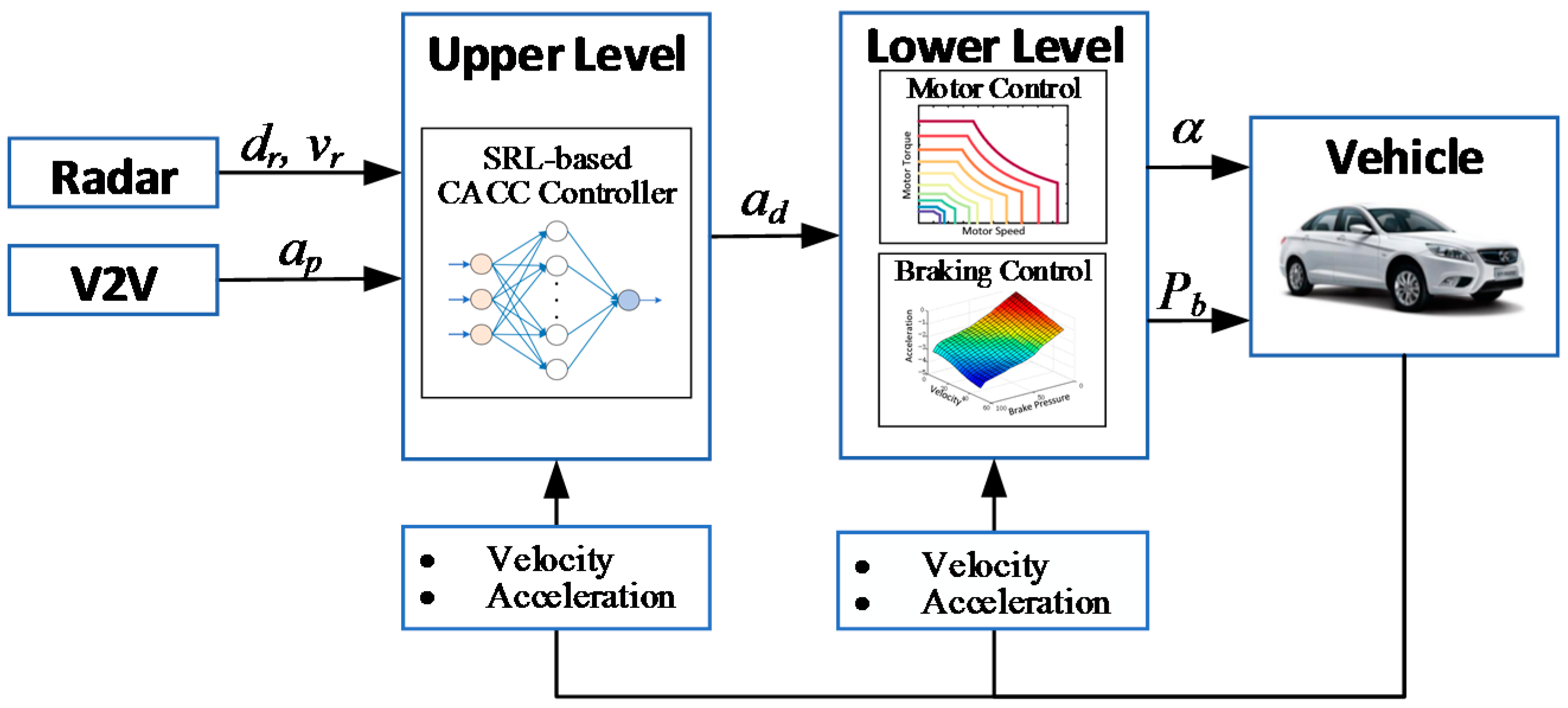
2.1. Control Framework for CACC
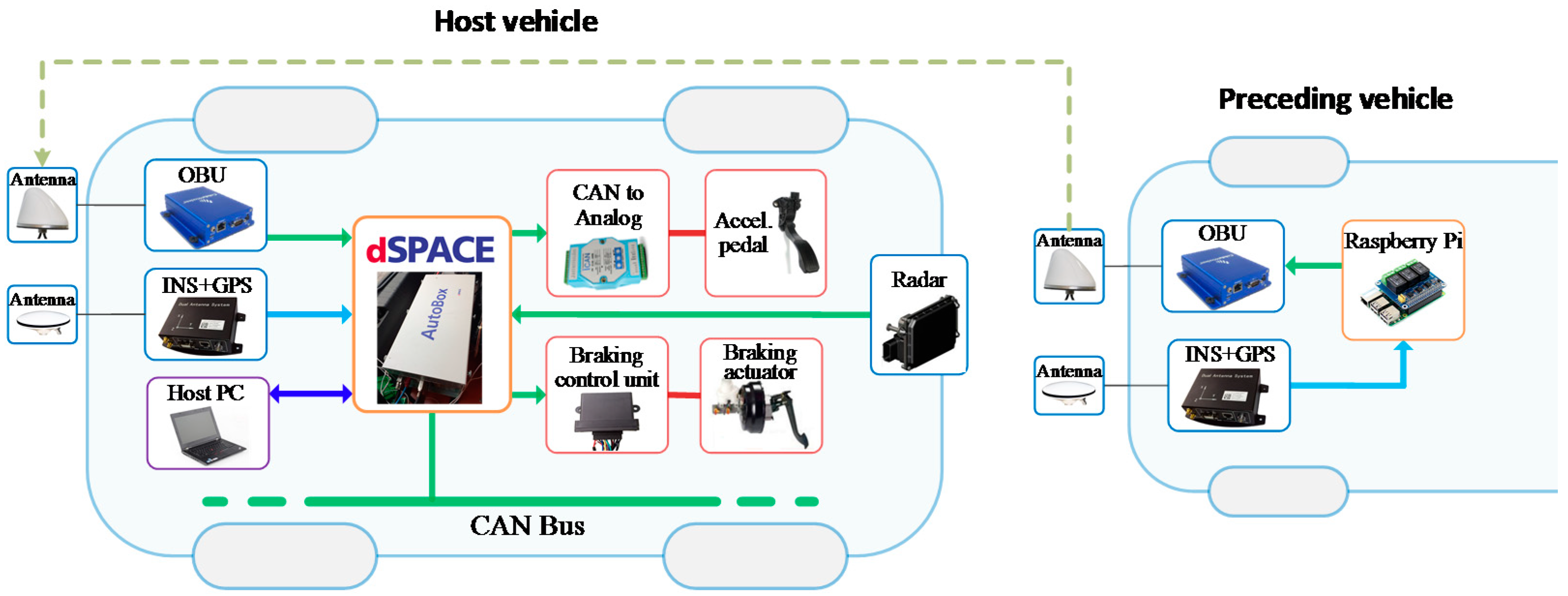
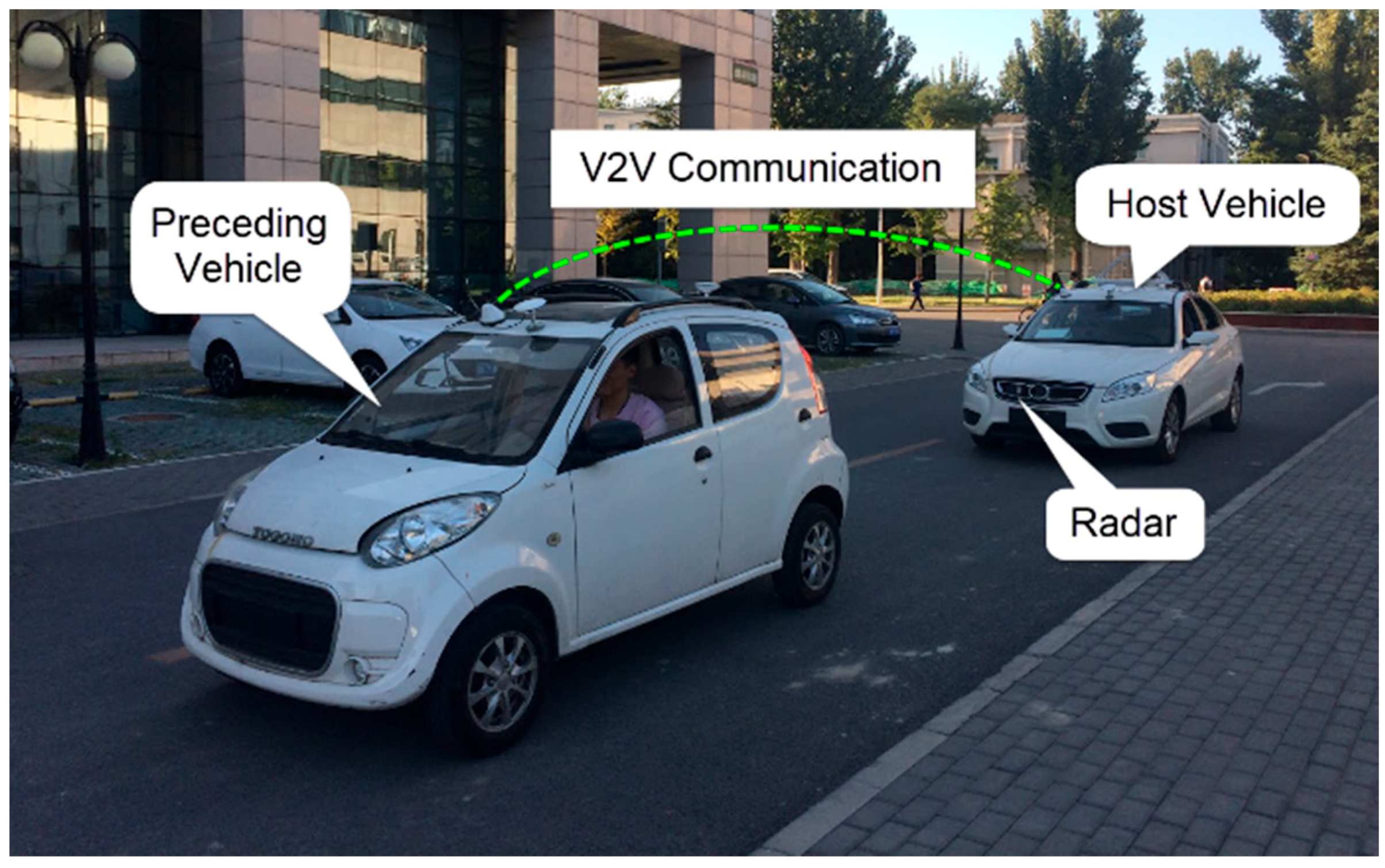
2.2. Hardware Implementation for the Test Platform
3. The SRL-Based Control Strategy for CACC
3.1. System Dynamics
3.2. The SRL Control Algorithm
3.2.1. The Actor Network
3.2.2. The Critic Network
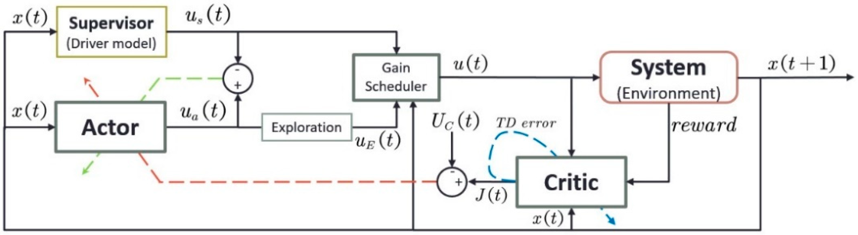
3.2.3. The Supervisor
3.2.4. The Gain Scheduler
3.2.5. SRL Learning
| Algorithm 1. Supervised Reinforcement Learning algorithm. |
| 1: Collect driving samples from a human driver in an infinite time horizon |
| 2: Train the supervisor network with using the Levenberg-Marquardt method |
| 3: Input the actor and critic learning rate ; the discount factor ; the exploration size ; and the interpolation parameter |
| 4: Initialize the weights of the actor and critic randomly |
| 5: Repeat for each trial |
| 6: initial state of the trial |
| 7: repeat for each step of the trial |
| 8: action given by the supervisor |
| 9: action given by the actor |
| 10: |
| 11: interpolation parameter from the gain scheduler |
| 12: |
| 13: execute action and observe the reward and new state |
| 14: |
| 15: update the weights of the critic by (16) and (17) |
| 16: |
| 17: |
| 18: update the weights of the actor by (18), (23) and (24) |
| 19: |
| 20: until is terminal |
4. Experiment Results and Discussion
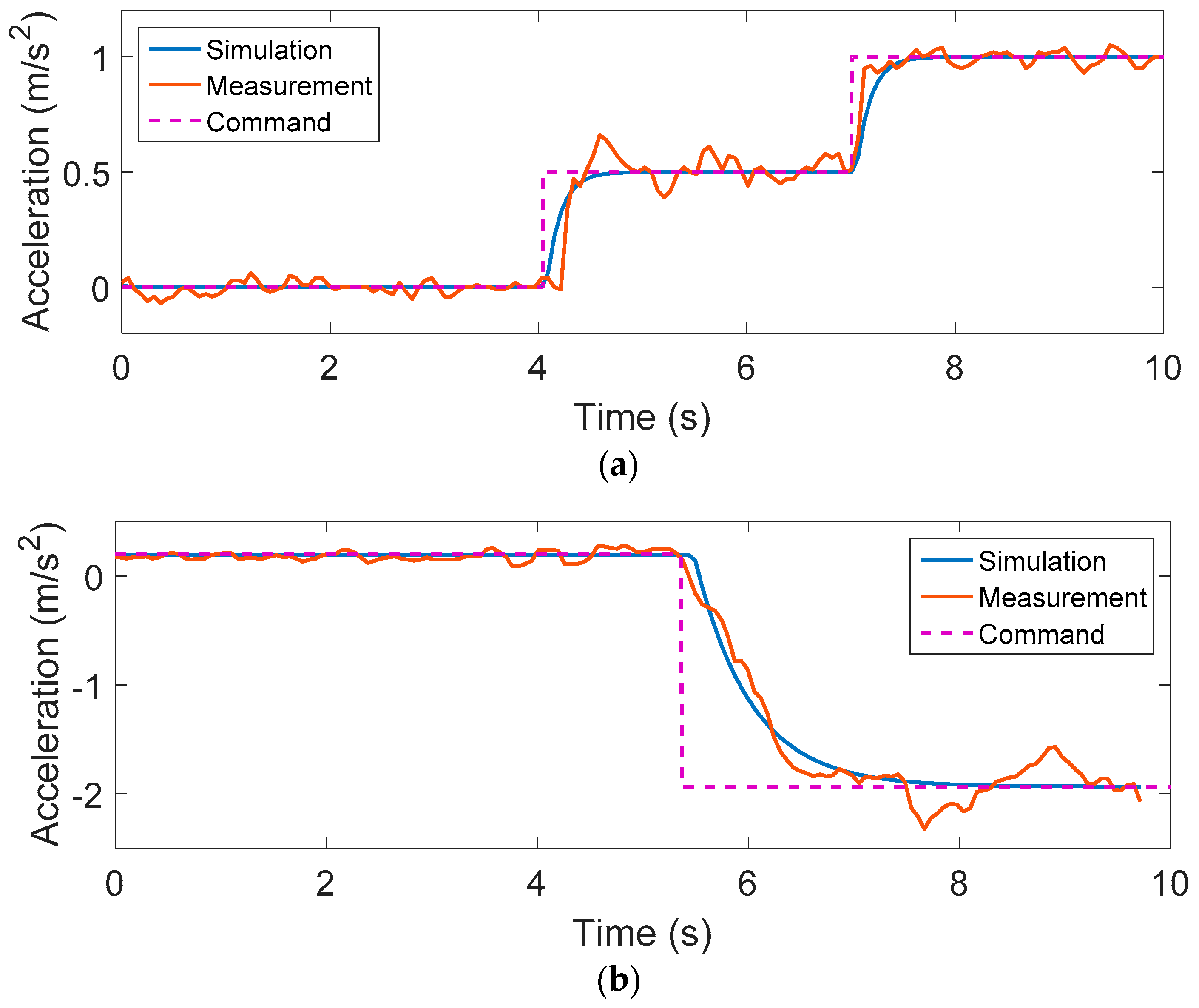
4.1. Vehicle Model Validation
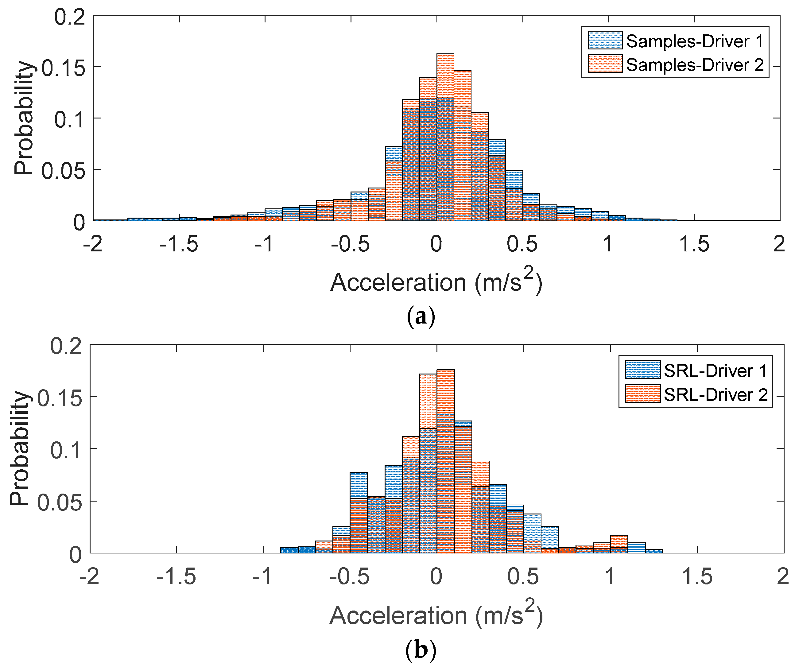
4.2. Training Process
4.3. Simulation Results
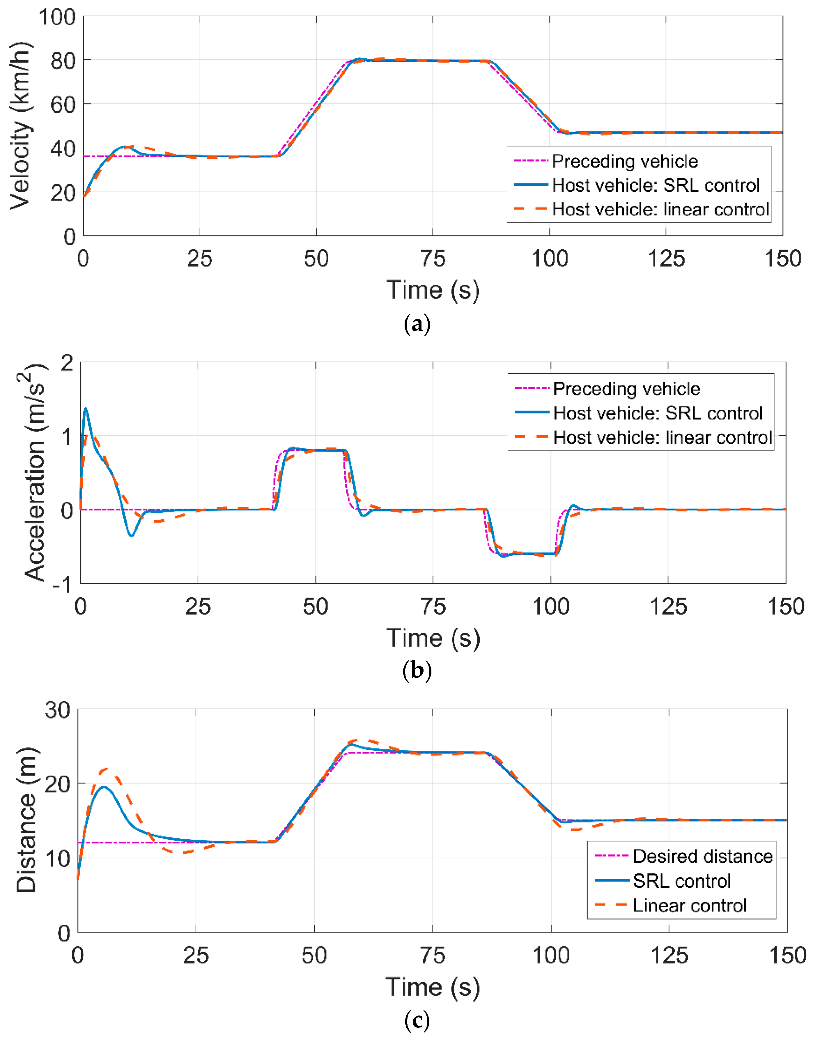
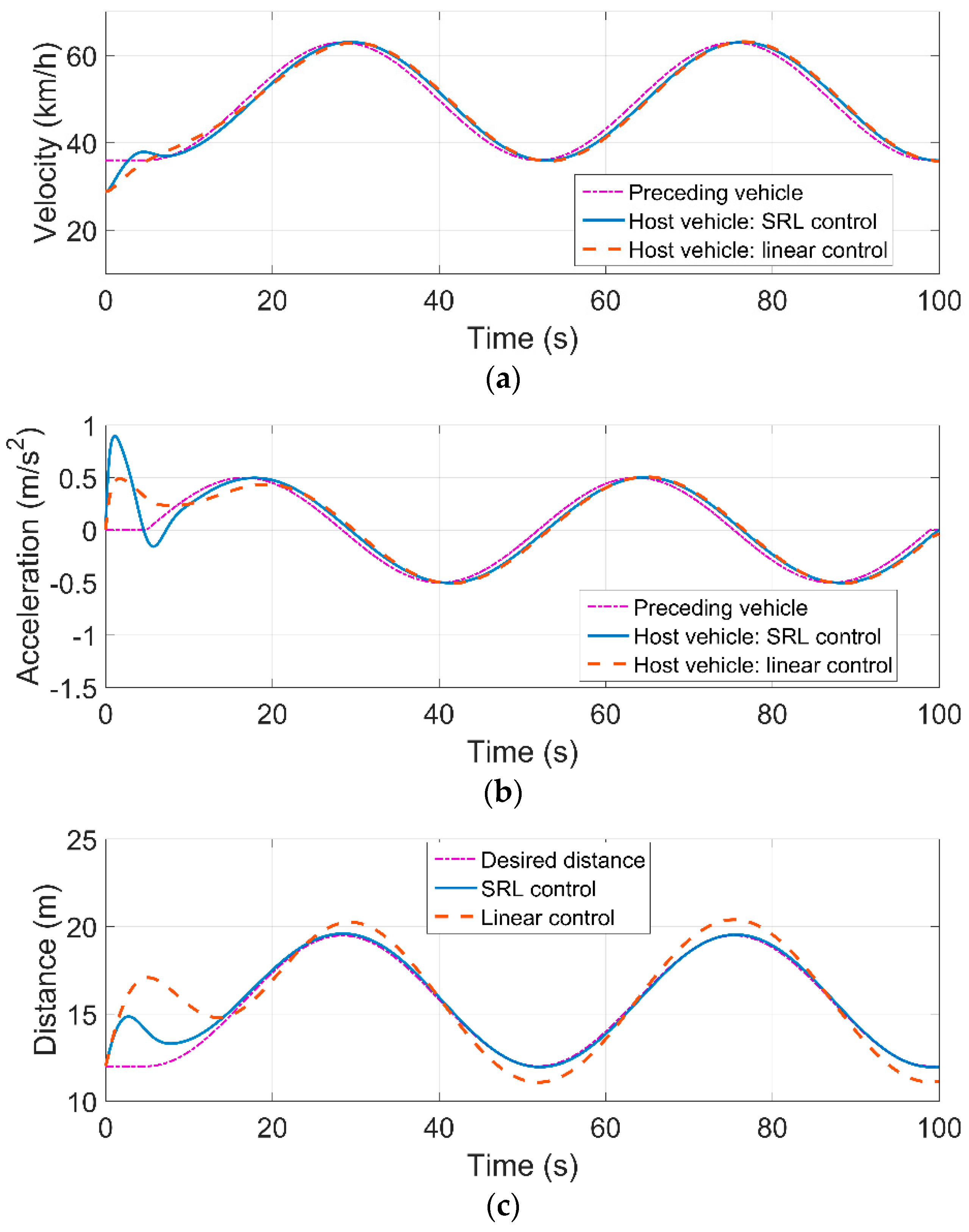
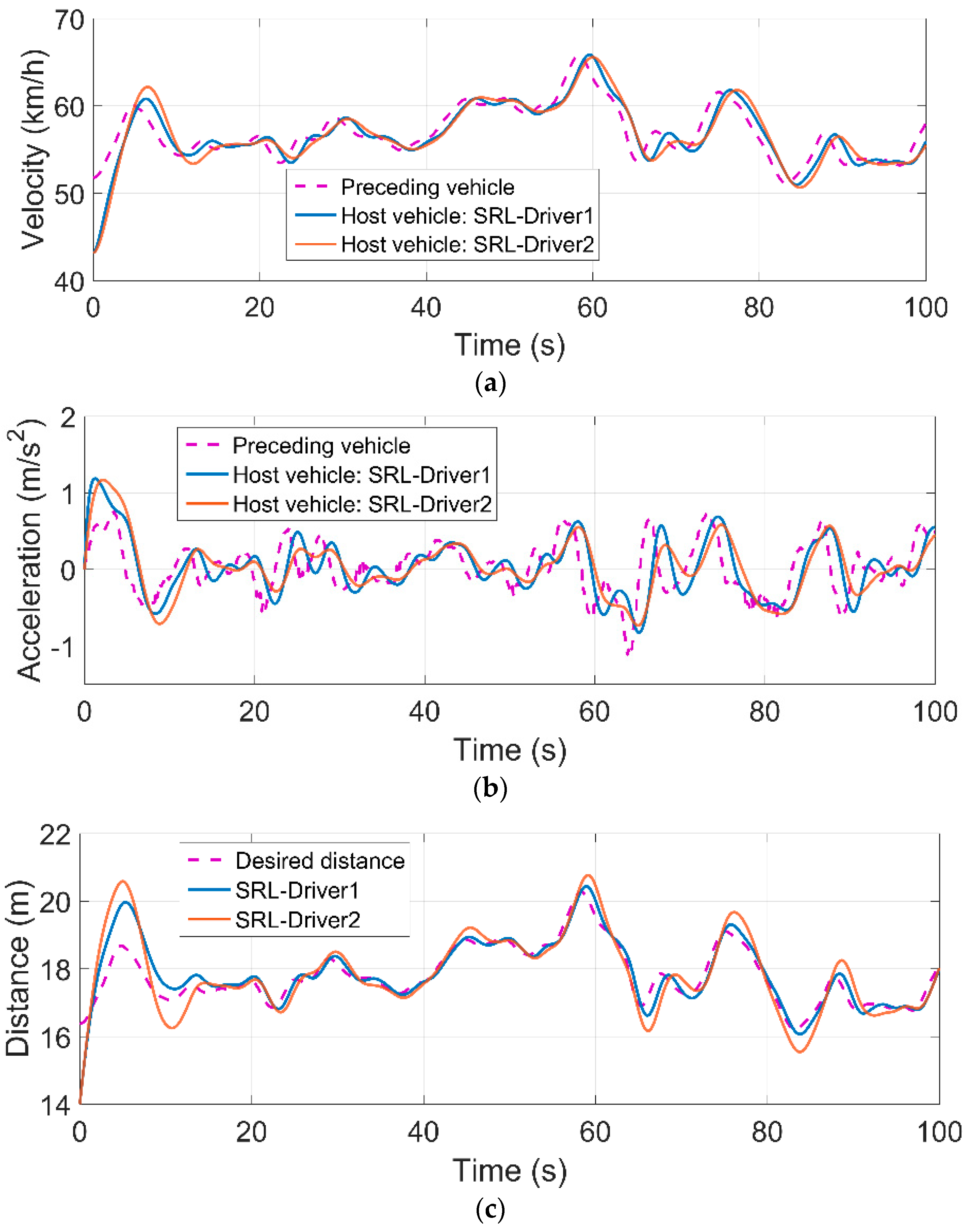
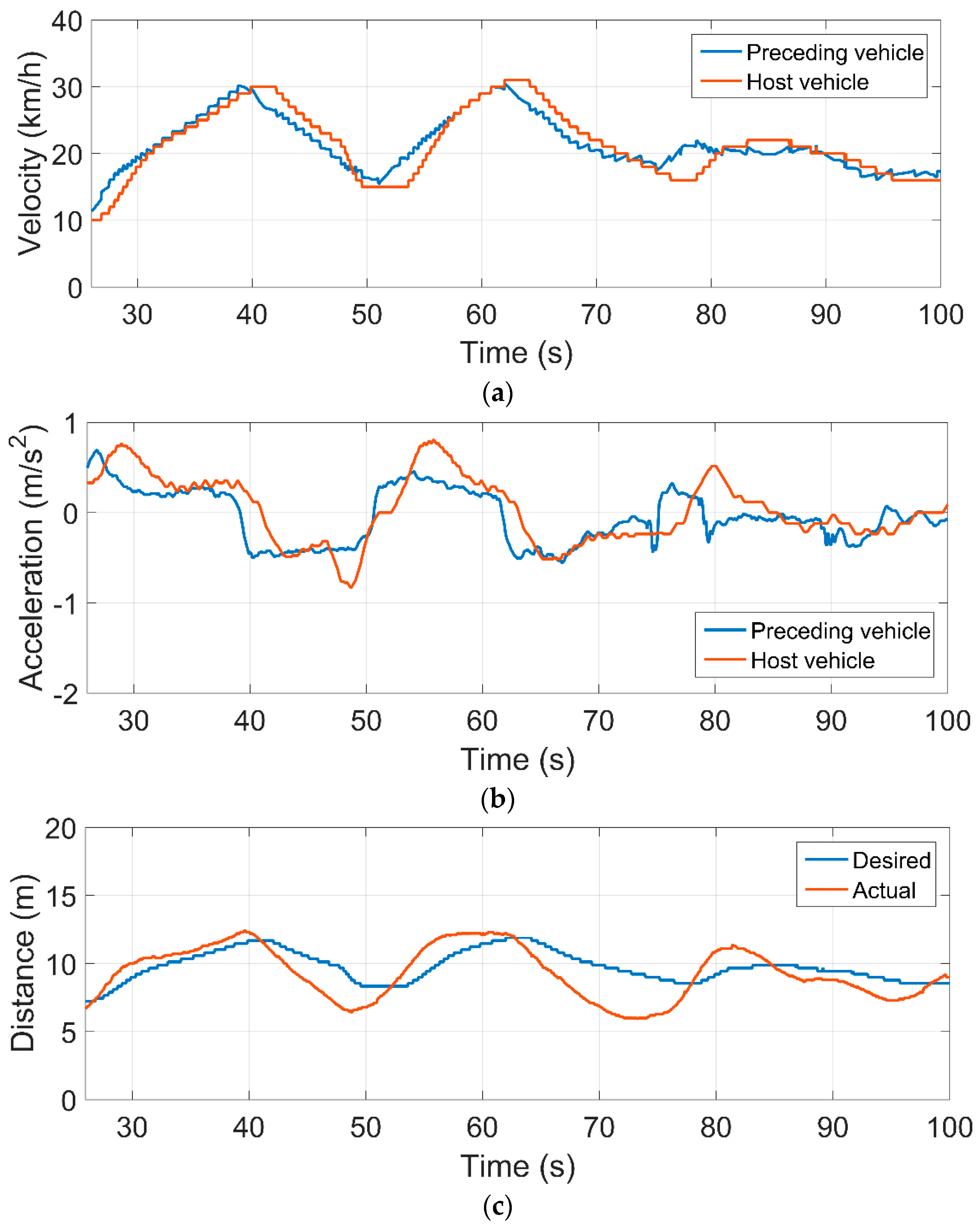
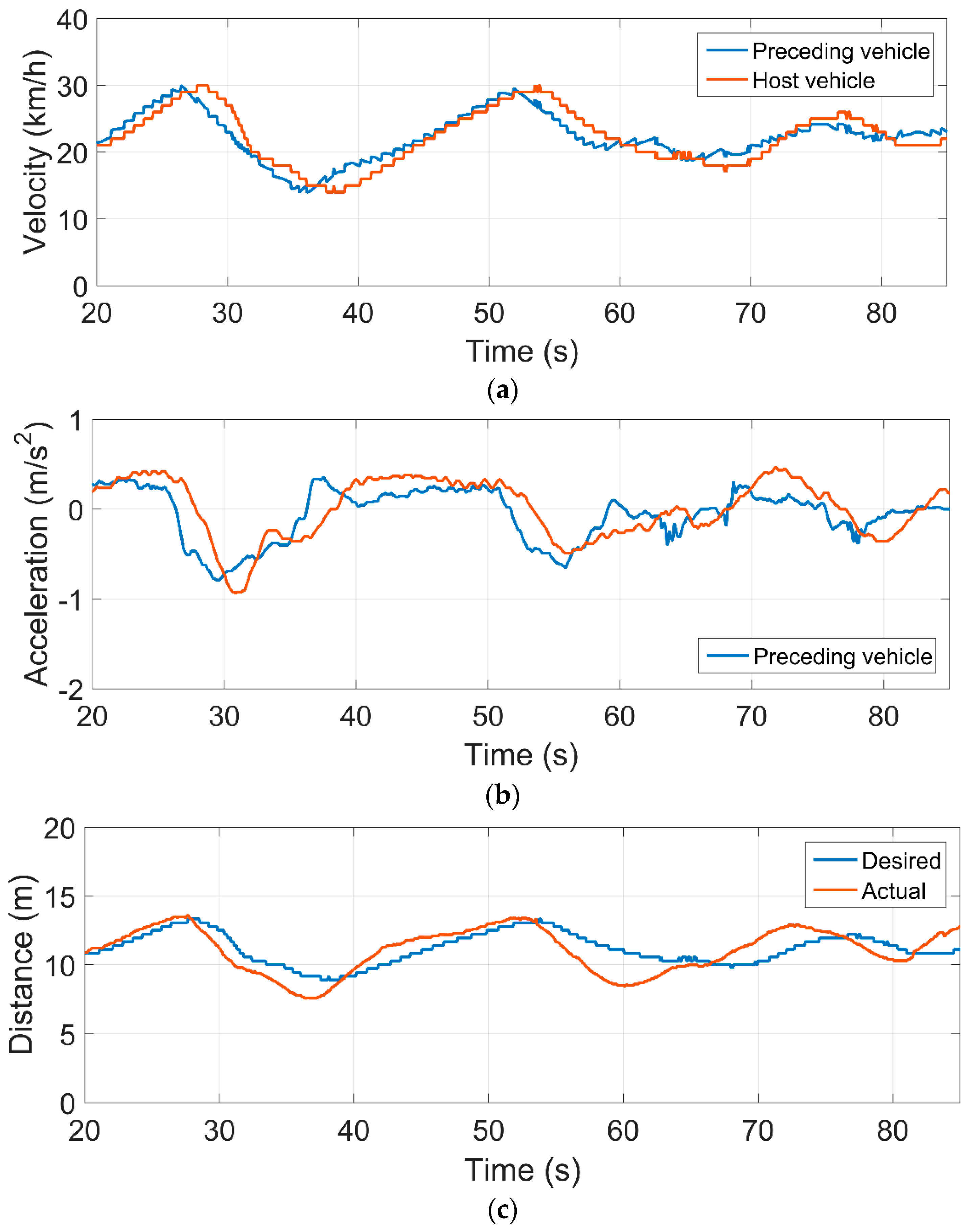
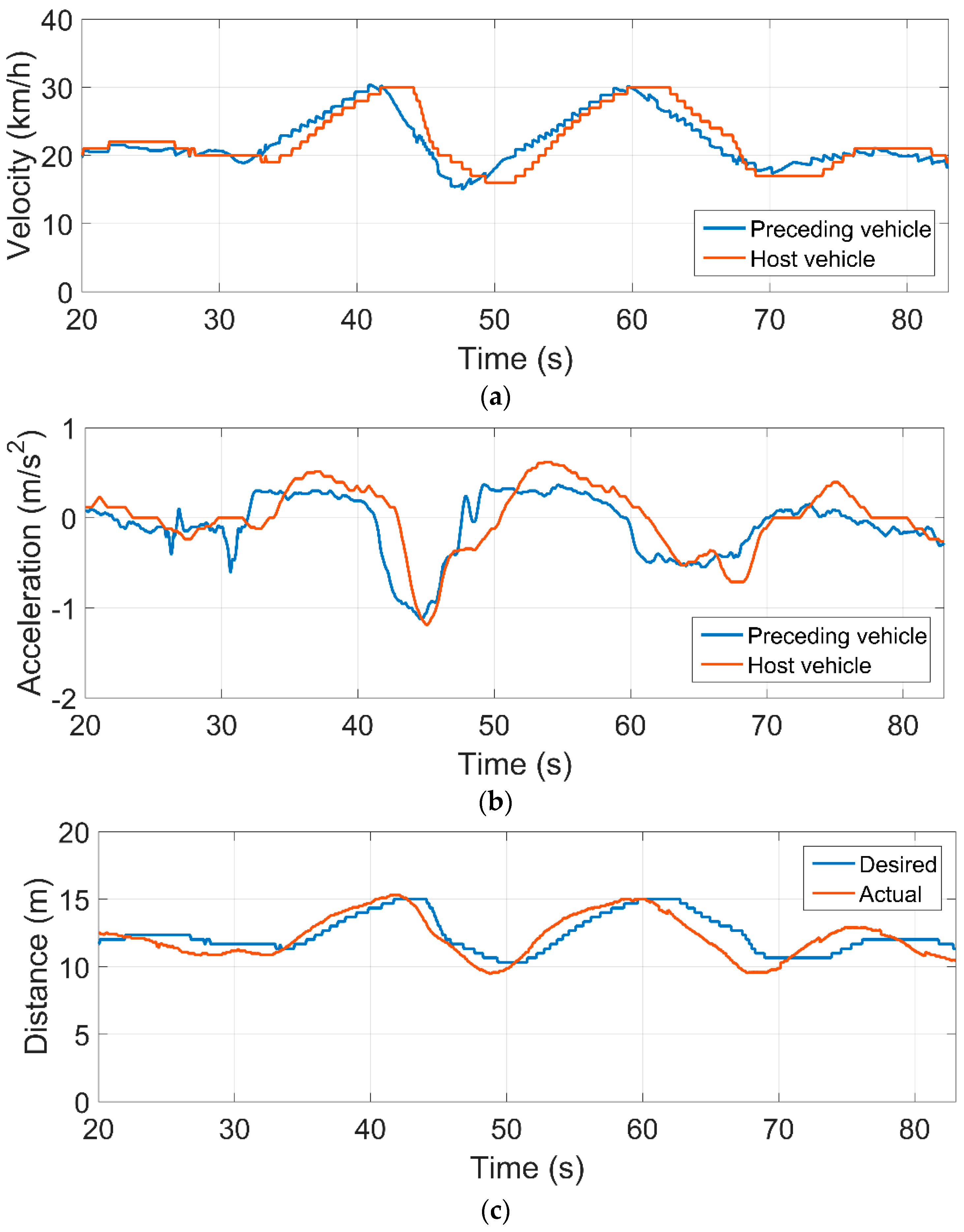
4.4. Test Results
5. Conclusions
Author Contributions
Funding
Conflicts of Interest
References
- 2013 Motor Vehicle Crashes: Overview, USDOT. Available online: https://crashstats.nhtsa.dot.gov/Api/Public/ViewPublication/812318 (accessed on 1 May 2018).
- National Bureau of Statistics of the PR China. 2016 China Statistical Yearbook. Available online: http://www.stats.gov.cn/tjsj/ndsj/2016/indexch.htm (accessed on 1 May 2018).
- Maimaris, A.; Papageorgiou, G. A review of Intelligent Transportation Systems from a communications technology perspective. In Proceedings of the 2016 IEEE 19th International Conference on Intelligent Transportation Systems (ITSC), Rio de Janeiro, Brazil, 1–4 November 2016; pp. 54–59. [Google Scholar]
- Zhang, J.; Wang, F.Y.; Wang, K.; Lin, W.H.; Xu, X.; Chen, C. Data-Driven Intelligent Transportation Systems: A Survey. IEEE Trans. Intell. Transp. Syst. 2011, 12, 1624–1639. [Google Scholar] [CrossRef]
- Moon, S.; Moon, I.; Yi, K. Design, tuning, and evaluation of a full-range adaptive cruise control system with collision avoidance. Control Eng. Pract. 2009, 17, 442–455. [Google Scholar] [CrossRef]
- Karagiannis, G.; Altintas, O.; Ekici, E.; Heijenk, G.; Jarupan, B.; Lin, K.; Weil, T. Vehicular Networking: A Survey and Tutorial on Requirements, Architectures, Challenges, Standards and Solutions. IEEE Commun. Surv. Tutor. 2011, 13, 584–616. [Google Scholar] [CrossRef]
- Chen, S.; Hu, J.; Shi, Y.; Zhao, L. LTE-V: A TD-LTE-Based V2X Solution for Future Vehicular Network. IEEE Internet Things 2016, 3, 997–1005. [Google Scholar] [CrossRef]
- Li, S.E.; Zheng, Y.; Li, K.; Wu, Y.; Hedrick, J.K.; Gao, F.; Zhang, H. Dynamical Modeling and Distributed Control of Connected and Automated Vehicles: Challenges and Opportunities. IEEE Intell. Transp. Syst. 2017, 9, 46–58. [Google Scholar] [CrossRef]
- Dey, K.C.; Yan, L.; Wang, X.; Wang, Y.; Shen, H.; Chowdhury, M.; Yu, L.; Qiu, C.; Soundararaj, V. A Review of Communication, Driver Characteristics, and Controls Aspects of Cooperative Adaptive Cruise Control (CACC). IEEE Trans. Intell. Transp. Syst. 2016, 17, 491–509. [Google Scholar] [CrossRef]
- Qin, W.B.; Gomez, M.M.; Orosz, G. Stability and frequency response under stochastic communication delays with applications to connected cruise control design. IEEE Trans. Intell. Transp. Syst. 2017, 18, 388–403. [Google Scholar] [CrossRef]
- Firooznia, A.; Ploeg, J.; van de Wouw, N.; Zwart, H. Co-design of Controller and Communication Topology for Vehicular Platooning. IEEE Trans. Intell. Transp. Syst. 2017, 18, 2728–2739. [Google Scholar] [CrossRef]
- Shladover, S.E.; Nowakowski, C.; Lu, X.Y.; Ferlis, R. Cooperative Adaptive Cruise Control (CACC) Definitions and Operating Concepts. Transp. Res. Rec. J. Transp. Res. Board 2015, 2489, 145–152. [Google Scholar] [CrossRef]
- Liu, H.; Kan, X.; Shladover, S.E.; Lu, X.Y.; Ferlis, R.E. Impact of Cooperative Adaptive Cruise Control on Multilane Freeway Merge Capacity. J. Intell. Transp. Syst. 2018, 22, 263–275. [Google Scholar] [CrossRef]
- Liu, H.; Kan, X.D.; Shladover, S.E.; Lu, X.Y. Using Cooperative Adaptive Cruise Control (CACC) to Form High-Performance Vehicle Streams: Simulation Results Analysis. Available online: https://escholarship.org/uc/item/31w2f555 (accessed on 6 June 2018).
- Rajamani, R.; Shladover, S.E. An experimental comparative study of autonomous and co-operative vehicle-follower control systems. Transp. Res. C Emerg. Technol. 2001, 9, 15–31. [Google Scholar] [CrossRef]
- Robinson, T.; Chan, E.; Coelingh, E. Operating platoons on public motorways: An introduction to the SARTRE platooning programme. In Proceedings of the 17th World Congress on Intelligent Transport Systems, Busan, Korea, 25–29 October 2010; Volume 1, p. 12. [Google Scholar]
- Solyom, S.; Coelingh, E. Performance Limitations in Vehicle Platoon Control. IEEE Intell. Transp. Syst. 2013, 5, 112–120. [Google Scholar] [CrossRef]
- Tsugawa, S.; Kato, S. Energy ITS: Another application of vehicular communications. IEEE Commun. Mag. 2010, 48, 120–126. [Google Scholar] [CrossRef]
- Kianfar, R.; Augusto, B.; Ebadighajari, A.; Hakeem, U.; Nilsson, J.; Raza, A.; Papanastasiou, S. Design and Experimental Validation of a Cooperative Driving System in the Grand Cooperative Driving Challenge. IEEE Trans. Intell. Transp. Syst. 2012, 13, 994–1007. [Google Scholar] [CrossRef]
- Kokogias, S.; Svensson, L.; Pereira, G.C.; Oliveira, R.; Zhang, X.; Song, X.; Mårtensson, J. Development of Platform-Independent System for Cooperative Automated Driving Evaluated in GCDC 2016. IEEE Trans. Intell. Transp. Syst. 2018, 19, 1277–1289. [Google Scholar] [CrossRef]
- Naus, G.J.L.; Vugts, R.P.A.; Ploeg, J.; Molengraft, M.J.G.; Steinbuch, M. String-Stable CACC Design and Experimental Validation: A Frequency-Domain Approach. IEEE Trans. Veh. Technol. 2010, 59, 4268–4279. [Google Scholar] [CrossRef]
- Lidström, K.; Sjoberg, K.; Holmberg, U.; Andersson, J.; Bergh, F.; Bjade, M.; Mak, S. A Modular CACC System Integration and Design. IEEE Trans. Intell. Transp. Syst. 2012, 13, 1050–1061. [Google Scholar] [CrossRef]
- Milanés, V.; Shladover, S.E.; Spring, J.; Nowakowski, C.; Kawazoe, H.; Nakamura, M. Cooperative Adaptive Cruise Control in Real Traffic Situations. IEEE Trans. Intell. Transp. Syst. 2014, 15, 296–305. [Google Scholar] [CrossRef]
- Geiger, A.; Lauer, M.; Moosmann, F.; Ranft, B.; Rapp, H.; Stiller, C.; Ziegler, J. Team AnnieWAY’s Entry to the 2011 Grand Cooperative Driving Challenge. IEEE Trans. Intell. Transp. Syst. 2012, 13, 1008–1017. [Google Scholar] [CrossRef]
- Wang, P.; Sun, Z.; Tan, J.; Huang, Z.; Zhu, Q.; Zhao, W. Development and evaluation of Cooperative Adaptive Cruise Controllers. In Proceedings of the 2015 IEEE International Conference on Mechatronics and Automation (ICMA), Beijing, China, 2–5 August 2015; pp. 1607–1612. [Google Scholar]
- Zheng, Y.; Li, S.E.; Li, K.; Borrelli, F.; Hedrick, J.K. Distributed Model Predictive Control for Heterogeneous Vehicle Platoons under Unidirectional Topologies. IEEE Trans. Control Syst. Technol. 2017, 25, 899–910. [Google Scholar] [CrossRef]
- Hu, X.; Wang, H.; Tang, X. Cyber-Physical Control for Energy-Saving Vehicle Following with Connectivity. IEEE Trans. Ind. Electron. 2017, 64, 8578–8587. [Google Scholar] [CrossRef]
- Rahman, M.; Chowdhury, M.; Dey, K.; Islam, R.; Khan, T. An Evaluation Strategy for Driver Car-Following Behavior Models for CACC Controllers. Transportation Research Board. 2017. Available online: https://trid.trb.org /view/1439218 (accessed on 1 May 2018).
- Wang, X.; Wang, Y. Human-aware autonomous control for cooperative adaptive cruise control (CACC) systems. In Proceedings of the ASME 2015 Dynamic Systems and Control Conference, Columbus, OH, USA, 28–30 October 2015; p. V002T31A001. [Google Scholar]
- Sutton, R.S.; Barto, A.G. Reinforcement Learning: An Introduction; MIT Press: Cambridge, UK, 1998. [Google Scholar]
- Xu, X.; Liu, C.; Hu, D. Continuous-action reinforcement learning with fast policy search and adaptive basis function selection. Soft Comput. 2011, 15, 1055–1070. [Google Scholar] [CrossRef]
- Kober, J.; Bagnell, J.A.; Peters, J. Reinforcement learning in robotics: A survey. Int. J. Robot. Res. 2013, 32, 1238–1274. [Google Scholar] [CrossRef]
- Liu, T.; Zou, Y.; Liu, D.; Sun, F. Reinforcement Learning of Adaptive Energy Management with Transition Probability for a Hybrid Electric Tracked Vehicle. IEEE Trans. Ind. Electron. 2015, 62, 7837–7846. [Google Scholar] [CrossRef]
- Zhao, D.; Hu, Z.; Xia, Z.; Alippi, C.; Zhu, Y.; Wang, D. Full-range adaptive cruise control based on supervised adaptive dynamic programming. Neurocomputing 2014, 125, 57–67. [Google Scholar] [CrossRef]
- Zhao, D.; Wang, B.; Liu, D. A supervised Actor–Critic approach for adaptive cruise control. Soft Comput. 2013, 17, 2089–2099. [Google Scholar] [CrossRef]
- Desjardins, C.; Chaib-draa, B. Cooperative Adaptive Cruise Control: A Reinforcement Learning Approach. IEEE Trans. Intell. Transp. Syst. 2011, 12, 1248–1260. [Google Scholar] [CrossRef]
- Huang, Z.; Xu, X.; He, H.; Tan, J.; Sun, Z. Parameterized Batch Reinforcement Learning for Longitudinal Control of Autonomous Land Vehicles. IEEE Trans. Syst. Man. Cybern. Syst. 2017, 99, 1–12. [Google Scholar] [CrossRef]
- Barto, M.; Rosenstein, M.T. Supervised Actor-critic Reinforcement Learning. In Handbook of Learning and Approximate Dynamic Programming; John Wiley & Sons: Toronto, ON, Canada, 2004; Volume 2, p. 359. [Google Scholar]
- Si, J.; Wang, Y.T. Online learning control by association and reinforcement. IEEE Trans. Neural Netw. 2001, 12, 264–276. [Google Scholar] [CrossRef] [PubMed]
- Wang, F.Y.; Zhang, H.; Liu, D. Adaptive Dynamic Programming: An Introduction. IEEE Comput. Intell. Mag. 2009, 4, 39–47. [Google Scholar] [CrossRef]
- Xiao, L.; Gao, F. Practical String Stability of Platoon of Adaptive Cruise Control Vehicles. IEEE Trans. Intell. Transp. Syst. 2011, 12, 1184–1194. [Google Scholar] [CrossRef]
- Lefèvre, S.; Sun, C.; Bajcsy, R.; Laugier, C. Comparison of parametric and non-parametric approaches for vehicle speed prediction. In Proceedings of the 2014 American Control Conference, Portland, OR, USA, 4–6 June 2014; pp. 3494–3499. [Google Scholar]
- Lin, Y.; Tang, P.; Zhang, W.; Yu, Q. Artificial neural network modelling of driver handling behaviour in a driver-vehicle-environment system. Int. J. Veh. Des. 2005, 37, 24–45. [Google Scholar] [CrossRef]
- Chong, L.; Abbas, M.M.; Flintsch, A.M.; Higgs, B. A rule-based neural network approach to model driver naturalistic behavior in traffic. Transp. Res. C Emerg. Technol. 2013, 32, 207–223. [Google Scholar] [CrossRef]
- Feng, L.; Sun, J.; Si, J.; Gao, W.; Mei, S. A boundedness result for the direct heuristic dynamic programming. Neural Netw. 2012, 32, 229–235. [Google Scholar]


| Algorithm | Number of Experiments | Success Rate | Average Number of Trials |
|---|---|---|---|
| SRL | 100 | 100% | 128 |
| RL | 100 | 34% | 724 |
| Control Policy | Maximum (m) | Average (m) | Variance |
|---|---|---|---|
| SRL control | 7.50 | 0.48 | 2.05 |
| Linear control | 9.86 | 0.52 | 4.57 |
| Control Policy | Maximum (m) | Average (m) | Variance |
|---|---|---|---|
| SRL control | 2.84 | 0.23 | 0.31 |
| Linear control | 5.07 | 0.43 | 1.83 |
| Control Policy | Maximum (m) | Average (m) | Variance |
|---|---|---|---|
| SRL-Driver1 | 1.39 | 0.08 | 0.13 |
| SRL-Driver2 | 1.93 | 0.05 | 0.30 |
| Time Headway (s) | Maximum (m) | Average (m) | Variance |
|---|---|---|---|
| 0.8 | 3.41 | −0.43 | 2.01 |
| 1.0 | 2.54 | −0.12 | 1.24 |
| 1.2 | 2.50 | −0.10 | 0.95 |
© 2018 by the authors. Licensee MDPI, Basel, Switzerland. This article is an open access article distributed under the terms and conditions of the Creative Commons Attribution (CC BY) license (http://creativecommons.org/licenses/by/4.0/).
Share and Cite
Wei, S.; Zou, Y.; Zhang, T.; Zhang, X.; Wang, W. Design and Experimental Validation of a Cooperative Adaptive Cruise Control System Based on Supervised Reinforcement Learning. Appl. Sci. 2018, 8, 1014. https://doi.org/10.3390/app8071014
Wei S, Zou Y, Zhang T, Zhang X, Wang W. Design and Experimental Validation of a Cooperative Adaptive Cruise Control System Based on Supervised Reinforcement Learning. Applied Sciences. 2018; 8(7):1014. https://doi.org/10.3390/app8071014
Chicago/Turabian StyleWei, Shouyang, Yuan Zou, Tao Zhang, Xudong Zhang, and Wenwei Wang. 2018. "Design and Experimental Validation of a Cooperative Adaptive Cruise Control System Based on Supervised Reinforcement Learning" Applied Sciences 8, no. 7: 1014. https://doi.org/10.3390/app8071014
APA StyleWei, S., Zou, Y., Zhang, T., Zhang, X., & Wang, W. (2018). Design and Experimental Validation of a Cooperative Adaptive Cruise Control System Based on Supervised Reinforcement Learning. Applied Sciences, 8(7), 1014. https://doi.org/10.3390/app8071014