Featured Application
Multiwavelength digital holography on objects beyond the unambiguous measurement range.
Abstract
Digital holography is a well-established technology for optical quality control in industrial applications. Two common challenges in digital holographic measurement tasks are the ambiguity at phase steps and the limited depth of focus. With multiwavelength holography, multiple artificial wavelengths are used to extend the sensor’s measurement range up to several millimeters, allowing measurements on rough surfaces. To further extend the unambiguous range, additional highly stabilized and increasingly expensive laser sources can be used. Besides that, unwrapping algorithms can be used to overcome phase ambiguities—but these require continuous objects. With the unique feature of numerical refocusing, digital holography allows the numerical generation of an all-in-focus unambiguous image. We present a shape-from-focus algorithm that allows the extension of the depth of field beyond geometrical imaging limitations and yields unambiguous height information, even across discontinuities. Phase noise is used as a focus criterion and to generate a focus index map. The algorithm’s performance is demonstrated at a gear flank with steep slopes and a step sample with discontinuities far beyond the system’s geometrical limit. The benefit of this method on axially extended objects is discussed.
1. Introduction
Quickly measuring three-dimensional (3D) surfaces with small 3D structures is a challenge for industrial measurement technology. For 100% inline-inspection of components, the measuring system has to keep up with the production cycle. Because of its great resolution and high speed, digital holography is a well-established technology for nondestructive testing in industrial applications [1,2,3,4,5,6,7]. Millions of data points can be acquired in a fraction of a second, which allows measuring cycles of multiple Hz.
Lateral resolution of holographic sensors is limited by the pixel pitch of the imaging device and designed magnification. With the use of a lens, it can be both improved and adapted. With respect to axial resolution and unambiguity, the wavelength of the laser and the dynamic range of the imaging device are limiting factors. In addition, limited depth-of-focus is a challenge addressed by our algorithm. Spatial unwrapping allows to extend the measuring range, but often fails (e.g., at steep edges and deep holes) [8]. Using digital multiwavelength holography, speckle fields are captured at identical boundary conditions but at different wavelengths. This allows a numerical generation of phase maps of an artificial wavelength. These generated synthetic wavefronts overcome both restrictions [9,10,11,12,13,14,15,16]. As an alternative to the additional expensive lasers and further appropriate longer synthetic wavelengths, the axial measurement range in digital holography can be extended using shape-from-focus algorithms for focus detection, applied on amplitude or phase images. Promising approaches have been highly investigated in the past (e.g., amplitude stack [17], complex ratio [18], correlation coefficient [19], energy conservation [19,20], entropy [19], Fourier spectral [19,20,21,22], Gini index [23], gradient [22], Kirchhoff [24], L1 norm [23,25], Laplacian [21,22,26], multispectral images [19,27], self-entropy [28], speckle phase decorrelation [29], Tamura coefficient [30,31] variance [19,21,26,32,33] Klicken oder tippen Sie hier, um Text einzugeben, quadratic deformation of spatial coordinates [34], cubic phase plate [35], amplitude modulus [36], or numerical axicon transformation [37]).
We present a shape-from-focus algorithm based on phase noise and use its output as a rough estimate of the object’s surface shape, which allows us to extend the measurement range far beyond the limits of synthetic wavelengths and geometrical depth-of-focus. This algorithm has been previously introduced by us in 2017 [38], using a maximum filter in combination with a plane fit for height map generation. In this paper, we present a generalized improvement using a pixel wise Gaussian fit.
The performance of our method is demonstrated using a gear test object at steep slopes and a step object with gaps beyond the measuring unambiguous range. Even at steep slopes, we are able to numerically compute an all-in-focus image of the gear flank beyond the measurement range of the synthetic wavelengths being used. In order to save computing time, data processing is mostly executed on the graphics processing unit (GPU).
2. Experimental Setup
Figure 1a shows an experimental setup for multiwavelength digital holography with an exemplary gear tooth. However, the algorithm introduced in this paper is not limited to this setup, but is applicable to holographic setups in general. A detailed description of our optical setup has been introduced by the authors of [38].
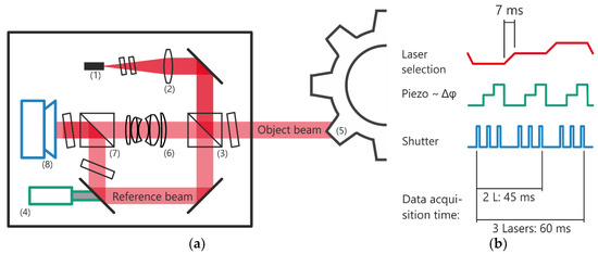
Figure 1.
Experimental setup for temporal phase-shifting multiwavelength digital holography: (a) sensor internals including laser system (1); lens (2); polarizing beam splitter cubes (3)/(7); piezo (4); camera (8); gear test object (5); and imaging lens (6). The interferometric optical path includes reference and object beams, which are superimposed on the imaging device. Lenses (2) and (6) ensure maximal light yield; (b) data acquisition time series using three lasers and three piezo steps for temporal phase shifting. In total, nine camera images are acquired.
Three separate grating-stabilized diode lasers (632.9443 nm, 636.2661 nm, and 635.8239 nm) are used. The typical linewidth of the individual laser is specified to be between 0.5 and 1 MHz. With two wavelengths, and , the artificial wavelengths , as follows,
can be calculated to 915 µm, 140 µm, and 121 µm. The different lasers are connected through a fiber switch to the interferometer. Only one wavelength is present in the sensor at a time. To ensure a common source point, single-mode fibers are used to connect the lasers (1) to the sensor. The beam is split into reference and object beam by a polarizing beam splitter cube (3). By rotating the angle of the polarizing-maintaining fiber, the ratio between the beams can be adjusted. Later, the orthogonally polarized beams are combined without losses by the second polarizing beam splitter cube. For the reference beam path, an achromatic lens (2) converts the beam to a convergent beam with an interim focus on the piezo (4). Having passed a polarizing beam splitter cube (7), the beam is deflected onto the camera (8). For temporal phase shifting, the piezo introduces a minimum of three phase steps by an angle of approximately , respectively. The piezo runs in an open-loop mode and the exact phase-steps are calculated subsequently (Section 3) [1,39]. Passing a polarizing beam splitter cube (3), the object beam is reflected by the sample (5), and focused onto the camera by an imaging lens (6) as an interference pattern.
Figure 1b shows the measurement data acquisition time series for our three laser setup at three phase steps . With this configuration, the data acquisition for one measurement takes 60 ms and includes nine raw images.
3. Algorithm
The numerical reconstruction of the all-in-focus height map is performed in four steps, as follows:
- Temporal phase-shifting–determination of the global phase shifts between single images induced by the piezoactuator and the calculation of the complex wave [39,40,41].
- Propagation of the complex wave and calculation of the synthetic wavefronts [39].
- Shape-from-focus (described in this section):
- Maximum filter (Section 3.1) [38]
- Gaussian fit (Section 3.2)
- Iterative combination of focus criterion and finer artificial wavelengths [15,38].
We propose a method to calculate an extended focus image based on the phase noise, and combine the respective synthetic wavefronts using this output of the algorithm.
As input data, the phase information at arbitrary (even multiple) wavelengths can be processed. A pre-filter with radius 2 has been found to effectively reduce camera noise on the complex holograms. Firstly, the phase noise and in and direction of a synthetic wavefront at reconstruction distance , is calculated.
The gradient vector
can be normalized as follows:
With a moving average filter (e.g., radius = 8), the amplitude of the phase smoothness for each pixel at reconstruction distance is used as a focus criterion, as follows:
Figure 2 illustrates the principle of the algorithm graphically, as follows: Panel (a) shows a synthetic phase map with linearly increasing noise from left to right. Panel (b) shows the anisotropic normalized phase gradient for the low-noise (green) and high-noise (orange) areas, taken from the synthetic data in panel (a), respectively. Areas of low noise are characterized by a uniform phase gradient direction, whereas noisy areas appear as random phase vectors. In the following, we use a filtered sum of these gradient vectors , shown in panel (c), as our phase noise or rather, the phase smoothness criteria. It can be interpreted as the filtered information inside the moving average kernel. A large gradient vector sum indicates an area of smooth phase and thus focused pixel. In out-of-focus areas, the gradient vectors are noisy and the is shorter.
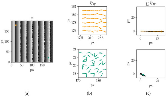
Figure 2.
Algorithm principle from phase map input to phase noise output. (a) Simulated phase map with linearly increasing noise from left to right; (b) phase gradient direction for low-noise and high-noise points in a 6 × 6 px2 area; and (c) sum of gradient direction vectors for low-noise (top) and high-noise (bottom) points. A long sum vector indicates an area of smooth phase.
Figure 3 shows the output of the algorithm at a single point , and different reconstruction distances for a gear sample. The graph clearly shows a maximum at around = 6 mm.
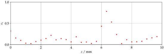
Figure 3.
Phase smoothness at different reconstruction distances for a gear sample. A maximum around 6 mm can be found, corresponding to the in-focus distance.
To find the in-focus distances within the stack of images at propagation distances , a minimum phase–noise value of the stack of calculated propagation distances for each pixel coordinate has to be found. In the following, two methods for the synthesis of a phase map with extended depth of field are proposed.
3.1. Maximum Filter
Previously, we used a similar phase–noise algorithm with pixel wise maximum filter data processing [38]. The maximum filter output can be calculated with a low computation effort and shows a very even yet discrete focusing map, as follows:
3.2. Gaussian Fit
Further investigations qualify the pixel wise Gaussian fit as a tremendous improvement. The results presented in Section 4 could be achieved by the following algorithm: all pixels of the shape-from-focus stack are used as sampling points for a pixel wise Gaussian fit with four degrees of freedom, as follows:
The fit is initialized using the distance of the maximum phase smoothness as a first estimate for the peak position , and c being the ground noise of the signal. The scaling parameter is initialized as the peak value of the maximum phase smoothness, along with the experimentally determined of 0.5, complete our initial parameters for up to 1000 iterations. The expected value of each Gaussian fit is used for the final focus map .
The values with a maximum phase smoothness below 0.3 are marked in a separate mask. The corresponding height
is used as a rough synthetic wavelength and serves as the starting information for the combination of further synthetic wavelengths.
In order to being able to use this method for inline-measurements, computation-intensive calculations are processed on the GPU, since pixel wise operations can be efficiently evaluated in parallel. Having transferred the complex holograms to the GPU, the phase noise, filtering, and Gaussian fitting are computed on the GPU.
4. Results
Unless otherwise stated, all calculations in this section are conducted on the finest synthetic wavelength at 121 µm.
4.1. Gear Tooth Sample
An evaluation of a gear tooth with an axial extension greater 5 mm is presented in this Section. Thirty equally spaced propagation distances from 0 mm to 10 mm have been calculated. Figure 4 shows our experimental setup, including the gear test sample.
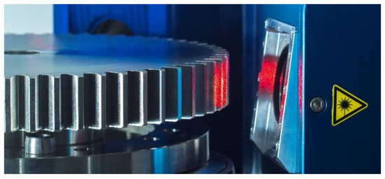
Figure 4.
Experimental setup including the gear tooth sample and holography sensor.
Figure 5 shows the phase (top) and phase smoothness (bottom) maps for two propagation distances = 3.0 mm and = 6.0 mm, respectively. For areas of low noise and thus focused parts, the phase shows sharp stripes, whereas the unfocused areas are superimposed by noise. In the left panels, a propagation distance of = 3.0 mm is pictured with the focused point and the associated phase smoothness on the right area of the measurement. The right panels were evaluated at a propagation distance of = 6.0 mm and show a clear maximum band and horizontally decreasing focus on the left of the measurement.
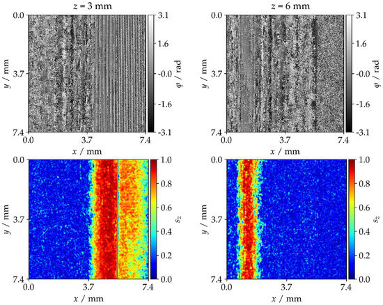
Figure 5.
Phase (left/right) and phase smoothness for two propagation distances . Left: = 3 mm, right: = 6 mm. Sharp stripes can be observed in areas of low phase noise, whereas areas of high phase noise appear as random phase distribution.
As a next step, the synthesis of phase maps with an extended depth of field has to be addressed—the calculated propagation stack holds a best phase–noise distance for each pixel coordinate . Figure 6 shows the progression of the phase–noise signal at different reconstruction distances for equally distributed points on the gear flank. Two thumbnails at = 3.50 mm (left) and = 6.33 mm (right) illustrate the position of the crosses on the sample near the focus or the orange cross (left) and the red cross (right).
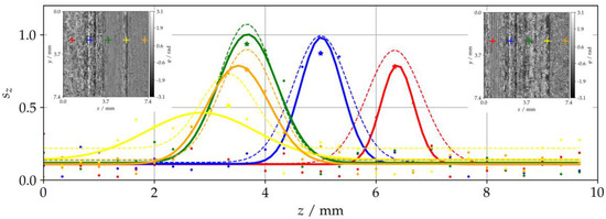
Figure 6.
Phase smoothness of several points at different propagation distances, . is marked with a , whereas can be read at the peak of the Gaussian fit. Two thumbnails at = 3.50 mm (left) and = 6.33 mm (right) illustrate the position of the crosses on the sample near the focus or the orange cross (left) and the red cross (right).
In the following sections, we propose two methods for the focus point selection with different applications.
4.1.1. Maximum Filter
Figure 7a shows the reconstruction distance at the maximum phase smoothness for each pixel. Since the shape-from-focus algorithm outputs the focus distance to the sample, its height information is inverse to the sample’s real surface. We note the inverse height information in the shape-from-focus output compared with the sample’s real surface. Except for the gear flank edge, the resulting height map shows a very smooth yet discrete focusing map. At the joint of both areas, a focus distance peak can be observed in Figure 7a. This outlier is due to a drop in the amplitude of in areas of low gradients, as shown at the yellow point in Figure 7b, which can lead to the wrong focus plane estimation.
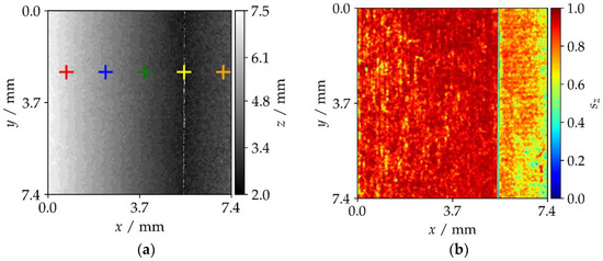
Figure 7.
Shape-from-focus output including phase smoothness as the quality criterion, high values show a strong result; (a) discrete focus map reconstructed by pixel wise shape-from-focus maximum. The sections at colored crosses are illustrated in Figure 6; (b) optimized values of using maximum filter.
4.1.2. Gaussian Fit
Using the Gaussian fit approach introduced in Section 3, we can overcome the discrete distribution and get the result shown in Figure 8a. The output now shows an even smoother progression with similar outliers at the gear flank edge. Using the amplitude of the phase gradient direction vectors, shown in Figure 8b, we get information about the signal quality, which can be used for weighted filtering.
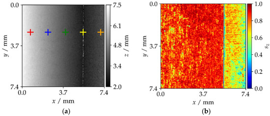
Figure 8.
Shape-from-focus output including phase smoothness as a quality criterion, high values show a strong result; (a) focus map reconstructed by pixel wise shape-from-focus Gaussian fit. The sections at colored crosses are illustrated in Figure 6; (b) optimized values of using the Gaussian approach.
Gaussian fits based on the sampling points, as described in Section 3, are plotted in Figure 6. The dashed-line shows the initial Gaussian fit guess for each point plotted in Figure 8a. The final Gaussian fits are shown as solid lines and are in very good agreement with the reconstruction distances.
Applied to all pixel values, both focus plane selections result in a continuously focused measurement, as shown in Figure 9.
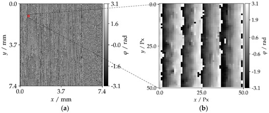
Figure 9.
(a) All-in-focus phase map –the whole measurement shows sharp stripes and minimized phase noise. In the 3072 × 3072 pixels original image, the fringes are clearly resolved; (b) Magnified view of the red area of (a). The fringe spacing is 10 pixels.
Now instead of using a very large synthetic wavelength, the shape-from-focus output can be used as rough estimation of the object’s surface shape for the combination of wavelengths. By combining the shape-from-focus data with all three synthetic wavelengths, we get the focused unambiguity-extended 3D results in Figure 10. However, due to the discrete progression of the shape-from-focus estimation, we get various combination errors applying finer wavelengths to the maximum filtered input data as shown in Figure 10a. Maximum filtered height estimation data works perfectly for all-in-focus calculations as shown in Figure 10 but has to be generated with very small propagation step width in order to suffice as a rough synthetic starting point for wavelength combination. Since this is very time-consuming, the Gaussian fit algorithm should be used instead here.
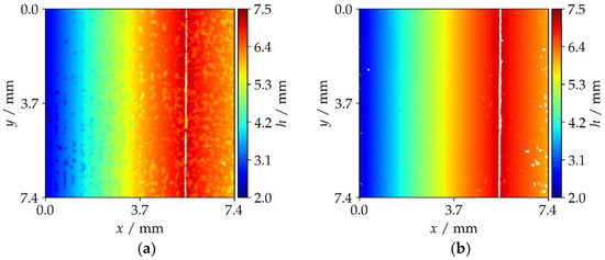
Figure 10.
Masked height map of the combined tooth data using (a) maximum filter: combination errors due to discrete and hence imprecise shape-from-focus data; (b) Gaussian filter: almost no combination errors occur onto the Gaussian fit output.
Applying all the finer wavelengths on the inverse of the Gaussian filter output, we get the focused unambiguity-extended 3D result in Figure 10b. The combined data considerably exceeds the geometrical ambiguity and focus limits, and is almost free of combination errors. is used in both of the height maps to mask out data points, but the shape-from-focus algorithm could not reconstruct safely. Masked data points are shown as white points.
4.2. Steps Sample
In this section, a tilted sample with discontinuous height steps larger than the measurement, the unambiguous range is evaluated. Figure 11a shows a photograph of this part, including a mm scale, and Figure 11b shows the sensor setup with the tilted step sample and its step height of 1.2 mm.
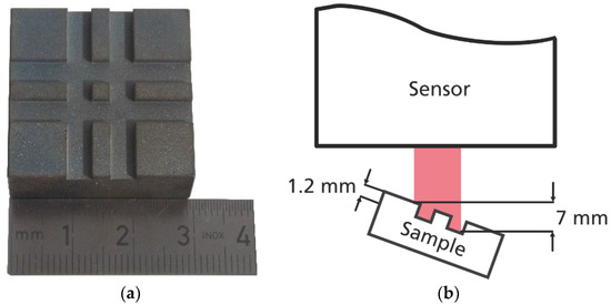
Figure 11.
(a) Photograph of step sample with discontinuous height steps beyond the sensor’s unambiguous range; (b) sketch of the sensor setup including the sample step height.
Figure 12a shows the shape-from-focus output using the superior Gaussian fit approach from Section 3.2. We were able to fully reconstruct the tilted sample very smoothly. However, because of two reasons, the edges of the plateaus show artefacts, as follows: Within the filter radius, we get mixed phase information and thus mixed values. Additionally, at very steep slopes, strong artefacts can be observed due to the stripes not being sufficiently sampled. These effects can be suppressed by additional weighted filtering.
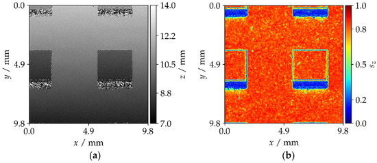
Figure 12.
Focus map reconstructed by pixel wise Gaussian fit to shape-from-focus output stack; (a) discrete focus map reconstructed by pixel wise shape-from-focus Gaussian fit; (b) optimized values of using the Gaussian filter. At very steep slopes, strong artefacts can be observed because of the stripes not being sufficiently sampled.
Figure 13 shows the combined height information for both filtering approaches. Even in a complex sample crossed by many steps far beyond the measurement’s unambiguous range, we get focused unambiguity-extended height information. For the maximum filter approach, the height map, as shown in panel (a), is disturbed by many combination errors. Conversely, the Gaussian filtered height map in panel (b) is almost free of combination errors.
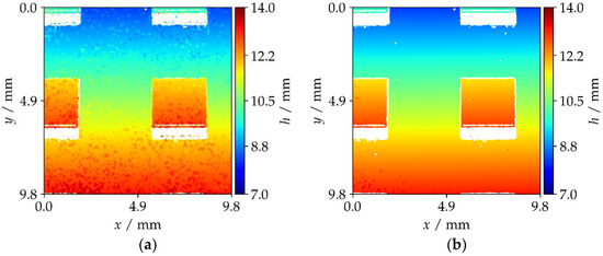
Figure 13.
Height map of the combined steps sample data using (a) maximum filter: combination errors due to discrete hence imprecise shape-from-focus data; (b) the Gaussian filter: almost no combination errors occur onto the Gaussian fit output.
5. Discussion
We presented a shape-from-focus algorithm for multi-wavelength holography using a phase noise measure, based on phase gradients. Firstly, a generic measuring setup for the application of this method was introduced. Two approaches (pixel wise maximum filter and the Gaussian fit on the shape-from-focus stack output) for the all-in-focus measurement data calculation were presented subsequently. The output of the algorithm is further used as a rough height estimation to overcome the phase ambiguities, and allows the extension of the unambiguous measurement range.
We were able to calculate an all-in-focus measurement and extend the range of unambiguousness beyond 12 mm at the largest synthetic wavelength of only 915 µm. In this range, we could not observe a decrease in signal quality. To date, no fundamental limit to the possible range are known. Using a setup with collimated illumination, experiments at meter-scale distances would be possible.
After having explained the algorithm in general, their respective performance at complex free-form surfaces was demonstrated. A gear tooth flank and a step sample at steep viewing angles demonstrate the performance of the algorithm. Both filters are able to reconstruct an all-in-focus phase map. However, only the Gaussian filter approach is able to reconstruct an unambiguity-free height map on top of the synthetic measurement data without combination errors.
Author Contributions
Conceptualization T.S., M.F., T.B., and A.S.; software and investigation, T.S., M.F., and T.B.; writing (original draft preparation), T.S.; writing (review and editing), T.S., T.B.; and supervision and funding acquisition, A.B. and D.C.
Funding
This research received no external funding.
Conflicts of Interest
The authors declare no conflict of interest.
References
- Cai, L.Z.; Liu, Q.; Yang, X.L. Generalized phase-shifting interferometry with arbitrary unknown phase steps for diffraction objects. Opt. Lett. 2004, 29, 183. [Google Scholar] [CrossRef] [PubMed]
- Ostrovsky, Y.I.; Butusov, M.M.; Ostrovskaya, G.V. Interferometry by Holography; Springer: Berlin/Heidelberg, Germany, 1980. [Google Scholar]
- Ostrovsky, Y.I.; Shchepinov, V.P.; Yakovlev, V.V. Holographic Interferometry in Experimental Mechanics; Springer: Berlin/Heidelberg, Germany, 1991. [Google Scholar]
- Schnars, U.; Juptner, W. Direct recording of holograms by a CCD target and numerical reconstruction. Appl. Opt. 1994, 33, 179–181. [Google Scholar] [CrossRef] [PubMed]
- Beeck, M.-A.; Hentschel, W. Laser metrology—A diagnostic tool in automotive development processes. Opt. Lasers Eng. 2000, 34, 101–120. [Google Scholar] [CrossRef]
- Shchepinov, V.P.; Pisarev, V.S.; Novikov, V.V.; Odintsev, I.N.; Bondarenko, M.M. Strain and Stress Analysis by Holographic and Speckle Interferometry; Wiley: Chichester, UK, 1996. [Google Scholar]
- Kreis, T. Holographic Interferometry. Principles and Methods, 1st ed.; Akademie Verlag: Berlin, Germany, 1996. [Google Scholar]
- Ghiglia, D.C.; Pritt, M.D. Two-Dimensional Phase Unwrapping. Theory, Algorithms, and Software; Wiley: New York, NY, USA, 1998. [Google Scholar]
- Takeda, M.; Yamamoto, H. Fourier-transform speckle profilometry: Three-dimensional shape measurements of diffuse objects with large height steps and/or spatially isolated surfaces. Appl. Opt. 1994, 33, 7829–7837. [Google Scholar] [CrossRef] [PubMed]
- Kuwamura, S.; Yamaguchi, I. Wavelength scanning profilometry for real-time surface shape measurement. Appl. Opt. 1997, 36, 4473–4482. [Google Scholar] [CrossRef] [PubMed]
- Furlong, C. Absolute shape measurements using high-resolution optoelectronic holography methods. Opt. Eng. 2000, 39, 216–224. [Google Scholar] [CrossRef]
- Wagner, C.; Osten, W.; Seebacher, S. Direct shape measurement by digital wavefront reconstruction and multiwavelength contouring. Opt. Eng. 2000, 39, 79–85. [Google Scholar] [CrossRef]
- Gesualdi, M.R.R.; Curcio, B.G.; Muramatsu, M.; Barbosa, E.A.; Filho, A.A.V.; Soga, D. Single-exposure, photorefractive holographic surface contouring with multiwavelength diode lasers. J. Opt. Soc. Am. A 2005, 22, 2872–2879. [Google Scholar] [CrossRef]
- Parshall, D.; Kim, M.K. Digital holographic microscopy with dual-wavelength phase unwrapping. Appl. Opt. 2006, 45, 451–459. [Google Scholar] [CrossRef] [PubMed]
- Wada, A.; Kato, M.; Ishii, Y. Large step-height measurements using multiple-wavelength holographic interferometry with tunable laser diodes. J. Opt. Soc. Am. A 2008, 25, 3013–3020. [Google Scholar] [CrossRef]
- Carl, D.; Fratz, M.; Strohmeier, D.; Giel, D.M.; Höfler, H. Digital Holography with Arbitrary Temporal Phase-Shifts and Multiple Wavelengths for Shape Measurement of Rough Surfaces. Opt. Soc. Am. 2008. [Google Scholar] [CrossRef]
- Ferraro, P.; Grilli, S.; Alfieri, D.; de Nicola, S.; Finizio, A.; Pierattini, G.; Javidi, B.; Coppola, G.; Striano, V. Extended focused image in microscopy by digital holography. Opt. Express 2005, 13, 6738–6749. [Google Scholar] [CrossRef] [PubMed]
- Grare, S.; Coetmellec, S.; Allano, D.; Grehan, G.; Brunel, M.; Lebrun, D. Dual wavelength digital holography for 3D particle image velocimetry. J. Eur. Opt. Soc.-Rapid Publ. 2015, 10. [Google Scholar] [CrossRef]
- Xu, L.; Mater, M.; Ni, J. Focus detection criterion for refocusing in multi-wavelength digital holography. Opt. Express 2011, 19, 14779–14793. [Google Scholar] [CrossRef] [PubMed]
- Trujillo, C.A.; Garcia-Sucerquia, J. Automatic method for focusing biological specimens in digital lensless holographic microscopy. Opt. Lett. 2014, 39, 2569–2572. [Google Scholar] [CrossRef] [PubMed]
- Dohet-Eraly, J.; Yourassowsky, C.; Dubois, F. Fast numerical autofocus of multispectral complex fields in digital holographic microscopy with a criterion based on the phase in the Fourier domain. Opt. Lett. 2016, 41, 4071–4074. [Google Scholar] [CrossRef] [PubMed]
- Langehanenberg, P.; Kemper, B.; Dirksen, D.; von Bally, G. Autofocusing in digital holographic phase contrast microscopy on pure phase objects for live cell imaging. Appl. Opt. 2008, 47, D176–D182. [Google Scholar] [CrossRef] [PubMed]
- Memmolo, P.; Paturzo, M.; Javidi, B.; Netti, P.A.; Ferraro, P. Refocusing criterion via sparsity measurements in digital holography. Opt. Lett. 2014, 39, 4719–4722. [Google Scholar] [CrossRef] [PubMed]
- Xu, L.; Aleksoff, C.C.; Ni, J. High-precision three-dimensional shape reconstruction via digital refocusing in multi-wavelength digital holography. Appl. Opt. 2012, 51, 2958–2966. [Google Scholar] [CrossRef] [PubMed]
- Li, W.; Loomis, N.C.; Hu, Q.; Davis, C.S. Focus detection from digital in-line holograms based on spectral L1 norms. J. Opt. Soc. Am. A 2007, 24, 3054–3062. [Google Scholar] [CrossRef]
- Tachiki, M.L.; Itoh, M.; Yatagai, T. Simultaneous depth determination of multiple objects by focus analysis in digital holography. Appl. Opt. 2008, 47, D144–D153. [Google Scholar] [CrossRef] [PubMed]
- Gao, P.; Yao, B.; Min, J.; Guo, R.; Ma, B.; Zheng, J.; Lei, M.; Yan, S.; Dan, D.; Ye, T. Autofocusing of digital holographic microscopy based on off-axis illuminations. Opt. Lett. 2012, 37, 3630–3632. [Google Scholar] [CrossRef] [PubMed]
- Gillespie, J.; King, R.A. The use of self-entropy as a focus measure in digital holography. Pattern Recognit. Lett. 1989, 9, 19–25. [Google Scholar] [CrossRef]
- Picart, P.; Montresor, S.; Sakharuk, O.; Muravsky, L. Refocus criterion based on maximization of the coherence factor in digital three-wavelength holographic interferometry. Opt. Lett. 2017, 42, 275–278. [Google Scholar] [CrossRef] [PubMed]
- Yang, Y.; Kang, B.S.; Choo, Y.J. Application of the correlation coefficient method for determination of the focal plane to digital particle holography. Appl. Opt. 2008, 47, 817–824. [Google Scholar] [CrossRef] [PubMed]
- Memmolo, P.; Distante, C.; Paturzo, M.; Finizio, A.; Ferraro, P.; Javidi, B. Automatic focusing in digital holography and its application to stretched holograms. Opt. Lett. 2011, 36, 1945–1947. [Google Scholar] [CrossRef] [PubMed]
- Ma, L.; Wang, H.; Li, Y.; Jin, H. Numerical reconstruction of digital holograms for three-dimensional shape measurement. J. Opt. A Pure Appl. Opt. 2004, 6, 396–400. [Google Scholar] [CrossRef]
- McElhinney, C.P.; Hennelly, B.M.; Naughton, T.J. Extended focused imaging for digital holograms of macroscopic three-dimensional objects. Appl. Opt. 2008, 47, D71–D79. [Google Scholar] [CrossRef] [PubMed]
- Paturzo, M.; Ferraro, P. Creating an extended focus image of a tilted object in Fourier digital holography. Opt. Express 2009, 17, 20546–20552. [Google Scholar] [CrossRef] [PubMed]
- Matrecano, M.; Paturzo, M.; Finizio, A.; Ferraro, P. Enhancing depth of focus in tilted microfluidics channels by digital holography. Opt. Lett. 2013, 38, 896–898. [Google Scholar] [CrossRef] [PubMed]
- Dubois, F.; El Mallahi, A.; Dohet-Eraly, J.; Yourassowsky, C. Refocus criterion for both phase and amplitude objects in digital holographic microscopy. Opt. Lett. 2014, 39, 4286–4289. [Google Scholar] [CrossRef] [PubMed]
- Savoia, R.; Matrecano, M.; Memmolo, P.; Paturzo, M.; Ferraro, P. Investigation on Axicon Transformation in Digital Holography for Extending the Depth of Focus in Bio-Microfluidics Applications. J. Display Technol. 2015, 11, 861–866. [Google Scholar] [CrossRef]
- Seyler, T.; Fratz, M.; Beckmann, T.; Bertz, A.; Carl, D. Miniaturized multiwavelength digital holography sensor for extensive in-machine tool measurement. In Optical Measurement Systems for Industrial Inspection X: 26–29 June 2017, Munich, Germany; Lehmann, P., Osten, W., Albertazzi Gonçalves, A., Eds.; SPIE: Bellingham, DC, USA, 2017. [Google Scholar]
- Carl, D.; Fratz, M.; Pfeifer, M.; Giel, D.M.; Höfler, H. Multiwavelength digital holography with autocalibration of phase shifts and artificial wavelengths. Appl. Opt. 2009, 48, H1–H8. [Google Scholar] [CrossRef] [PubMed]
- Cai, L.Z.; Liu, Q.; Yang, X.L. Phase-shift extraction and wave-front reconstruction in phase-shifting interferometry with arbitrary phase steps. Opt. Lett. 2003, 28, 1808–1810. [Google Scholar] [CrossRef] [PubMed]
- Larkin, K. A self-calibrating phase-shifting algorithm based on the natural demodulation of two-dimensional fringe patterns. Opt. Express 2001, 9, 236–253. [Google Scholar] [CrossRef] [PubMed]


© 2018 by the authors. Licensee MDPI, Basel, Switzerland. This article is an open access article distributed under the terms and conditions of the Creative Commons Attribution (CC BY) license (http://creativecommons.org/licenses/by/4.0/).