JSSTR: A Joint Server Selection and Traffic Routing Algorithm for the Software-Defined Data Center

Abstract

Server load balancing technology makes services highly functional by distributing the incoming user requests to different servers. Thus, it plays a key role in data centers. However, most of the current server load balancing schemes are designed without considering the impact on the network. More specifically, when using these schemes, the server selection and routing path calculation are usually executed sequentially, which may result in inefficient use of network resources or even cause some issues in the network. As an emerging architecture, Software-Defined Networking (SDN) provides new solutions to overcome these shortcomings. Therefore, taking advantages of SDN, this paper proposes a Joint Server Selection and Traffic Routing algorithm (JSSTR) based on improving the Shuffle Frog Leaping Algorithm (SFLA) to achieve high network utilization, network load balancing and server load balancing. Evaluation results validate that the proposed algorithm can significantly improve network efficiency and balance the network load and server load.

1. Introduction

Server cluster technology is a typical solution used to meet the challenges brought by the World Wide Web. A server cluster makes two or more servers act as one unit to offer continuous services. To optimize server resource utilization, maximize throughput and avoid the server overload issue (some servers are idle while others are overloaded), server load balancing methods are usually utilized to distribute the incoming user requests to different servers in the server cluster. Meanwhile, server load balancing methods also heavily impact user’s satisfaction. Obviously, server load balancing methods play a crucial role in server cluster technology.

Because of its flexibility, programmability and maintainability, Software-Defined Networking (SDN) has been widely studied for its application in data centers, enterprise networks, access networks and wireless networks [1,2,3,4,5,6]. As a default use case of SDN, the Software-Defined Data Center (SDDC) has been attracting great interest from industry and academia [7,8]. In SDDC, SDN provides new solutions to most problems that cannot be well solved in a traditional network [9]. For instance, in previous work [9], the authors used the packet-in message which only exists in SDN to schedule the Distributed Denial of Service (DDoS) attack detection. Taking advantage of that scheduling method, the proposed Software-Defined Anti-DDoS (SD-Anti-DDoS) system can quickly detect and block the DDoS attack. Especially, considering the programmability and centralized control function of SDN, it is easy to achieve server load balancing in SDN. Currently, some server load balancing methods have already been proposed and used in SDN. The round-robin-based server load balancing method was implemented and tested in SDN [10]. In addition, Zhong designed an efficient server load balancing method, using the response time of each server measured by the SDN controller to choose the destination server [11].

However, as a whole system, when responding to a user request, the SDDC has to not only choose a destination server to serve that request, but also calculate the routing paths, which are used to carry the traffic between the chosen destination server and the user who sent the request. Unfortunately, when using these server load balancing schemes, the server selection and routing path calculation are separately executed. More specifically, when a user wants to access the offered service, a server will be firstly selected to provide service for that user. Subsequently, the routing algorithm will be started to calculate the routing path between the selected server and the user. However, in that case, the server selection is done without considering its effect on the network. Consequently, the sequential server and routing path calculation methods will probably result in inefficient use of network resources or even cause some network issues (e.g., link congestion, load imbalance, and so on).

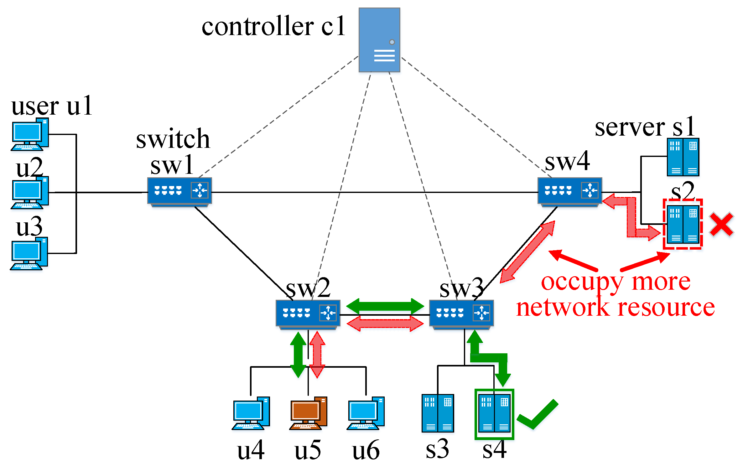
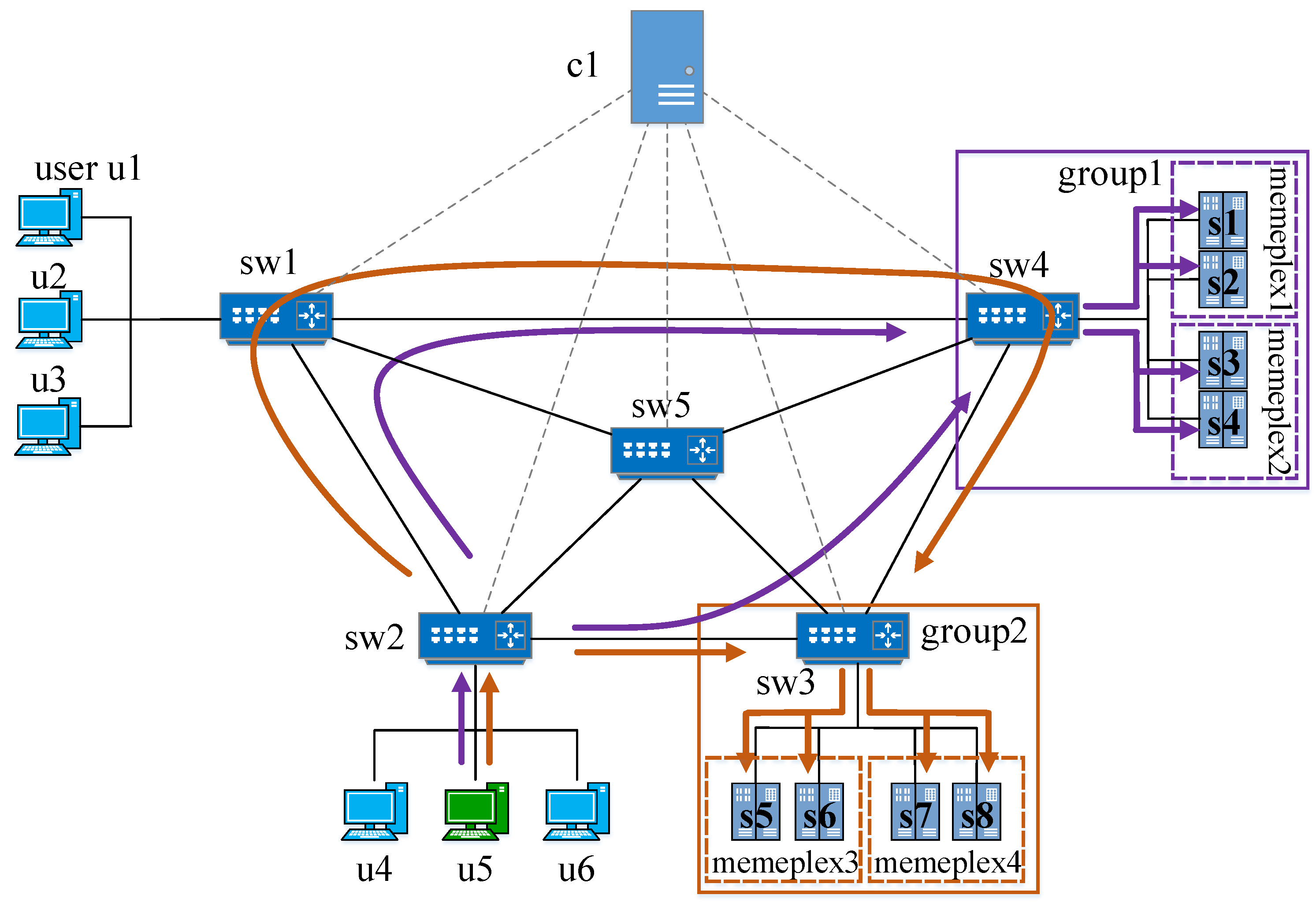
An example of that shortcoming is shown in Figure 1. In that figure, the servers s1, s2, s3 and s4 form a server cluster and provide the same service for the users u1, u2, u3, u4, u5 and u6. In that example, the user u5 tries to access the service provided by that server cluster. Assuming that the resource utilizations of s1, s2, s3 and s4 are 25 percent, 21 percent, 26 percent and 22 percent and the weighted least connection algorithm-based server load balancing method is employed, in the sequential server and routing path calculation, s2 will be firstly chosen as the destination server because that server is serving the least number of active sessions. Subsequently, the routing path u5-sw2-sw3-sw4-s2 will be established to carry the traffic between s2 and u5. Nevertheless, in this example, considering that the resource utilizations of s2 and s4 are very close, choosing s2 or s4 as the destination server has almost the same impact on the server load balancing. However, when selecting s4 as the destination server, the optimal routing path is u5-sw2-sw3-s4, which clearly occupies less network resource than the routing path u5-sw2-sw3-sw4-s2. In a word, the sequential destination server and routing path calculation method may affect the efficiency of the network. That is caused by the fact that the destination server calculation is carried out without considering its effect on the routing path. Thus, the destination server calculation often makes the routing path calculation unable to achieve a global optimal result.

Figure 1. Example of the shortcoming caused by sequential server selection and routing path calculation.

To address these shortcomings, we first propose the joint server selection and traffic routing problem in SDDC. Then, a Joint Server Selection and Traffic Routing algorithm (JSSTR) is designed to solve that problem based on the Shuffled Frog-Leaping Algorithm (SFLA) [12]. The main contributions of the paper are summarized below.

• The joint server selection and traffic routing problem is proposed and formulated.
• A joint server selection and traffic routing algorithm is presented to solve that problem, which is designed based on the SFLA algorithm.
• Several metrics are proposed and used to evaluate the performance on the routing path length, network load, network load balancing, server load, server load balancing and computational complexity of the proposed and compared algorithms.
• The proposed JSSTR algorithm and two compared algorithms are implemented and evaluated in SDN. The effectiveness of the proposed algorithm was proven using the above performance metrics.

This paper is organized as follows: Section 2 gives the description of the background. Section 3 lists and discusses the related work. Section 4 describes the system model and problem. The proposed algorithm and its implementation are illustrated in Section 5. The evaluation results are presented in Section 6 followed by the conclusions in Section 7.

2. Background

2.1. SFLA

SFLA is a meta-heuristic algorithm, which performs a heuristic search to solve the combinatorial optimization problem [12]. In SFLA, the possible solutions are recognized as frogs. At first, some frogs will be randomly generated as a sampled population. For each frog, a predefined performance value is computed. Then, these frogs are divided into several different communities (named memeplexes in SFLA). Each memeplex independently evolves to search the solution space in different directions. After a certain amount of evolutions, the memeplexes are mixed to form a new population. Subsequently, all frogs in that mixed population are re-divided into new memeplexes. Using these periodical shuffling, dividing and evolving processes, SFLA can converge to a global optimal solution with high probability [12]. More specifically, the main steps of SFLA are summarized below.

• Initialization: $\alpha$ and $\beta$ are firstly initialized. $\alpha$ represents the number of memeplexes. $\beta$ is the number of frogs in each memeplex.
• Generate a population: F frogs will be generated to form a population, where $F=\alpha \ast \beta$.
• Compute the performance value: For each frog, a performance value is firstly computed.
• Divide all frogs into $\alpha$ memeplexes. In this step, all frogs are divided into $\alpha$ memeplexes one by one in order of decreasing performance value.
• Evolution within each memeplex: Each memeplex is evolved according to the predefined local searching strategy.
• Shuffle memeplexes: After executing a certain number of evolutions, all frogs will be mixed. The performance values of all frogs will be computed again.
• Check convergence: If the convergence criteria are satisfied, SFLA will stop. Otherwise, it will return to Step 4.

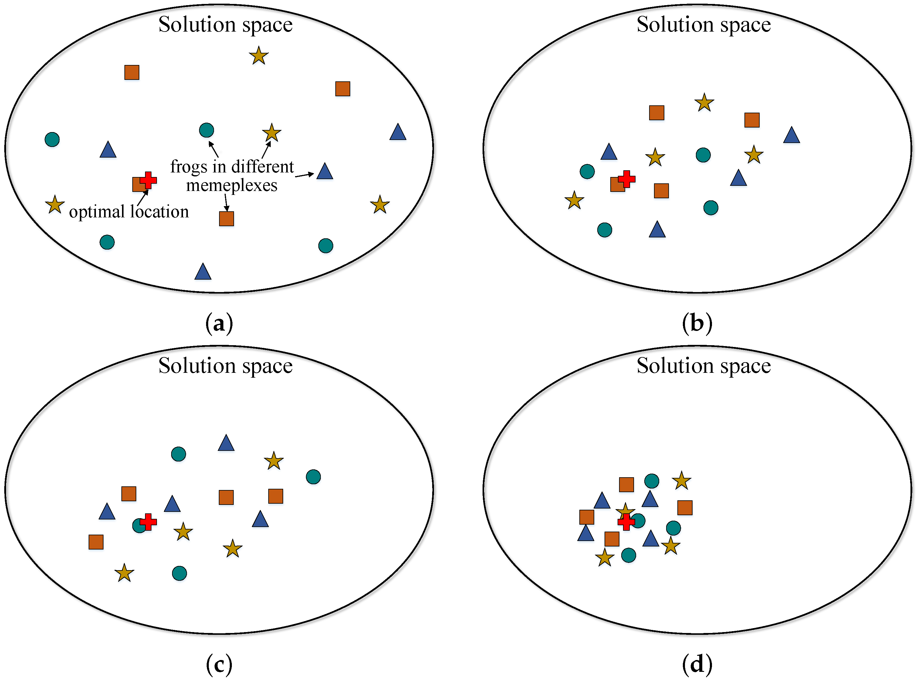
An example of SFLA is illustrated in Figure 2. In Figure 2a, 16 frogs are generated at the beginning of Time Loop 1. Then, these frogs are divided into four memeplexes, which are denoted by a triangle, square, pentagon and circle. After that, each memeplex independently executes a certain number of evolutions. Figure 2b shows the evolution result at the end of Time Loop 1. Subsequently, as shown in Figure 2c, in the next time loop, these frogs are mixed and re-divided into four new memeplexes. Again, each memeplex is independently evolved. Figure 2d shows the evolution result at the end of Time Loop 2. In Figure 2d, all frogs are clustering near the optimal location (denoted by a cross). The shuffling, dividing and evolving process will be periodically executed until the convergence criteria are satisfied.

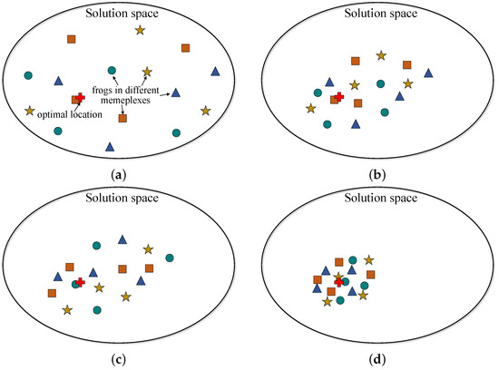
Figure 2. Illustration of SFLA. (a) At the beginning of Time Loop 1, 16 frogs are randomly generated and divided into four memeplexes (denoted by triangle, square, pentagon, and circle); (b) at the end of Time Loop 1, each memeplex is evolved; (c) at the beginning of Time Loop 2, all frogs are mixed and re-divided; (d) at the end of Time Loop 2, each memeplex is evolved.

3. Related Work

In a traditional network, the server load balancing technology has some shortcomings (e.g., inflexibility of updating and high cost). However, as a different network architecture, SDN provides new solutions to many issues. Meanwhile, SDN has already been widely accepted as the next generation of network in academia and industry, which means that the server load balancing technology should be applied in SDN and re-designed using new technology provided by SDN. However, currently, only a few works have been done to research how to achieve server load balancing in SDN.

An efficient SDN load balancing scheme was presented by Zhong et al. [11]. The key idea of that proposed scheme was distributing requests to different servers based on the response time of each server. More specifically, in that scheme, the controller periodically sends the packet-out messages to the switches. Then, the switches parse these packet-out messages and send the encapsulated requests to each server. Once the response is sent from the server, the switch will package that response into a packet-in message and send that packet-in message to the controller. After the controller receives that packet-in message, it will calculate the corresponding server’s response time. Once all servers’ response times are found, the controller will select the destination server using the following strategy. First, the maximum response time and minimum response time will be found and recorded as $T_{max}$ and $T_{min}$. Subsequently, if |$T_{max}-T_{min}$| < $\lambda$ (a predefined parameter), the server with the minimum response time will be chosen as the destination server. Otherwise, the server with the minimum standard deviation in m historical data of response time will be chosen as the destination server. Compared with other approaches, this method uses the SDN controller to measure the server response time instead of adding extra devices to realize that.

Chen et al. proposed a server load balancing algorithm used in SDN [13,14]. The proposed server load balancing algorithm first dynamically obtains the current load (CPU occupancy rate, memory occupancy rate and response time) of each server. Subsequently, the computation ability of each server will also be calculated. After that, the selection probability of each server will be calculated. At last, the server load balancing algorithm selects a server as the destination server based on that probability. Once the destination server has been chosen, related flow entries will be added in the OpenFlow switches [15,16]. Then, the subsequent user traffic will be sent to the chosen destination server.

A new probabilistic-based server load balancing method was proposed based on variance analysis by Zhong [17]. In that method, the SDN controller monitors the data traffic of each port, and the variance analysis is executed to analyze this traffic. Based on the analysis result, a probability-based selection algorithm is proposed to redirect the traffic dynamically. Using the Network Address Translation (NAT) technology, the presented server load balancing method can be implemented in SDN.

The performance of several SDN load balancing methods was evaluated by Silva [18]. The authors developed a comprehensive methodology for evaluating the SDN load balancers. The main steps of that methodology include the problem description, goals’ definition, metrics’ definition, evaluation techniques’ definition, architecture definition, hypothesis definition, workloads’ execution, results’ analysis and results’ presentation. Based on that methodology, the round-robin-, random- and CPU-usage based server load balancing strategies have been implemented and evaluated in SDN. The evaluation results show that these three algorithms achieve almost the same performance in the real scenario. However, in the virtual scenario, the CPU usage method performed better than the round-robin and random methods. Furthermore, the authors also evaluated the active load balancers and reactive load balancers in the SDN scenario. They found that the active load balancer performs better than the reactive load balancer.

Kaur et al. implemented the round-robin-based server load balancing strategy and compared that server load balancing strategy with the random-based server load balancing strategy in SDN [10]. These two load balancing strategies were implemented on the POXcontroller [19], and the evaluation results indicated that the round-robin-based server load balancing strategy works better than the random-based server load balancing strategy.

Besides that, the round-robin-based server load balancing strategy and least-connections-based server load balancing strategy were also implemented and compared in SDN [20]. Using Mininet [21,22] and Floodlight [23], the authors evaluated these two server load balancing strategies and found that the least-connections-based server load balancing strategy performs better than the round-robin-based server load balancing strategy.

Some server load balancing methods were also proposed for traditional networks. However, these load balancing methods can also be used in SDN. Chen et al. proposed a dynamic server load balancing method [24]. That method periodically obtains each server’s load and computes its priority value. When handling a user request, the first half of servers will be calculated in order of decreasing priority values. Then, a polling method is used to dispatch the request to these servers.

By classifying requests into different kinds, Sharifian et al. proposed a server load balancing algorithm to dynamically assign a request to a server [25]. In that algorithm, the Baskett, Chandy, Muntz and Palacios (BCMP) [26] and three approaches were employed to predict the server load. When selecting a destination server, the server with more available process-capacity has more chance of being selected.

Although the server load balancing technology plays an important role in networking, the SDN-based server load balancing technology has not caught so much attention. In contrast, as another key technology, the routing technology has been widely studied in SDN. Many routing methods used in SDN have been proposed.

The authors in [27] proposed a unicast routing algorithm based on the Bellman–Ford algorithm. In that algorithm, the first k shortest paths between every possible pair are computed and used to calculate the defined criticality of each link. The amount of traffic flows and remaining bandwidth of each link are utilized to find the congestion index. The above criticality and congestion index compose the link weight. At last, the Bellman–Ford algorithm with a hop count constraint is executed to calculate the routing path between the source and destination. The link’s residual bandwidth, path length and link criticality are considered in this work.

In [28], an application-aware routing algorithm was proposed. That routing algorithm allocates paths for the incoming requests in batches. When allocating paths, it first sorts the incoming requests. Subsequently, for each request, if it is a pod-local request, the only available path inside that pod is used as the routing path. Otherwise, the current link loads, and the recorded bandwidth usages of every pod are checked to calculate a best path for that request.

The authors in [29] proposed an adaptive routing algorithm with QoS support in SDN. In their algorithm, the video packets are classified into base layer packets and enhancement layer packets. When the controller receives the video packets for the first time, the Dijkstra algorithm is employed to calculate the shortest routing path between the source and destination. Once that path does not satisfy the delay constraint, the base layer packets will be rerouted to another feasible path, and the enhancement layer packets still stay on the original path. Nevertheless, if the path does not have enough available bandwidth, the enhancement layer packets will be rerouted while the base layer packets stay on the original path.

In [30], a method about how to implement a reinforcement learning-based routing protocol in the SDN was proposed. The method first calculates a set of possible routing paths based on the delay, loss rate and bandwidth of network devices. Then, different weights are assigned to these parameters. Afterwards, the path that has the least cost is chosen as the routing path to transfer the corresponding traffic. After some time, the routing path gives feedback to the controller. After receiving that feedback, the controller adjusts the weights of these network parameters and tries to find a better routing path. Results show that the proposed routing method works properly and satisfies the QoS constraint preferably.

In [31], the authors proposed a bandwidth-delay-constrained routing algorithm. The authors classified the requests into two kinds including the one that is delay-sensitive and another one that is not delay-sensitive. The proposed algorithm contains two phases: the offline phase and online phase. In the offline phase, the first k shortest paths are calculated for each source-destination pair using Yen’s algorithm. In the online phase, if the request belongs to delay-sensitive requests, the path with least weight is chosen from the set of paths that are calculated in the offline phase. Otherwise, the Dijkstra algorithm is employed to find a shortest routing path.

In [32], the QoS-aware resource reallocation problem that considers traffic prediction in SDN was formulated, which belongs to binary linear programming. In order to solve that problem with less computational complexity, the authors relaxed the objective function by forwarding table entries and proposing an upper bound function for the objective function. The Convex Programming Language (CVX) toolbox of MATLAB was used to solve that problem. The evaluation results demonstrated the effectiveness of the proposed algorithm.

The authors in [33] proposed a routing model used in SDN. In their model, for each pair of switches, the routing path between these two switches is firstly calculated. When the controller receives a request, it will find the switches that connect to the source and destination host of that request. Then, the hash-based modulo assignment operation is performed to determine which path should be assigned to that request. Afterwards, the routing path is established to transfer traffic generated by the request.

The main differences between the proposed method in this paper and the exiting methods are listed in Table 1. Unlike the existing methods, the proposed method introduces and formulates the joint server selection and traffic routing problem, which belongs to the NP-hard problems. In order to solve that problem, a meta-heuristic algorithm (JSSTR), which is designed based on the SFLA algorithm, was proposed. Evaluation results showed that the proposed JSSTR algorithm can achieve high network utilization, network load balancing and server load balancing simultaneously.

Table 1. Main differences between the proposed method and the exiting methods. BCMP, Baskett, Chandy, Muntz and Palacios.

No.	Authors	Technique	Research Focus/Contribution/Features
1	Zhong et al. [11]	Controller-based server response time measurement; Dynamic server selection	The controller periodically sends packet-out messages to measure server response time. There is no need to add extra devices to measure server response time. The server with the minimum response time or minimum standard deviation in m historical data of response time will be chosen as the destination server based on the difference value between maximum and minimum server response time.
2	Chen et al. [13,14]	Dynamic feedback of server load; Probability-based server selection	The CPU occupancy rate, memory occupancy rate and response time are collected and recorded as the server load. The weight and selection probability of all servers will be calculated as the servers’ load change. The system selects a server as the destination server based on the calculated selection probability.
3	Zhong et al. [17]	Variance analysis; Probability-based server selection; Network address translation	The F-test method is executed to analyze the data traffic of each port. The selection probability of each port is calculated. The traffic is dynamically redirected based on the selection probability.
4	Silva et al. [18]	Evaluating the SDN load balancers; round-robin; random; CPU usage	A comprehensive methodology for evaluating the SDN load balancers is proposed. The performance of the round-robin-, random- and CPU usage-based server load balancing strategies is evaluated. The active and reactive load balancers are evaluated in the SDN scenario.
5	Kaur et al. [10]	Round-robin-based load balancing method; Random-based load balancing method	The round-robin- and random-based server load balancing method are implemented and evaluated. The evaluation results indicate that the round-robin-based load balancing method works better than the random-based method.
6	Zhang et al. [20]	Round-robin-based server load balancing method; Least-connections-based server load balancing method	The round-robin-based server load balancing method and least-connections-based server load balancing method are implemented and compared in SDN. It is found that the least-connections-based server load balancing method performs better than the round-robin-based server load balancing method.
7	Chen et al. [24]	Dynamic server load balancing; Priority-based server selection; Polling method	The proposed dynamic server load balancing method periodically obtains each server’s load and computes its priority value. The first half of servers will be listed in order of decreasing priority values. A polling method is used to dispatch requests to these servers.
8	Sharifian et al. [25]	Predicting the server load; Classifying user requests; BCMP queuing model	The user requests are classified into dynamic and static requests. The BCMP queuing network model is designed to estimate the resource utilization and average response time of the web server. The utility function, RBF neural networks and adaptive neuron-fuzzy inference system are proposed to adjust the predicted values of the queuing model.
9	Lee et al. [27]	Bellman–Ford algorithm; Self-defined criticality and congestion index of link	It computes and uses the first k shortest paths between every possible pair to calculate the defined criticality of each link. The amount of traffic flows and remaining bandwidth of each link are utilized to find the congestion index. The Bellman–Ford algorithm is executed to calculate the routing path between the source and destination.
10	Cheng et al. [28]	Application-aware routing; Process requests in batches	An application-aware SDN routing scheme for Hadoop MapReduce processing is proposed. It allocates paths for the incoming requests in batches. It outperforms the ECMP-RRscheme, spanning tree scheme and the Floodlight OpenFlow controller.
11	Yu et al. [29]	Dijkstra algorithm; Rerouting; Classifying packets into two kinds	Base layer packets and enhancement layer packets are treated separately as two levels of QoS flows. It reroutes the base layer packets or the enhancement layer packets based on the network status.
12	Sendra et al. [30]	Reinforcement learning-based routing; Feedback-based weight adjusting	A reinforcement learning method is proposed to establish a path between the source and destination. The weights of different parameters (delay, loss rate and band-width) are recalculated according to the feedback. Evaluation results show that it works properly and reaches better QoS features than the traditional OSPFrouting protocol.
13	Tomovic et al. [31]	Bandwidth-delay-constrained routing; Yen’s algorithm; Offline and online phase	It can calculate the routing path with the bandwidth-delay constraint. The offline phase and online phase are designed to quickly handle user requests.
14	Tajiki et al. [32]	QoS-aware; Binary linear programming; Relaxing objective function	It supports different traffic classes with various QoS requirements. It makes a trade-off between performance and computational complexity.
15	Celenlioglu et al. [33]	Pre-establishing paths; Hash-based modulo assignment operation	It can effectively make the routing path and manage the network resource. Multi-paths are pre-established in offline mode to prevent the controller from becoming a bottleneck. It performs adaptive load balancing by equalizing path costs.
16	This paper	Joint server selection and traffic routing; Combinatorial optimization problem; SFLA algorithm	The joint server selection and traffic routing problem is proposed and formulated. A joint server selection and traffic routing algorithm is presented, which is designed based on the SFLA algorithm. Several metrics are proposed and used to evaluate the proposed algorithm.

4. System Model and Problem Statement

4.1. The SDDC Model

Assume that the SDDC network $G=(V,E,S)$ contains switches denoted by $V=\{v_1,v_2,\dots ,v_n\}$ and servers denoted by $S=\{s_1,s_2,\dots ,s_m\}$. Servers and switches are connected by links $E=\{e_{i,j}=(i,j)|i,j\in \{V,S\}andi\ne j\}$. The detailed description of notations used in this work is shown in the Abbreviations part of this paper.

For a request, the total link cost of its routing path p is defined as ${\displaystyle \sum _{e_{i,j}\in p}}{c}_{i,j}$. Here, $c_{i,j}$ is the cost of allocating the k-th request on the link $e_{i,j}$, and it is calculated by $c_{i,j}=u_{i,j}\ast b_k$, where $u_{i,j}$ is the unit cost of link $e_{i,j}$ and $b_k$ is the bandwidth required by the request. At the same time, the bandwidth utilization ratio of link $e_{i,j}$ is expressed as $l_{i,j}$. It is denoted by $l_{i,j}=u{b}_{i,j}/t{b}_{i,j}$, where $u{b}_{i,j}$ and $t{b}_{i,j}$ represent the occupied bandwidth and total bandwidth of link $e_{i,j}$, respectively. Thus, for a request, the bandwidth utilization ratio of its routing path p is defined as ${\displaystyle \sum _{e_{i,j}\in p}}{l}_{i,j}$.

Likewise, the resource utilization ratio of a server is defined as the percentage between the used resource (CPU, memory and disk) and total resource of the server. Therefore, the resource utilization ratio of server $s_i$ is expressed as $l_i={\delta }_c\ast l{c}_i+{\delta }_m\ast l{m}_i+{\delta }_d\ast l{d}_i$. The $l{c}_i$, $l{m}_i$ and $l{d}_i$ are the CPU utilization ratio, memory utilization ratio and disk utilization ratio, respectively. For instance, the memory utilization ratio is calculated by $l{m}_i=u{m}_i/t{m}_i$, where $u{m}_i$ and $t{m}_i$ refer to the used memory and total memory of the server. Meanwhile, ${\delta }_c$, ${\delta }_m$ and ${\delta }_d$ are the coefficients of CPU, memory and disk resource, respectively. In this work, we focus on how to design a meta-heuristic algorithm to solve the joint server selection and traffic routing problem. We did not give much attention to assigning these parameters. Therefore, these parameters are constant, and the ${\delta }_c$, ${\delta }_m$ and ${\delta }_d$ are all set to 1/3.

4.2. Joint Server Selection and Traffic Routing Problem

The joint server selection and traffic routing problem is described and formulated in this section. In that problem, the traffic refers to the data transmission between the user and the destination server. To make the calculated routing path have a low cost while the network and server load balancing are realized, the fitness of the server and routing path is defined as $sf=l_i$ and $pf={\displaystyle \sum _{e_{i,j}\in E}}(c_{i,j}+l_{i,j})$. Then, the joint server selection and traffic routing problem can be formulated as follows.

Minimize:

$${\displaystyle \sum _{e_{i,j}\in E}}{x}_{i,j}\ast (c_{i,j}+l_{i,j})+{\displaystyle \sum _{s_i\in S}}{y}_i\ast l_i$$

(1)

Subject to:

$$t{b}_{i,j}-u{b}_{i,j}\ge b_k$$

(2)

$$t{r}_i-u{r}_i\ge r_k$$

(3)

$${\displaystyle \sum _{y_i\in S}}{y}_i\le 1$$

(4)

$$x_{i,j},y_i\in \{0,1\}$$

(5)

$x_{i,j}$ is defined to indicate whether the link $e_{i,j}$ is chosen as the routing path, and $y_i$ represents whether the server $s_i$ is chosen as the destination server. Equations (2) and (3) ensure that the remaining resource of the chosen routing path and destination server is enough for the request. Equation (4) guarantees that the request will be responded to by at most one server. Equation (5) indicates that a link or a server will either be chosen or not.

Essentially, the routing path calculation problem in the joint server selection and traffic routing problem belong to the Multi-Commodity Flow (MCF) problem, which is a well-known NP-hard problem. However, the joint server selection and traffic routing problem is more complex than the MCF problem as it needs to choose one server from a number of servers. Moreover, the joint server selection and traffic routing problem is also a combinatorial optimization problem, which makes it even harder. In conclusion, the joint server selection and traffic routing problem belongs to the NP-hard problems, which means that there is no polynomial-time solutions for it. Therefore, in the next session, a heuristic method is designed to find the approximate optimal solution of the joint server selection and traffic routing problem in polynomial time.

5. Joint Server Selection and Traffic Routing Algorithm

5.1. Design Principle

As explained before, the joint server selection and traffic routing problem belongs to the NP-hard problems. Hence, by improving the SFLA, a heuristic algorithm is developed to solve the joint server selection and traffic routing problem. The proposed JSSTR algorithm is designed based on the improved SFLA. Unlike the original SFLA, the improved SFLA contains two kinds of frogs, one population, several groups and several memeplexes. The definitions of the two kinds of frogs, population, group and memeplex are given as follows.

• server frog: In the proposed JSSTR algorithm, the switch that connects to servers is called the edge switch. Based on that, two kinds of frogs are defined and used in JSSTR: server frog and switch frog. A server frog is composed of the user, the destination server and the routing path between that user and server.
• switch frog: A switch frog is composed of the user, the corresponding edge switch and the routing path between the user and the edge switch.
• population: All server frogs form a population.
• group: A group is generated for each edge switch. All server frogs, the destination servers of which connect to the same edge switch, are recorded as a group.
• memeplex: All server frogs in a group are divided into several memeplexes.

As mentioned in Section 2, two of the main steps of SFLA are shuffling and dividing memeplexes. In the original SFLA algorithm, when dividing frogs into different memeplexes, a performance value of each frog will be calculated. Then all frogs will be divided into several memeplexes one by one in order of decreasing performance value.

Note that a user request causes different workloads on the network and server. It mainly uses the bandwidth resource of links, while it uses CPU, memory and disk resource of servers. Therefore, when serving a user request, the changes of the performance value of links and servers are different. Meanwhile, in the joint server selection and traffic routing problem, a server frog is composed of the routing path and server. Hence, in the same group, if a server frog has the best performance value, the routing path and server of that server frog should have the best performance value.

Therefore, in this work, in order to more quickly find the server frog that has the best performance value, we designed two kinds of frogs: (1) server frog and (2) switch frog. These two frogs are used in shuffling and dividing the steps of SFLA. Taking advantage of the switch frog, the proposed JSSTR method will more quickly find an optimal server frog using the following strategy. When shuffling memeplexes, the switch frogsare firstly extracted from the server frogs. Then, the performance value of all switch frogs are calculated. Subsequently, these switch frogs are mixed and re-divided into several memeplexes one by one in order of decreasing performance value. Afterwards, the server and the link between that server and the corresponding edge switch are added to each switch frog in order of decreasing performance value to form the new server frogs.

An example of that is given in this paragraph. In Figure 3, assume that four server frogs of Group 2 are server frog 1: u5-sw2-sw3-s5, server frog 2: u5-sw2-sw5-sw3-s6, server frog 3: u5-sw2-sw3-s7, and server frog 4: u5-sw2-sw1-sw4-sw3-s8. According to its definition, the corresponding switch frogs extracted from these four server frogsare switch frog 1: u5-sw2-sw3, switch frog 2: u5-sw2-sw5-sw3, switch frog 3: u5-sw2-sw3 and switch frog 4: u5-sw2-sw1-sw4-sw3.

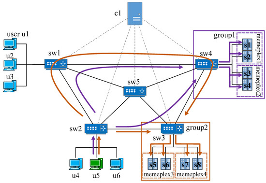
Figure 3. Design principle of the JSSTR algorithm.

Consider such a scenario: before shuffling and dividing frogs, the server frog 2 has the maximum performance value, while switch frog 1 and switch frog 4 (u5-sw2-sw3) have the maximum performance value and the server $s6$ and its connected link have the maximum performance value. That scenario is possible because the performance values of links and servers are independent, as discussed above. In that case, taking advantage of the switch frog and the shuffling and dividing strategy mentioned above, it is easy to find a new server frog: u5-sw2-sw3-s6, which has obviously a bigger performance value than the original server frog 2.

The JSSTR algorithm executes several time loops. At the beginning of the first time loop, the server frogs are firstly initialized using the following strategy. First, the edge switches that connect to the servers that can provide service for the user request are found. Then, the Depth First Search (DFS) algorithm is used to calculate a number of routing paths between the user and these edge switches. Each routing path and the user form a switch frog. After all switch frogs are generated, for each edge switch in the edge switches, its connected servers that can provide service for the user request are calculated. Then, these servers and the corresponding links between these servers and the edge switch are added to the switch frogs to form the server frogs.

After all server frogs are initialized, the server frogs in the same group are divided into several memeplexes. Each memeplex executes a certain number of evolutions independently at the end of the first time loop. In the next time loop, the server frogs in the same group are mixed and re-divided into new memeplexes using the shuffling and dividing method mentioned above. Then, these server frogs evolve at the end of this time loop. The time loop will not stop until the number of time loops reaches the maximum number or the difference between the performance values of the current best frog and the last best frog reaches the prespecified value.

An example of the proposed JSSTR algorithm is illustrated in Figure 3 and Table 2. In Table 2, $f1,f2,f3,f4,f5,f6,f7$ and $f8$ are server frogs. At first, these eight server frogs are initialized as the population, as shown in Table 2. There are two edge switches in Figure 3. Accordingly, two groups (i.e., Group 1 and Group 2) are formed by corresponding server frogs. At the beginning of Time Loop 1, in each group, all server frogs are divided into two memeplexes, such as Memeplex 3 and Memeplex 4 in Group 2. At the end of Time Loop 1, each memeplex evolves independently. For example, $f6$ evolves from u5-sw2-sw1-sw4-sw3-s6 to u5-sw2-sw5-sw3-s6. Then, in Group 1 and Group 2, the switch frogs are extracted from server frogs. Take Group 2 as an example: at the end of Time Loop 1, the server frogs after evolution are u5-sw2-sw3-s5, u5-sw2-sw5-sw3-s6, u5-sw2-sw1-sw4-sw3-s7 and u5-sw2-sw3-s8, and the corresponding switch frogs extracted from these server frogs are u5-sw2-sw3, u5-sw2-sw5-sw3, u5-sw2-sw1-sw4-sw3 and u5-sw2-sw3. These switch frogs, listed in order of decreasing performance value, are u5-sw2-sw3, u5-sw2-sw3, u5-sw2-sw5-sw3 and u5-sw2-sw1-sw4-sw3. Also listed in order of decreasing performance value, the servers and paths between the server and sw3 are -s5, -s7, -s6 and -s8. Therefore, the new server frogs, which are re-divided into Memeplex 3, are u5-sw2-sw3-s5 and u5-sw2-sw5-sw3-s6, while the server frogs in Memeplex 4 are u5-sw2-sw3-s7 and u5-sw2-sw1-sw4-sw3-s8. Then, the new memeplexes evolve independently. At last, if the convergence criteria are satisfied, the JSSTR stops. The server frogs in the final time loop are shown in Table 2. In that case, the server frog $f5$ will be chosen as the final solution as it has the best performance value.

Table 2. Example of JSSTR.

Time Loop	Group 1		Group 2
	Memeplex 1	Memeplex 2	Memeplex 3	Memeplex 4
begin of time loop 1	$f1$: u5-sw2-sw3-sw4-s1; $f2$: u5-sw2-sw1-sw4-s2;	$f3$: u5-sw2-sw3-sw4-s3; $f4$: u5-sw2-sw1-sw4-s4;	$f5$: u5-sw2-sw3-s5; $f6$: u5-sw2-sw1-sw4-sw3-s6;	$f7$: u5-sw2-sw3-s7; $f8$: u5-sw2-sw1-sw4-sw3-s8;
end of time loop 1	$f1$: u5-sw2-sw1-sw4-s1; $f2$: u5-sw2-sw3-sw4-s2;	$f3$: u5-sw2-sw3-sw4-s3; $f4$: u5-sw2-sw1-sw4-s4;	$f5$: u5-sw2-sw3-s5; $f6$: u5-sw2-sw5-sw3-s6;	$f7$: u5-sw2-sw1-sw4-sw3-s7; $f8$: u5-sw2-sw3-s8;
begin of time loop 2	$f1$: u5-sw2-sw1-sw4-s1; $f2$: u5-sw2-sw3-sw4-s2;	$f3$: u5-sw2-sw1-sw4-s3; $f4$: u5-sw2-sw3-sw4-s4;	$f5$: u5-sw2-sw3-s5; $f6$: u5-sw2-sw5-sw3-s6;	$f7$: u5-sw2-sw3-s7; $f8$: u5-sw2-sw5-sw4-sw3-s8;
end of time loop 2	$f1$: u5-sw2-sw1-sw4-s1; $f2$: u5-sw2-sw3-sw4-s2;	$f3$: u5-sw2-sw1-sw4-s3; $f4$: u5-sw2-sw5-sw4-s4;	$f5$: u5-sw2-sw3-s5; $f6$: u5-sw2-sw5-sw3-s6;	$f7$: u5-sw2-sw3-s7; $f8$: u5-sw2-sw5-sw3-s8;
...
final time loop	$f1$: u5-sw2-sw1-sw4-s1; $f2$: u5-sw2-sw1-sw4-s2;	$f3$: u5-sw2-sw1-sw4-s3; $f4$: u5-sw2-sw5-sw4-s4;	$f5$: u5-sw2-sw3-s5; $f6$: u5-sw2-sw3-s6;	$f7$: u5-sw2-sw3-s7; $f8$: u5-sw2-sw3-s8;

5.2. Detailed Description of JSSTR

As shown in Algorithm 1, for solving the above joint server selection and traffic routing problem, an algorithm called JSSTR is proposed based on SFLA. When the controller receives a request sent from the user, it will first parse that request to get its source IP address $src\_ip$, destination IP address $dst\_ip$ and protocol type $pro\_type$. Then, $u{b}_{i,j}$, $t{b}_{i,j}$ of all links and $u{r}_i$ and $t{r}_i$ of all servers are obtained. All servers that can provide service for the user request and all edge switches that connect to those servers are calculated based on the $dst\_ip$.

From Line 5–Line 8, for each switch in all edge switches $e\_switches$, JSSTR firstly calculates m initial routing paths between that switch and the user by using the DFS algorithm. The user and a routing path of the initial routing paths form a switch frog. After that, one server is randomly chosen from the servers that connect to that switch. Then, the corresponding server frog will be generated by that chosen server, the link between the chosen server and the switch and the switch frog. Accordingly, all switch frogs and server frogs are generated in that way. The server frogs that have the same edge switch form a group, each for an edge switch.

From Line 9–Line 16, JSSTR carries out several time loops. In each time loop, all server frogs are firstly divided into a number of memeplexes using the function $divide\_frogs$. Then, each memeplex executes a certain number of local optimizations. Subsequently, the maximum fitness of all server frogs is calculated in function $calc\_maximum\_fitness$ by using $fitness=1/(1+pf+sf)$, where $pf$ and $sf$ are defined in Section 4.2. The difference value $maximum\_fitness\_diff$ of the current maximum fitness $maximum\_fitness$ and the maximum fitness of the last time loop $last\_maximum\_fitness$ is calculated. If the number of the time loops reaches the maximum number $maximum\_time\_loop\_num$ or the difference value $maximum\_fitness\_diff$ reaches the threshold value $fitness\_diff\_threshold$, the time loop will stop. Afterwards, the server frog that has maximum fitness is found. The server and path of that server frog are chosen as the destination server $s_d$ and routing path $p_r$. At last, some flow entries are installed on the switches based on $s_d$ and $p_r$ (Line 18).

The function $divide\_frogs$ is used to divide all server frogs into n memeplexes for each group. In that function, for each $e\_switch$ in $e\_switches$, all switch frogs are firstly extracted by subtracting the destination server and the link that connects that server and the corresponding $e\_switch$ from the server frogs. Then, these switch frogs are sorted in order of decreasing fitness and stored in $ordered\_switch\_frogs$. Afterwards, all servers connected to that $e\_switch$ are found and recorded as $sw\_servers$. Simultaneously, the number of $sw\_servers$ is recorded as l. For all $sw\_servers$, the servers and the links connected to these $sw\_servers$ are sorted in order of decreasing fitness and recorded as $ordered\_servers\_links$. Then, for the i-th $sw\_frog$ in $ordered\_switch\_frogs$, the ($i\%l$)-th element of $ordered\_servers\_links$ is added to that $sw\_frog$ to form a new server frog. Meanwhile, the new generated server frog is divided to the ($i\%n$)-th memeplex.

The local evolution based on the Genetic Algorithm (GA) is carried out in function $local\_evolution$, from Line 36–Line 47. The main steps of local evolution are $calc\_fitness$, $cross\_frogs$, $remove\_loop$ and $mutate\_frogs$. In function $calc\_fitness$, each server frog’s fitness is calculated using $fitness=1/(1+pf+sf)$.

Function $cross\_frogs$ is designed to generate new server frogs to search the solution space more broadly. The elitist reserve and tournament selection strategy are employed to select server frogs, which can ensure that the server frogs with bigger fitness have more chance to survive. More specifically, the elitist reserve strategy is firstly used to select a server frog, which has maximum fitness, and reserve that server frog when crossing server frogs to ensure that the best server frog will not be broken. Then, the tournament selection is carried out $h-1$ times to choose $h-1$ server frogs, where h is the number of server frogs in that memeplex. After that, two server frogs (for example, $p_1$,$p_2$) that have at least one same node are selected at a probability $p_c$. Then, one of those same nodes will be randomly chosen as the location of crossover. At last, the two sub-paths of $p_1$ and $p_2$ after that node will be exchanged to form new server frogs $p_1^{\prime }$ and $p_2^{\prime }$.

The function $mutate\_frogs$ is used to enhance the local searching capability of JSSTR. In $mutate\_frogs$, a server frog is randomly selected with probability $p_m$. Afterwards, one node (except the last node and the node that is the previous hop of edge switch) of that server frog is randomly chosen as the mutating location. Then, the selected mutating node randomly chooses another node, which connects to it as its next hop. Meanwhile, the path between that chosen next hop and the end node is calculated using the DFS algorithm. Finally, the sub-path before the mutating node and the newly calculated path are combined to form a new server frog.

After crossing and mutating server frogs in a memeplex, there may be redundancy loops in new server frogs. Therefore, in order to remove the redundancy loops, the function $remove\_loop$ is designed to check the crossed and mutated server frogs and remove all redundancy loops. If the number of local evolution reaches the pre-defined maximum evolution number, the local evolution in the memeplex will stop.

Algorithm 1 JSSTR

Require:  $G=\{V,E,S\}$, request R, number of $server\_frogs$m of each group and number of memeplexes n of each group Ensure:  destination server $s_d$ and routing path $p_r$

1: $src\_ip,dst\_ip,pro\_type\leftarrow parse(R)$    2: For every link $e_{i,j}\in E$ and every server $s_i\in S$, get $u{b}_{i,j}$, $t{b}_{i,j}$, $u{r}_i$ and $t{r}_i$    3: $servers\leftarrow find\_dst\_servers(dst\_ip)$    4: $e\_switches\leftarrow find\_connect\_switch(servers)$    5: for$switch$ in $e\_switches$ do    6:     $switch\_frogs[switch.id]\leftarrow dfs(src\_ip,e\_switch)$    7:     $server\_frogs\leftarrow generate\_server\_frogs(switch\_frogs,switch)$    8: end for    9: $last\_maximum\_fitness\leftarrow 0$   10: while$(time\_loop\_num<maximum\_time\_loop\_num$and$maximum\_fitness\_diff<fitness\_diff\_threshold)$do   11:     $memeplexes\leftarrow divide\_frogs(server\_frogs,n)$   12:     $memeplexes\leftarrow local\_evolution(memeplexes)$   13:     $maximum\_fitness\leftarrow calc\_maximum\_fitness(memeplexes)$   14:     $maximum\_fitness\_diff\leftarrow abs(maximum\_fitness-last\_maximum\_fitness)$   15:     $last\_maximum\_fitness\leftarrow maximum\_fitness$   16: end while   17: $s_d,p_r\leftarrow find\_index(maximum\_fitness)$   18: Insert flow entries based on $s_d$ and $p_r$   19:     20: function$divide\_frogs$($server\_frogs$, n)   21:     for $e\_switch$ in $e\_switches$ do   22:         $i=0$   23:         $switch\_frogs\leftarrow extract\_server\_frogs(server\_frogs,switch)$   24:         $ordered\_switch\_frogs\leftarrow sort(switch\_frogs)$   25:         $l,sw\_servers\leftarrow find\_connect\_servers(switch)$   26:         $ordered\_servers\_links\leftarrow sort(sw\_servers+s\_links)$   27:         for $sw\_frog$ in $ordered\_switch\_frogs$ do   28:            $server\_frog\leftarrow sw\_frog+ordered\_servers\_links[i\%l]$   29:            $memeplexes[i\%n].append(server\_frog)$   30:            $i++$   31:         end for   32:     end for   33:     return $memeplexes$   34: end function   35:     36: function$local\_evolution$($memeplexes$)   37:     for $memeplex$ in $memeplexes$ do   38:         while $evolution\_num<maximum\_evolution\_num$ do   39:            $memeplex.fitness\leftarrow calc\_fitness(memeplex)$   40:            $memeplex\leftarrow cross\_frogs(memeplex)$   41:            $memeplex\leftarrow remove\_loop(memeplex)$   42:            $memeplex\leftarrow mutate\_frogs(memeplex)$   43:            $memeplex\leftarrow remove\_loop(memeplex)$   44:         end while   45:     end for   46:     return $memeplexes$   47: end function

5.3. Implementation

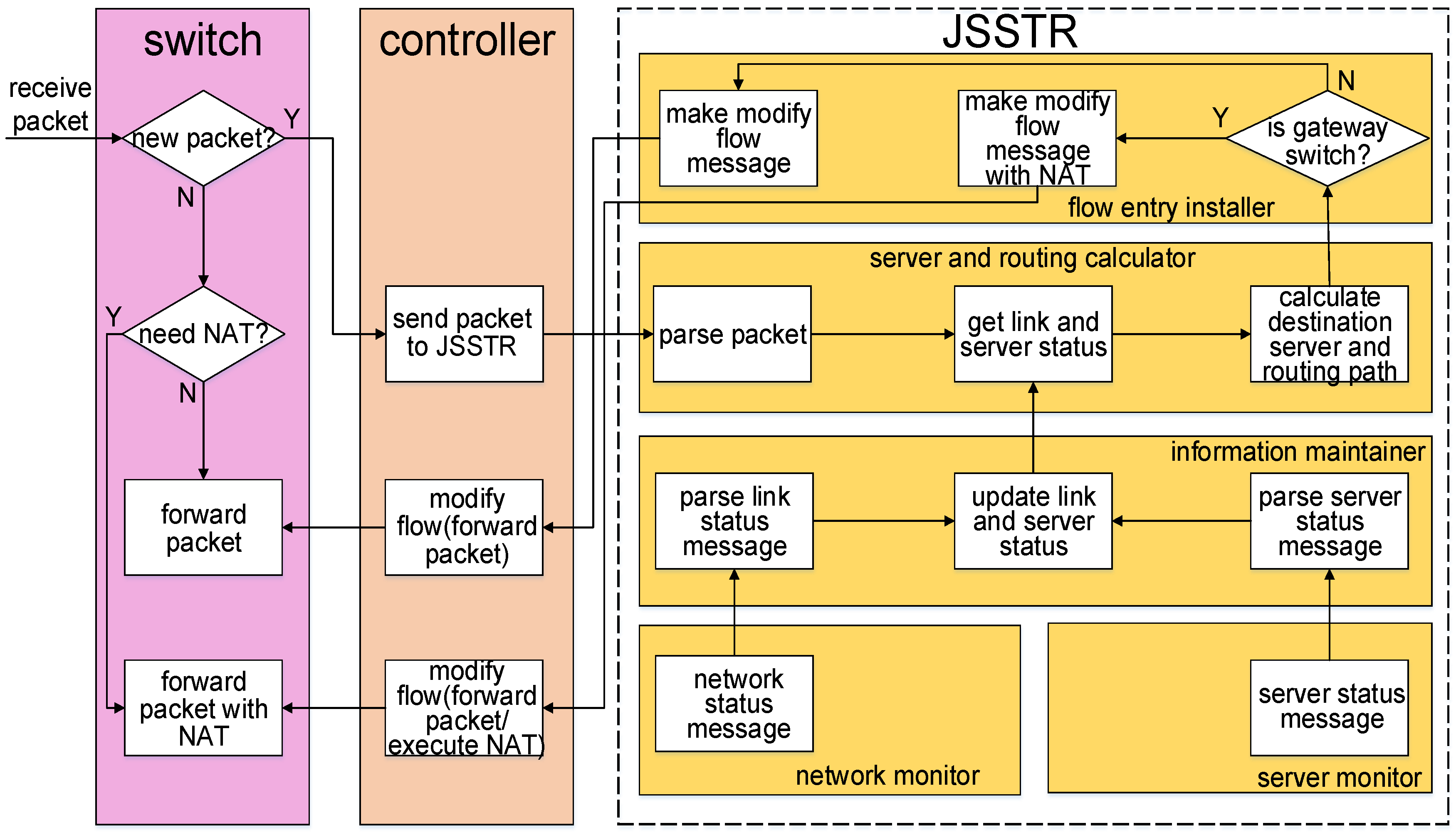
To validate our design, the proposed algorithm has been implemented as a module of the RYU controller. As shown in Figure 4, the implemented JSSTR is composed of the server and routing path calculator , flow entry installer, information maintainer, server monitor and network monitor. It should be noted that in Figure 4 , NAT is the abbreviation of Network Address Translation. When the OpenFlow switch receives a packet, the switch will find out whether there is a flow entry in the switch that can match that packet. If there is no matched flow entry, the packet will be sent to the SDN controller. After that, the server and routing path calculator firstly gets the information of the network devices and servers from the information maintainer. Using this information, the destination server and routing path are calculated by the JSSTR algorithm. Subsequently, the flow entry installer generates the corresponding forwarding rules and installs flow entries in the relevant switches. Finally, the traffic between the user and server will be transmitted by the established routing path, and the server will provide service for this user. The detailed description of the main components is given below.

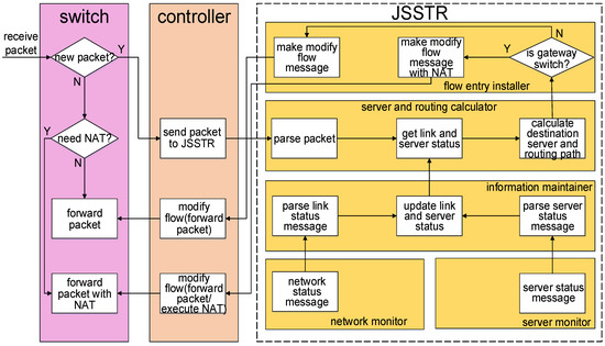
Figure 4. The implementation of the Joint Server Selection and Traffic Routing (JSSTR) algorithm.

Server and routing path calculator: The destination server and routing path calculation are implemented in this module. When the SDN controller receives a new packet, this packet will be firstly sent to this module. The relevant information (e.g., source IP address, destination IP address, protocol type of network layer, and so on) will be parsed from the packet. Afterwards, the detailed information of all links and servers will be obtained from the information maintainer. Then, the JSSTR algorithm implemented in the server and routing path calculator can calculate the destination server and routing path.

Flow entry installer: This module generates and installs forwarding rules for the processed packet based on the calculation result made by the server and routing path calculator. Basically, the main forwarding rules include forwarding packets to a specified port and executing the NAT strategy. For the switch that connects to users, the NAT strategy will be executed on the packets transmitted through it. More specifically, for packets sent from the user to the server, its source IP address and MAC address will be modified to the switch’s IP and MAC address. Meanwhile, its destination IP and MAC address will be modified to the destination server’s IP and MAC address. In contrast, for packets sent from the server to the user, the source IP and MAC address will be modified to the gateway’s IP and MAC address. In addition, the destination IP and MAC address will be modified to the user’s IP and MAC address. The NAT strategy is only executed in the switches that connect to users. For other switches, they just forward the arriving packets without modifying the IP or MAC address of these packets. Information maintainer: This module is responsible for storing the link and server information and providing this information to the server and routing path calculator. After receiving messages sent from the network monitor and server monitor, this module will parse these messages to get and store the bandwidth usage of the links and resource usage of the servers. When the server and routing path calculator needs the link and server information, the relevant information will be provided.

Server monitor: The server monitor is designed to collect the server information by the controller. In this work, a program written in Python is used to simulate and monitor the resource usage of these servers. In order to quickly respond to the user request, the server monitor periodically collects the CPU information, memory information and hard disk information and sends this information to the information maintainer. As previous work in [13], the periodic interval used in this work is set to 5 s.

Network monitor: By periodically sending the $ofp\_port\_stats\_request$ message (a special kind of OpenFlow message that is sent by the controller to get the port status of a switch), this module can monitor all links in the network. When a switch receives a $ofp\_port\_stats\_request$ message, it will send the $ofp\_port\_stats\_reply$ message back to this module. Then, this module will parse the $ofp\_port\_stats\_reply$ message and send the link information to the information maintainer. More specifically, this module uses the following method to measure the occupied bandwidth of each link. The received $ofp\_port\_stats\_reply$ is firstly parsed to get the switch ID, port number, number of received bytes and number of transmitted bytes. Using the parsed port number and network topology, we can easily find the corresponding link. Meanwhile, the total number of bytes ($current\_bytes$) that are received and transmitted by that link is calculated by adding the number of received bytes add the number of transmitted bytes. Then, the $current\_bytes$ is stored in an array. Subsequently, the occupied bandwidth of that link can be calculated by using the follow strategy. At first, we subtract the last total number of bytes ($last\_bytes$) stored in that array from the $current\_bytes$ to get the number of bytes received and transmitted by the link during the time interval ($interval\_bytes$). Then, the occupied bandwidth ($ub$) of that link can be calculated using $ub=interval\_bytes/time\_interval$.

6. Evaluation

6.1. Evaluation Metrics

Several metrics, (1) routing path hop degree, (2) network load, (3) network load balancing degree, (4) server load, (5) server load balancing degree and (6) calculation time, are introduced to evaluate the proposed algorithm and compared algorithms. Detailed descriptions of these metrics are shown below.

(1) Routing path hop degree: The routing path hop degree is utilized to evaluate the performance of the routing path calculation of the proposed JSSTR algorithm. The routing path hop degree is calculated by:

$$routing\_path\_hop\_degree=\frac{1}{K}{\displaystyle \sum _{i=1}^K}{p}_i$$

(6)

Here, $p_i$ represents the hop count of the i-th routing path, while K is the number of all calculated routing paths. Obviously, if the routing path is shorter, the routing path hop degree will be less and the workload on the underlying network will also be smaller. Therefore, for a routing algorithm, the performance of routing path calculation becomes better as the routing path hop degree decreases.

(2) Network load: The network load is often used to evaluate the efficiency of a routing algorithm. Subsequently, in this work, the network load is considered as one important performance index. It is defined as:

$$network\_load=\frac{1}{M}{\displaystyle \sum _{i=1}^M}{l}_i$$

(7)

Here, M is the number of all links in the network. $l_i$ is the link utilization of the i-th link, which is the ratio between the used bandwidth and the total bandwidth of the i-th link. Based on the definition of network load, it can be seen that lower network load indicates higher efficiency of the routing algorithm.

(3) Network load balancing degree: In order to evaluate the performance of network load balancing, the network load balancing degree is employed as one performance index in the evaluation. The network load balancing degree is defined as:

$$network\_load\_balancing\_degree=\sqrt{\frac{1}{M}{\displaystyle \sum _{i=1}^M}{(l_i-network\_load)}^2}$$

(8)

Obviously, lower network load balancing degree means better performance of network load balancing.

(4) Server load: Similar to the network load, the server load is also considered as an important performance index in this work. The server load is defined as:

$$server\_load=\frac{1}{N}{\displaystyle \sum _{i=1}^N}{s}_i$$

(9)

Here, $s_i$ is the ratio between the used resource and the total resource of the i-th server. N is the number of all servers. Obviously, lower server load represents higher server efficiency.

(5) Server load balancing degree: The server load balancing degree is utilized to evaluate the server load balancing performance of the proposed algorithm. In the evaluation, it is calculated by:

$$server\_load\_balancing\_degree=\sqrt{\frac{1}{N}{\displaystyle \sum _{i=1}^N}{(s_i-server\_load)}^2}$$

(10)

Similar to the network load balancing degree, lower server load balancing degree represents better load balancing between servers.

(6) Calculation time: The calculation time used to evaluate the proposed algorithm and compared algorithms is measured on the controller. It is the time from receiving a user request to finishing handling that user request. Obviously, for an algorithm, less calculation time means less computational complexity.

6.2. Simulation Setup

JSSTR and two compared algorithms were implemented and evaluated. The first compared algorithm calculates the destination server and routing path sequentially. Due to the simple implementation, reliable running and high universality, now the Weighted Least-Connection (WLC) scheduling method becomes one of the most popular server load balancing strategies used on web servers (e.g., nginx, which has served 24 percent of web sites in the world) and cloud computing platforms (e.g., RackSpace cloud platform). Therefore, in the first compared algorithm, the WLC scheduling method was used to choose the destination server. At the same time, considering that GA has been widely used for calculating the routing path in data centers [34,35,36,37], the GA-based routing method is also employed in that compared algorithm. Hence, that compared algorithm is called WLC-GA for short. Meanwhile, due to the fact that the joint server selection and traffic routing problem is NP-hard, a traversal-based server selection and traffic routing algorithm (Travs for short) is also implemented to solve that problem. It uses DFS to find all routing paths between the user and each server. Then, the server and corresponding routing path that have the minimum value according to Equation (1) will be chosen as the destination server and routing path.

The proposed JSSTR algorithm and the compared algorithms-WLC-GA and Travs-were implemented on the RYU controller in the evaluation [38]. The RYU controller was running on a computer (ThinkServer RD640) with an Intel E5 2609 CPU (the CPU frequency was 2.4 GHz), 64 GB main memory and a 1-TB disk. Meanwhile, Ubuntu (14.04 LTS) was used as the operating system of that computer. Mininet was employed to generate the evaluation network. In the evaluation, Mininet was running on another computer (Lenovo H5050) with an Intel Core i3 4160 CPU (the CPU frequency was 3.6 GHz), 8 GB main memory and a 500-GB disk. That computer also used Ubuntu 14.04 LTS as its operation system. The description of the software used in this work is shown in Table 3.

Table 3. Software used in the implementation and experiments.

Software	Function	Version
Mininet	Network Emulator	2.2.1
Open vSwitch	Virtual SDN Switch	2.4.0
RYU	SDN Controller	-
OpenFlow	South Bound Protocol	1.3.0
Linux (Ubuntu)	Host Operating System	14.04 LTS
Python	Programming Language	2.7.6

Due to the fact that the JellyFish topology is a high-capacity and cost-efficient topology, in this evaluation, the JellyFish topology was employed as the evaluation network topology [39]. Using Mininet, a JellyFish topology containing twenty switches, sixteen servers and two hundred users was created and used as the network topology. The bandwidths of links in that JellyFish topology were set as 10 Mb. All servers in that topology compose a server cluster. The Network Address Translation (NAT) technology was used and implemented as a module of the RYU controller. Using that NAT module, all those servers served all users with the same IP address (10.0.0.201 in this evaluation). All of these servers ran a simple http server application written in Python. According to the previous works, the arriving process of users is approximately a Poisson distribution [40]. Considering that the interval of the arriving time of the Poisson distribution obeys an exponential distribution, the intervals of these users’ arriving times were exponentially distributed with the mean parameter set as 1939.12 ms in this evaluation [40]. Meanwhile, each user sent http get requests using the t-distribution as the distribution of inter-request time according to the previous work [41]. The mean, standard deviation and degree of freedom of that t-distribution were set as 1.938 s, 0.245 s and 2.086 according to [41]. For each request, the length of response was about 350K bytes. A program that was written in Python was used to simulate and monitor the load change of these servers. In this evaluation, three kinds of servers were simulated in that program, which were a high-end server (Server 1), mid-end servers (Server 2 and Server 3) and low-end servers (Servers 4–16). In the evaluation, the high-end servers were designed to be able to provide service for at most 30 users, while the mid-end and low-end servers were designed to be able to serve at most 20 and 10 users, respectively. Therefore, in the evaluation, all servers can serve at most 200 users.

Important parameters were set as Table 4. Note that in this work, the $diff\_threshold$ is used to check whether the time loop should stop. The value of $diff\_threshold$ obviously effects the calculation accuracy and the computation complexity. As the $diff\_threshold$ decreases, the calculation accuracy increases and the computation complexity also increases. As the proposed JSSTR belongs to the meta-heuristic algorithms, no clear theoretical basis is available to dictate the value selection. Therefore, it is hard to determine which value is best. However, in the evaluation, the proper value of $diff\_threshold$ is decided by achieving the trade-off between the calculation accuracy and the computational complexity. We used the following strategy to find a proper value. We assigned different values to the $diff\_threshold$, and we found that when that value was 0.001, the JSSTR can achieve similar calculation accuracy as the Travs algorithm. Meanwhile, the computation complexity of JSSTR remains low.

Table 4. Important parameters.

Usage	Parameter	Value
Evaluation network	Number of users	200
	Number of switches	22
	Number of servers	16
User request generation	The arriving process of users	Poisson distribution
	Distribution of intervals of users’ arriving time	Exponential Distribution with mean set as 1.939 s
	Distribution of each user sending http get requests	t-distribution with mean, standard deviation and degree of freedom set as 1.938 s, 0.245 s and 2.086
Server capacity	High-end server	1 server that can serve at most 30 users
	Mid-end servers	2 servers, each server can serve at most 20 users
	Low-end servers	13 servers, each server can serve at most 10 users
	Total capacity of all servers	200 users
SFLA	Number of server frogs	20
	Number of memeplexes of each group	2
	$maximum\_time\_loop\_num$	5
	$fitness\_diff\_threshold$	0.001
	$maximum\_evolution\_num$	4

6.3. Evaluation Results and Analysis

(1) Routing path hop degree: The routing path hop degrees of JSSTR, WLC-GA and Travs are calculated and shown in Figure 5. From that figure, it can be observed that JSSTR performs wonderfully when calculating the routing path. More precisely, for WLC-GA, the mean routing path hop degree was about 2.248, while for JSSTR, the mean routing path hop degree was about 1.850, which means that compared with the WLC-GA, JSSTR can decrease routing path hop degree by about 22 percent. For the Travs method, the routing path hop degree was 1.848, which is very close to that of the JSSTR method.

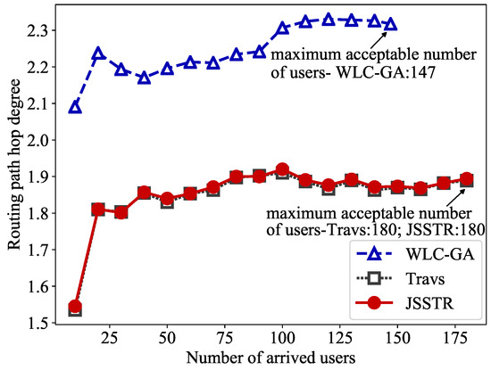
Figure 5. Routing path hop degree comparison for JSSTR, Travs and WLC-GA.

The above results were caused by the fact that the WLC-GA algorithm calculates the destination server without considering its impact on routing path calculation. More specifically, when using WLC-GA, the destination server is calculated by the WLC algorithm, and the weighted server status is the only factor considered in this process. After the destination server has been chosen, the GA algorithm can only calculate the routing path between that server and the user. This means that even it there is one more efficient routing path in the underlying network, if the server connected to that path is not chosen as the destination server, that path will not be taken as the final routing path. In contrast, when using the JSSTR algorithm, the destination server and routing path are calculated jointly. Thus, the destination server will be calculated based on the server status and network status. Therefore, the length of the routing path made by WLC-GA is bigger than that of JSSTR. Additionally, from that figure, it can be seen that the routing path hop degree of the JSSTR algorithm is almost the same as the Travs method, which indicates that the JSSTR algorithm can almost get the optimal result as the traversal-based method.

In addition, as the routing path degree made by JSSTR and Travs is less than WLC-GA, JSSTR and Travs can accept more users than WLC-GA. In the evaluation, when using JSSTR and Travs, the maximum acceptable number of users is 180. As mentioned above, all servers can serve at most 200 users in this evaluation; thus, it is the upper limit of users that the network can carry. Once the number of arrived users is larger than 180, even if the servers can serve more users, the subsequent arrived users will not be served as the network cannot transfer more traffic. For WLC-GA, the maximum acceptable number of users is 147, which decreases by about 22 percent compared to JSSTR and Travs.

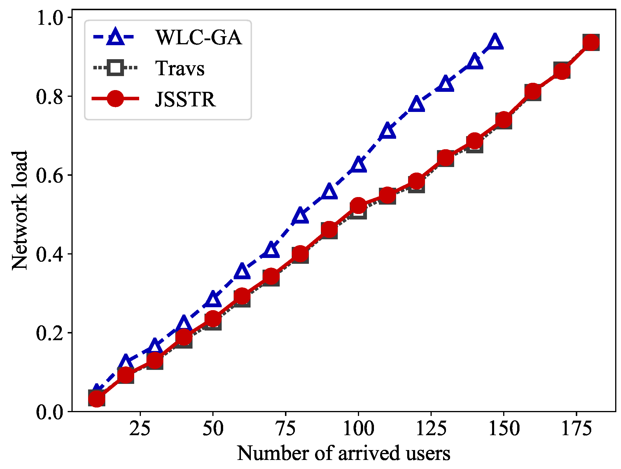
(2) Network load: The same analysis can be made for the curves given in Figure 6, which shows the network load values when using the JSSTR, WLC-GA and Travs algorithms. As shown in that figure, when the number of arrived users is the same, the network load values of JSSTR are obviously less than those of WLC-GA. For instance, when there are 100 users, the network load of JSSTR is 0.5226, while for WLC-GA, it is 0.6277. In that case, the network load decreases about 20 percent when using JSSTR. Thus, JSSTR can achieve higher efficiency than WLC-GA. Meanwhile, the network load values of JSSTR are almost the same as Travs, which shows that JSSTR can almost obtain the optimal result when calculating the routing path.

Figure 6. Network load comparison for JSSTR, Travs and WLC-GA.

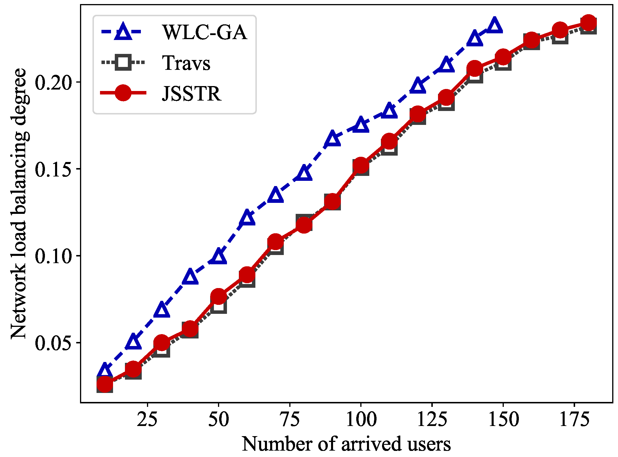
(3) Network load balancing degree: Figure 7 presents the network load balancing degrees of JSSTR, WLC-GA and Travs. From Figure 7, we can see that JSSTR outperforms WLC-GA and has as good performance as Travs. More precisely, for different numbers of users, the network load balancing degrees of JSSTR are always lower than those of WLC-GA. For instance, when the number of arrived users is 100, the network load balancing degree of JSSTR is 0.1521, while the network load balancing degree of WLC-GA is 0.1757. Therefore, in that case, compared with WLC-GA, JSSTR can decrease the network load balancing degree by about 16 percent. At the same time, the network load balancing degree of Travs is 0.1508, which is very close to the network load balancing degree of JSSTR. It shows that the JSSTR can almost obtain the optimal load balancing degree when calculating the routing path. As previously mentioned, when choosing the destination server, WLC-GA will choose one server from the server cluster without considering the network status. On the contrary, JSSTR will jointly calculate the destination server and routing path. Therefore, JSSTR can improve network efficiency and balance network load.

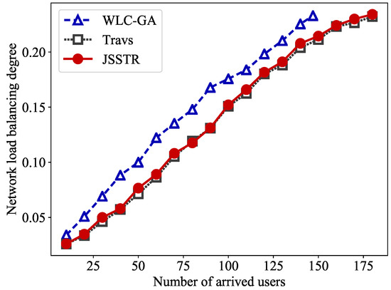
Figure 7. Network load balancing degree comparison for JSSTR, Travs and WLC-GA.

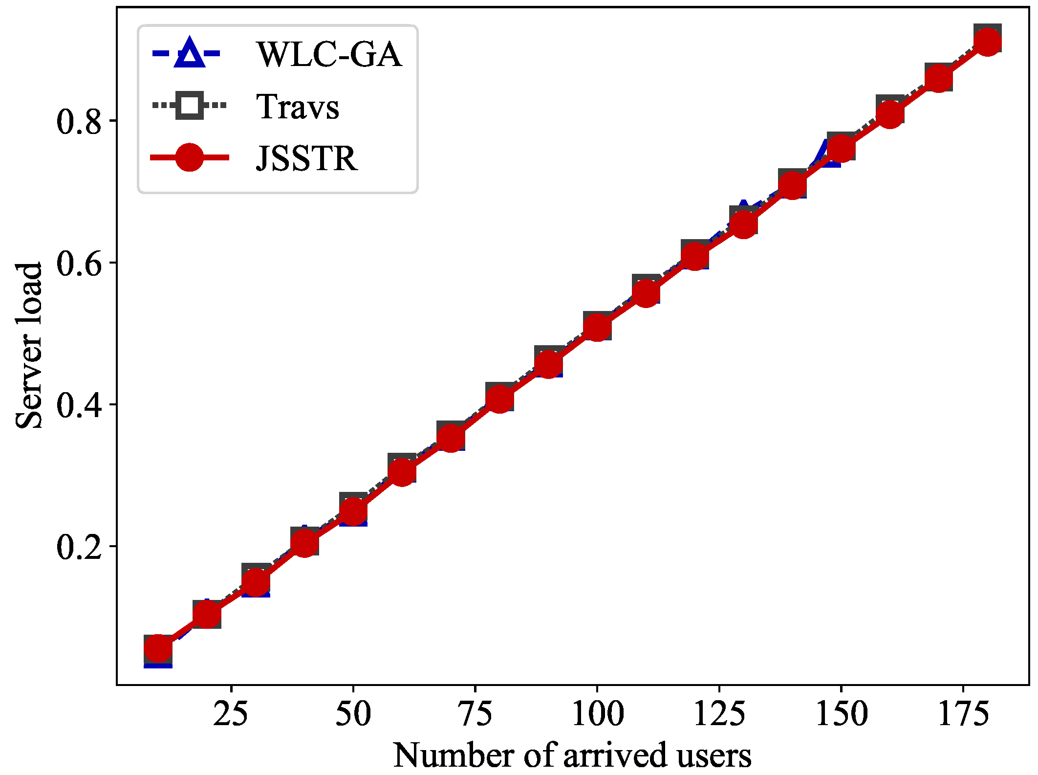
(4) Server load: From Figure 8, it can be seen that for JSSTR, WLC-GA and Travs, the server loads are nearly same. When the number of users is 100, the server loads of JSSTR, WLC-GA and Travs are 0.5083, 0.5114 and 0.5083, respectively. This indicates that compared with WLC-GA, the impact on server load generated by our JSSTR method is negligible. This is because our JSSTR method calculates the destination server and routing path jointly. Therefore, when choosing the destination server, the server fitness is considered as one of the main factors. If there are servers with a similar load, the server that has more path fitness will be chosen as the destination server, which will not impact the server load.

Figure 8. Server load comparison for JSSTR, Travs and WLC-GA.

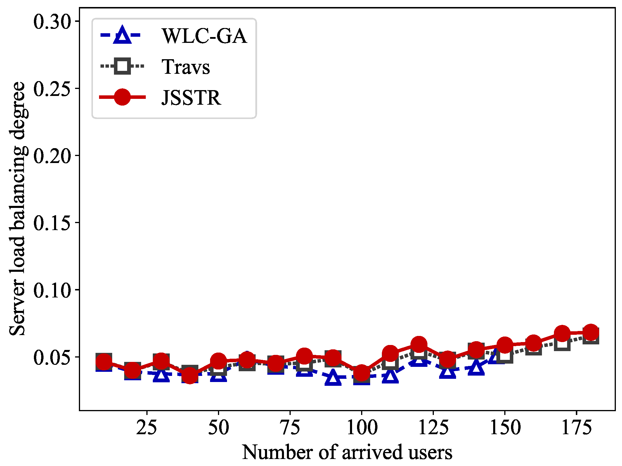
(5) Server load balancing degree: Figure 9 shows the server load balancing degrees of JSSTR, WLC-GA and Travs. The server load balancing degree of JSSTR is very close to that of WLC-GA and Travs. For example, when there are 100 users, the server load balancing degrees of JSSTR, WLC-GA and Travs are 0.0381, 0.0352 and 0.0369, respectively.

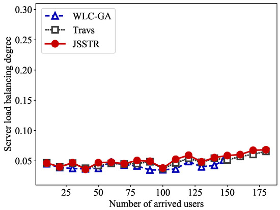
Figure 9. Server load balancing degree comparison for JSSTR, Travs and WLC-GA.

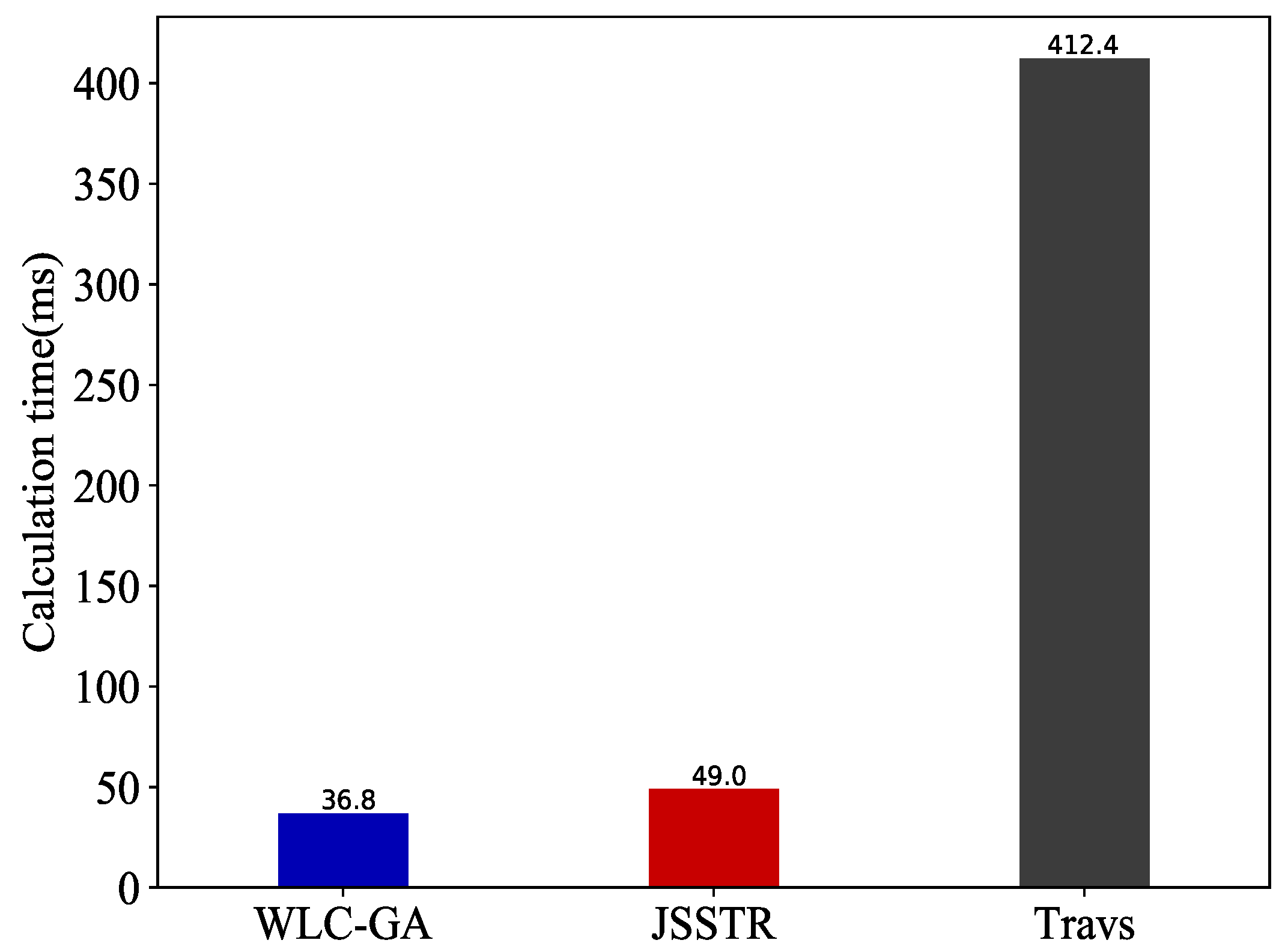
(6) Calculation time: Figure 10 is the result of the comparison of the computation complexity. In Figure 10, the calculation time is the mean time interval between the controller receiving the user request and successfully handling that user request. In Figure 10, we can see that the proposed JSSTR algorithm has a little increase in calculation time compared with WLC-GA (49.0 ms for JSSTR and 36.8 ms for WLC-GA). However, the mean calculation times of JSSTR is significantly less than that of the Travs algorithm (412.4 ms).

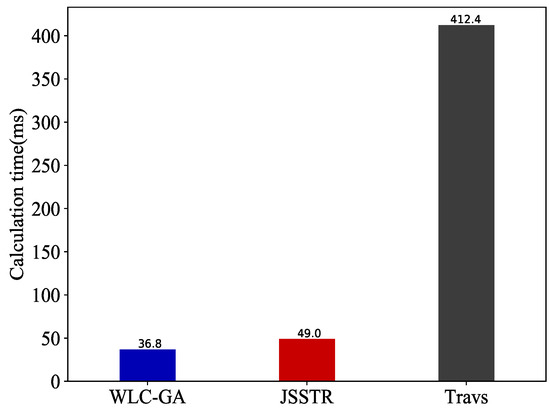
Figure 10. Calculation time comparison for JSSTR, Travs and WLC-GA.

Except these metrics, it should also be noted that in the proposed JSSTR algorithm, the number of memeplexes and number of frogs in each memeplex affect the calculation accuracy and computation complexity of that algorithm. The probability of finding the optimal (or sub-optimal) solution of the joint server selection and traffic routing problem increases as the number of memeplexes and number of frogs increase. However, the computational complexity of the JSSTR algorithm also increases with increasing the number of memeplexes and the number of frogs. Otherwise, as the number of memeplexes and frogs in each memeplex decreases, the calculation accuracy and computation complexity decrease.

Besides, compared with WLC-GA, the JSSTR and Travs algorithms need to collect server load information. However, the traffic generated by collecting server load information is rather small. For example, in a real scenario, when using the Simple Network Management Protocol (SNMP) to collect server load, the length of SNMP packets is usually less than 90 bytes. In order to collect the CPU utilization, RAM utilization and disk utilization, six SNMP packets will be generated. The server load information is usually collected every five seconds. Assume that there are 16 servers in the server cluster. In that case, the traffic speed generated by collecting servers’ load is about 13.5K bits per second, which is rather small compared to the bandwidth of the link.

In conclusion, all the above evaluation results and analysis indicate that JSSTR can achieve better network resource utilization and higher network load balancing with acceptable less increase in computation complexity compared with WLC-GA. Additionally, compared with the traversal-based method, it can achieve nearly the same network resource utilization, network load balancing, server resource utilization and server load balancing while clearly decreasing the computation complexity.

7. Conclusions

In order to avoid the inefficient use of network resources or some network issues caused by choosing the destination server from the server cluster without considering its impact on the network when handling user requests, the joint server selection and traffic routing problem has been proposed in this work. As that problem belongs to NP-hard problems, a heuristic algorithm called JSSTR has been proposed to find the approximate optimal solution of that joint server selection and traffic routing problem in polynomial time. The proposed JSSTR algorithm has been evaluated using Mininet. Several metrics including the routing path hop degree, network load, network load balancing degree, server load and server load balancing degree have been proposed and used to evaluate the proposed algorithm. The evaluation results showed that the proposed algorithm can achieve high network utilization, network load balancing and server load balancing simultaneously.

References

- Software-Defined Networking: The New Norm for Networks. Available online: https://www.opennetworking.org/ (accessed on 27 July 2018).
- Software-Defined Networking (SDN): Layers and Architecture Terminology. Available online: https://tools.ietf.org/html/rfc7426 (accessed on 27 August 2018).
- Jain, S.; Kumar, A.; Mandal, S.; Ong, J.; Poutievski, L.; Singh, A.; Venkata, S.; Wanderer, J.; Zhou, J.; Zhu, M.; et al. B4: Experience with a globally-deployed software defined WAN. ACM SIGCOMM Comput. Commun. Rev. 2013, 43, 3–14. [Google Scholar] [CrossRef]
- Wang, Y.W.; Chen, H.N.; Wu, X.L.; Shu, L. An energy-efficient SDN based sleep scheduling algorithm for WSNs. J. Netw. Comput. Appl. 2016, 59, 39–45. [Google Scholar] [CrossRef]
- Wang, Y.; Zhang, Y.; Chen, J. SDNPS: A load-balanced topic-based publish/subscribe system in software-defined networking. Appl. Sci. 2016, 6, 91. [Google Scholar] [CrossRef]
- Subedi, T.N.; Nguyen, K.K.; Cheriet, M. SDN-based fault-tolerant on-demand and in-advance bandwidth reservation in data center intercoonects. Int. J. Commun. Syst. 2018, 31, e3479. [Google Scholar] [CrossRef]
- Cui, Y.H.; Yan, L.S.; Xing, H.L.; Yang, H.; Chen, J.; Pan, W. SD-HDC: Software-Defined Hybrid Optical/Electrical Data Center Architecture. In Proceedings of the 2017 IEEE Global Communications Conference (GLOBECOM), Singapore, 4–8 January 2017. [Google Scholar]
- Yang, H.; Zhang, J.; Zhao, Y.L.; Ji, Y.F.; Li, H.; Lin, Y.; Li, G.; Han, J.R.; Lee, Y.; Ma, T. Performance evaluation of time-aware enhanced software defined networking (TeSDN) for elastic data center optical interconnection. Opt. Express 2014, 22, 17630–17643. [Google Scholar] [CrossRef] [PubMed]
- Cui, Y.H.; Yan, L.S.; Li, S.F.; Xing, H.L.; Pan, W.; Zhu, J.; Zheng, X.Y. SD-Anti-DDoS: Fast and efficient DDoS defense in software-defined networks. J. Netw. Comput. Appl. 2016, 68, 65–79. [Google Scholar] [CrossRef]
- Kaur, S.; Kumar, K.; Singh, J.; Ghumman, N.S. Round-robin based load balancing in Software Defined Networking. In Proceedings of the International Conference on Computing for Sustainable Global Development (INDIACom), New Delhi, India, 11–13 March 2015; pp. 2136–2139. [Google Scholar]
- Zhong, H.; Fang, Y.; Cui, J. Reprint of “LBBSRT: An efficient SDN load balancing scheme based on server response time”. Future Gener. Comput. Syst. 2018, 80, 183–190. [Google Scholar] [CrossRef]
- Eusuff, M.; Lansey, K.; Pasha, F. Shuffled frog-leaping algorithm: A memetic meta-heuristic for discrete optimization. Eng. Optim. 2006, 38, 129–154. [Google Scholar] [CrossRef]
- Chen, W.B.; Shang, Z.H.; Tian, X.N.; Li, H. Dynamic server cluster load balancing in virtualization environment with openflow. Int. J. Distrib. Sens. Netw. 2015, 11, 531–538. [Google Scholar] [CrossRef]
- Shang, Z.H.; Chen, W.B.; Ma, Q.; Wu, B. Design and implementation of server cluster dynamic load balancing based on OpenFlow. In Proceedings of the International Joint Conference on Awareness Science and Technology and Ubi-Media Computing (iCAST-UMEDIA), Aizuwakamatsu, Japan, 2–4 November 2013; pp. 691–697. [Google Scholar]
- OpenFlow Switch Specification 1.3.0. Available online: https://www.opennetworking.org/ (accessed on 27 July 2018).
- McKeown, N.; Anderson, T.; Balakrishnan, H.; Parulkar, G.; Peterson, L.; Rexford, J.; Shenker, S.; Turner, J. OpenFlow: Enabling innovation in campus networks. ACM SIGCOMM Comput. Commun. Rev. 2008, 35, 69–74. [Google Scholar] [CrossRef]
- Zhong, H.; Lin, Q.F.; Cui, J.; Shi, R.H.; Liu, L. An efficient sdn load balancing scheme based on variance analysis for massive mobile users. Mob. Inf. Syst. 2015. [Google Scholar] [CrossRef]
- Silva, W.J.A.; Dias, K.L.; Sadok, D.F.H. A performance evaluation of Software Defined Networking load balancers implementations. In Proceedings of the 31rd International Conference on Information Networking (ICOIN), Da Nang, Vietnam, 11–13 January 2017; pp. 132–137. [Google Scholar]
- The POX Controller. Available online: http://www.noxrepo.org (accessed on 27 July 2018).
- Zhang, H.; Guo, X. SDN-based load balancing strategy for server cluster. In Proceedings of the 3rd IEEE International Conference on Cloud Computing and Intelligence Systems (CCIS), Shenzhen/Hong Kong, China, 27–29 November 2014; pp. 662–667. [Google Scholar]
- Lantz, B.; Heller, B.; McKeown, N. A network in a laptop: Rapid prototyping for software-defined networks. In Proceedings of the 9th ACM SIGCOMM Workshop on Hot Topics in Networks (HotSDN), Monterey, CA, USA, 20–21 October 2010; p. 19. [Google Scholar]
- Mininet: An Instant Virtual Network on Your Laptop. Available online: http://mininet.org/ (accessed on 27 July 2018).
- Project Floodlight. Available online: http://www.projectfloodlight.org/ (accessed on 27 July 2018).
- Chen, S.L.; Chen, Y.Y.; Kuo, S.H. CLB: A novel load balancing architecture and algorithm for cloud services. Comput. Electr. Eng. 2017, 58, 154–160. [Google Scholar] [CrossRef]
- Sharifian, S.; Motamedi, S.A.; Akbari, M.K. A predictive and probabilistic load-balancing algorithm for cluster-based web servers. Appl. Soft Comput. 2011, 11, 970–981. [Google Scholar] [CrossRef]
- Baskett, F.; Chandy, K.M.; Muntz, R.R.; Palacios, F.G. Open, closed, and mixed networks of queues with different classes of customers. J. ACM 1975, 22, 248–260. [Google Scholar] [CrossRef]
- Lee, M.C.; Sheu, J.P. An efficient routing algorithm based on segment routing in software-defined networking. Comput. Netw. 2016, 103, 44–55. [Google Scholar] [CrossRef]
- Cheng, L.W.; Wang, S.Y. Application-aware SDN routing for big data networking. In Proceedings of the Global Communications Conference (GLOBECOM), San Diego, CA, USA, 6–10 December 2015; pp. 1–6. [Google Scholar]
- Yu, T.F.; Wang, K.; Hsu, Y.H. Adaptive routing for video streaming with QoS support over SDN networks. In Proceedings of the 29th International Conference on Information Networking (ICOIN), Siem Reap, Cambodia, 12–14 January 2015; pp. 318–323. [Google Scholar]
- Sendra, S.; Rego, A.; Lloret, J.; Jimenez, J.M.; Romero, O. Including artificial intelligence in a routing protocol using Software Defined Networks. In Proceedings of the IEEE International Conference on Communications, Paris, France, 21–25 May 2017; pp. 670–674. [Google Scholar]
- Tomovic, S.; Radusinovic, I. Fast and efficient bandwidth-delay constrained routing algorithm for SDN networks. In Proceedings of the NetSoft Conference and Workshops (NetSoft), Seoul, Korea, 6–10 June 2016; pp. 303–311. [Google Scholar]
- Tajiki, M.M.; Akbari, B.; Shojafar, M.; Mokari, N. Joint QoS and Congestion Control Based on Traffic Prediction in SDN. Appl. Sci. 2017, 7, 1265. [Google Scholar] [CrossRef]
- Celenlioglu, M.R.; Tuysuz, M.F.; Mantar, H.A. An SDN-based scalable routing and resource management model for service provider networks. Int. J. Commun. Syst. 2018, 31, e3530. [Google Scholar] [CrossRef]
- Yu, Y.S.; Ke, C.H. Genetic algorithm-based routing method for enhanced video delivery over software defined networks. Int. J. Commun. Syst. 2018, 31, e3391. [Google Scholar] [CrossRef]
- Liu, Y.; Pan, Y.; Yang, M.X.; Wang, W.Q.; Fang, C.; Jiang, R.J. The multi-path routing problem in the Software Defined Network. In Proceedings of the 11th International Conference on Natural Computation (ICNC), Garden Grove, CA, USA, 16–19 February 2015; pp. 250–254. [Google Scholar]
- Ferraz, L.H.G.; Mattos, D.M.F.; Duarte, O.C.M.B. A two-phase multipathing scheme based on genetic algorithm for data center networking. In Proceedings of the Global Communications Conference (GLOBECOM), Austin, TX, USA, 8–12 December 2014; pp. 2270–2275. [Google Scholar]
- Whitley, D. A genetic algorithm tutorial. Stat. Comput. 1994, 4, 65–85. [Google Scholar] [CrossRef]
- RYU SDN Framework. Available online: http://osrg.github.io/ryu/ (accessed on 27 July 2018).
- Singla, A.; Hong, C.Y.; Popa, L.; Godfrey, P.B. Jellyfish: Networking Data Centers, Randomly. In Proceedings of the USENIX Symposium on Networked Systems Design and Implementation (NSDI), San Jose, CA, USA, 3–5 April 2012; pp. 225–238. [Google Scholar]
- Shuai, L.; Xie, G.; Yang, J. Characterization of HTTP behavior on access networks in Web 2.0. Telecommunications. In Proceedings of the International Conference on ICT, Hong Kong, China, 7–8 July 2008; pp. 1–6. [Google Scholar]
- Waldmann, S.; Miller, K.; Wolisz, A. Traffic model for HTTP-based adaptive streaming. In Proceedings of the IEEE Conference on Computer Communications (INFOCOM), Atlanta, GA, USA, 1–4 May 2017; pp. 683–688. [Google Scholar]
© 2018 by the authors. Licensee MDPI, Basel, Switzerland. This article is an open access article distributed under the terms and conditions of the Creative Commons Attribution (CC BY) license (http://creativecommons.org/licenses/by/4.0/).