Abstract
One of the challenges in the field of remote sensing is how to automatically identify and classify high-resolution remote sensing images. A number of approaches have been proposed. Among them, the methods based on low-level visual features and middle-level visual features have limitations. Therefore, this paper adopts the method of deep learning to classify scenes of high-resolution remote sensing images to learn semantic information. Most of the existing methods of convolutional neural networks are based on the existing model using transfer learning, while there are relatively few articles about designing of new convolutional neural networks based on the existing high-resolution remote sensing image datasets. In this context, this paper proposes a multi-view scaling strategy, a new convolutional neural network based on residual blocks and fusing strategy of pooling layer maps, and uses optimization methods to make the convolutional neural network named RFPNet more robust. Experiments on two benchmark remote sensing image datasets have been conducted. On the UC Merced dataset, the test accuracy, precision, recall, and F1-score all exceed 93%. On the SIRI-WHU dataset, the test accuracy, precision, recall, and F1-score all exceed 91%. Compared with the existing methods, such as the most traditional methods and some deep learning methods for scene classification of high-resolution remote sensing images, the proposed method has higher accuracy and robustness.
1. Introduction
With the continuous development of remote sensing technology, a large number of high-resolution remote sensing images have been generated. How to effectively identify and classify high-resolution remote sensing images automatically has become a technical problem that needs to be solved urgently in the field of remote sensing [1]. High-resolution remote sensing image scene classification is widely used in land use, natural disaster monitoring, urban planning, computer mapping, vegetation mapping, geospatial target detection, and other applications [2,3,4].
In terms of abstraction level, scene classification of remote sensing images has experienced the development from pixel to object and then to the semantic scene [5]. In the early 1970s, the spatial resolution of satellite images was low, and the pixel size was usually larger and at most close to the size of the target of interest, so most remote sensing image analysis methods were based on per-pixel or even sub-pixel analysis [6]. With the development of remote sensing technology and the continuous improvement of spatial resolution, scene classification based solely on pixel-level encountered a bottleneck [7]. Therefore, researchers described and analyzed the object-level of remote sensing images. Although the performance of the object-level classification method is better than that of the pixel-level classification method, semantic information is not involved. Therefore, researchers began to analyze the semantic-level of scenes [7]. The scene image mentioned here refers to local image patches manually extracted from large-scale remote sensing images containing explicit semantic categories. Marking images according to semantic categories is the goal of semantic-level scene classification, and it is a challenging problem, because when describing a land cover image of a given category, there may be great variability in different scales and directions. With the refinement of classification, the problem of high intra-class variability and low inter-class distance becomes more and more serious [5].
For semantic-level remote sensing image scene classification, effective feature representation plays an important role in constructing a high-performance scene classification method. According to the features used in remote sensing scene classification, the existing remote sensing image scene classification methods can be divided into three categories: the methods based on low-level visual features, the methods based on middle-level visual features, and the methods based on high-level visual features [8]. Among them, low-level visual features mainly represent spectral, texture, shape, and spatial information of remote sensing images extracted by professionals. The usual methods are color histogram [9], texture descriptor, generalized search tree (GIST) [10], scale-invariant feature transformation (SIFT) [11], histogram of oriented gradient (HOG) [12], and so on. Low-level visual features are obtained by manual feature extraction. Due to the subjectivity of the selection of features and the semantic gap between semantic categories of the scene and low-level visual features, the scene classification methods based on low-level visual features are often not so effective when the remote sensing scene images become complex. Middle-level visual features include two cases. The first case is to abstract the low-level visual features by means of quantization and coding, such as bag of visual words (BoVW) [13], spatial pyramid matching (SPM) [14], probabilistic topic models (PTM) [15], Fisher vector coding [16], latent Dirichlet allocation (LDA) [17], etc. The second case is unsupervised feature learning, which can automatically learn features from a large number of unmarked data through a specific unsupervised learning algorithm, such as principal component analysis (PCA) [18], k-means clustering, sparse coding [19], autoencoder [20], etc. Middle-level visual features are the bridge between the lower-level visual features and semantic categories of scenes. The scene classification methods based on middle-level visual features have more advantages than the classification methods based on low-level visual features and still have great potential for the expression and abstraction of complex scene content features. High-level visual features refer to the use of the deep learning method to extract abstract semantic information of images. It is well known that deep learning, like the mechanism of the human brain, is a process of abstraction layer by layer. The low-level features of deep learning are features such as edges or colors, while higher level features are the abstraction of lower-level features, and the features extracted by top-level of the deep learning methods are the abstract semantic information of the previously mentioned features. At present, there are many deep learning models, such as deep belief network (DBN) [21], deep Boltzmann machine (DBM) [22], stacked autoencoder (SAE) [23], convolutional neural network (CNN) [24], and so on. The deep learning methods can fully mine the correlation between data, automatically learn the complex structure of high-dimensional data. Top-level features of deep learning also have the characteristic of semantic abstraction, which can establish direct mapping with semantic categories of scenes. All these characteristics make high-level visual features more suitable for semantic scene classification. The methods based on high-level visual features have achieved the best results in scene classification of high-resolution remote sensing images.
As the most important learning framework in scene classification, the convolutional neural network shows strong learning ability in scene classification of remote sensing images. Training new convolutional neural networks often requires a large amount of data. However, the number of images in the shared datasets of high-resolution remote sensing images is very limited, which fails to meet the requirements of designing an ideal model of convolutional neural network. In addition, it is difficult to train a new convolutional neural network, which requires high-performance computing devices and long training time. Therefore, there are relatively few related articles about training new convolutional neural networks with shared datasets of high-resolution remote sensing images. In order to further develop the deep learning methods in remote sensing image scene classification, it is necessary to construct new convolutional neural networks and conduct relevant researches.
In order to solve the problems existing in the field of scene classification of high-resolution remote sensing images, this paper proposes a scene classification method of high-resolution remote sensing images based on RFPNet. The main contributions of the paper are as follows:
- (1)
- The paper proposes a multi-view scaling strategy, which is a data amplification strategy, aiming to solve the problem of the limited number of images in the current high-resolution remote sensing image datasets. The difference between the multi-view scaling strategy and other dataset amplification methods is that different parts of the labeled boxes can be cropped randomly, and four interpolation algorithms are selected randomly to stretch the scale of the image, so as to serve as the input of the neural network. This method can not only enlarge the number of datasets, but also introduce noise through interpolation, thus improving the generalization ability of the convolutional neural network constructed.
- (2)
- This paper proposes the structure of RFPNet to learn high-level visual features of high-resolution remote sensing images for scene classification. The main characteristic of the RFPNet structure is to adopt the residual block, so that the accuracy will not reduce when adding more layers to the model constructed; The fusion strategy of pooling layer feature maps is proposed to ensure the integrity of information by solving the problem of information loss in the process of pooling. In order to further improve the accuracy of the model, the paper also uses the optimization methods of Dropout, parameter norm penalty, and the moving average model, to avoid the overfitting problem caused by the limited data in the existing high-resolution remote sensing image datasets.
The specific structure of this paper is as follows: there is a brief introduction on related work in Section 2; the proposed method is presented in Section 3; the experimental results of the proposed method on two benchmark datasets are presented in Section 4; the discussion is presented in Section 5; the conclusion is given in Section 6.
2. Related Work
In the following section, convolution neural networks and the application of convolution neural networks in remote sensing image scene classification are briefly introduced.
2.1. Convolutional Neural Network
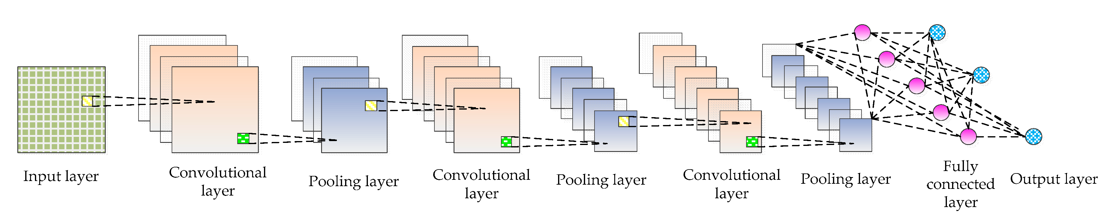
The convolutional neural network (CNN) was proposed by Fukushima [25] in 1980 and revised by LeCun [26]. In recent years, CNN has shown outstanding performance in natural language processing [27], disaster discovery [28], synthetic biomedicine [29], optical fiber communication [30], holographic image reconstruction [31], artificial intelligence program of go [32] and so on. With the advent of the era of big data, it is possible to train complex models with large-scale datasets on high-performance computing platforms (such as high-performance computers, graphics workstations, cloud computing platforms, etc.). In this context, many convolution neural network models have been proposed, such as LeNet [33], AlexNet [34], Overfeat model [35], VGGNet [36], GoogleNet [37], SPPNet [38], ResNet [39], MobileNets [40], ZFNet [41], DenseNet [42], and so on. CNN is a multi-layer network structure, whose basic structure mainly includes input layer, convolutional layer, pooling layer, fully connected layer, and output layer, as shown in Figure 1. The following are introduced in details.

Figure 1.
Basic structure of CNN.
- Input layer: The input layer is the input of the whole CNN. In the neural network of image processing, it generally represents the pixel matrix of the image.
- Convolutional layer: The convolutional layer is used to extract image features. Low-level convolutional layer extracts shallow features (such as edges, lines, and corners). High-level convolutional layer further learns abstract features through the input of low-level features. The convolutional layer obtains multiple feature activation maps by convolving the convolution kernel of a specific size with the previous layer, as shown in Equation (1).where represents the input image set, represents the jth feature map of the l layer, “*” represents the operation of convolution, is the ith feature map of the l-1 layer, represents the filter connecting the jth feature map of the l layer and the ith feature map of the l-1 layer, is the bias, represents the nonlinear activation function that can solve problems that cannot be solved by linear models. The activation functions commonly used include sigmoid, tanh, ReLU, etc. The calculation equation is as follows:
- Pooling layer: The introduction of a pooling layer is to reduce dimension and abstract the input image by imitating the human visual system. By sampling the convolved feature maps, the useful information of the image is preserved and the redundant data is removed, thus effectively preventing the overfitting problem and speeding up the computation speed. What’s more, the pooling layer has feature invariance which can make the model more concerned with the presence of certain features rather than the specific location of the features and tolerate some small displacement of features. There are generally two kinds of operations: maximum pooling and average pooling. The calculation equation of pooling layer is as follows:where is a sub-sampling function, represents the sub-sampling coefficient, represents the jth feature map in the l layer, is the ith feature map in the l-1 layer, is the bias, and represents the nonlinear activation function.
- Fully connected layer: The fully connected layer is usually used in the last layers of the network, which can combine the information transmitted in the former layers to achieve the explicit expression of classification.
- Output layer: CNN’s input image is passed over the layers of a convolutional layer, pooling layer, and fully connected layer, and it is finally passed through the classifier in the form of a category or probability. The logistic regression model is commonly used for binary classification problems, while the Softmax classifier is commonly used for multi-classification problems. The Softmax classifier is essentially a normalized exponential function. Assuming that the training set is composed of m tag samples , where . Supposing that the input data x is given, the probability value of j of each category needs to be estimated by using the hypothesis function whose equation is as follows:where is the parameter and the expression plays the role of normalization and ensures that the sum of probabilities of all categories is 1. The loss function of the whole system iswhere the function is defined as: , , . The gradient equation of the loss function is as follows:The parameter is updated by Equation (9), and the probability that x is classified as j is determined by Equation (10).
2.2. The Application of Convolution Neural Network in Remote Sensing Image Scene Classification
As an important learning framework in the field of computer vision, CNN has shown strong learning ability in remote sensing image scene classification. The classification research of remote sensing image scene based on deep convolutional neural networks appeared successively around 2015 [43,44]. The research methods in this field are mainly based on two ideas:
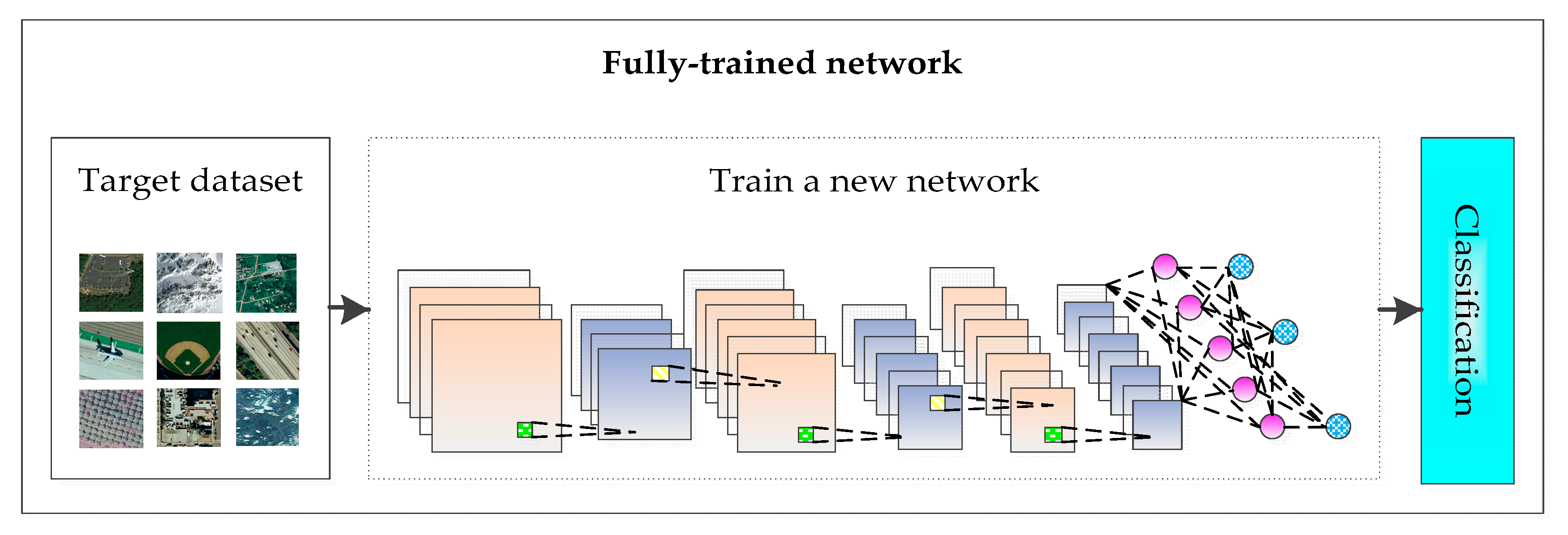
- Full-trained network: A new CNN is designed and trained based on the currently shared remote sensing image scene dataset, as shown in Figure 2.
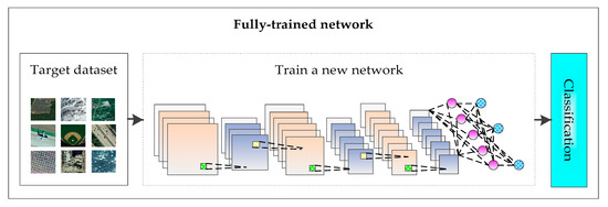 Figure 2. Full-trained network.
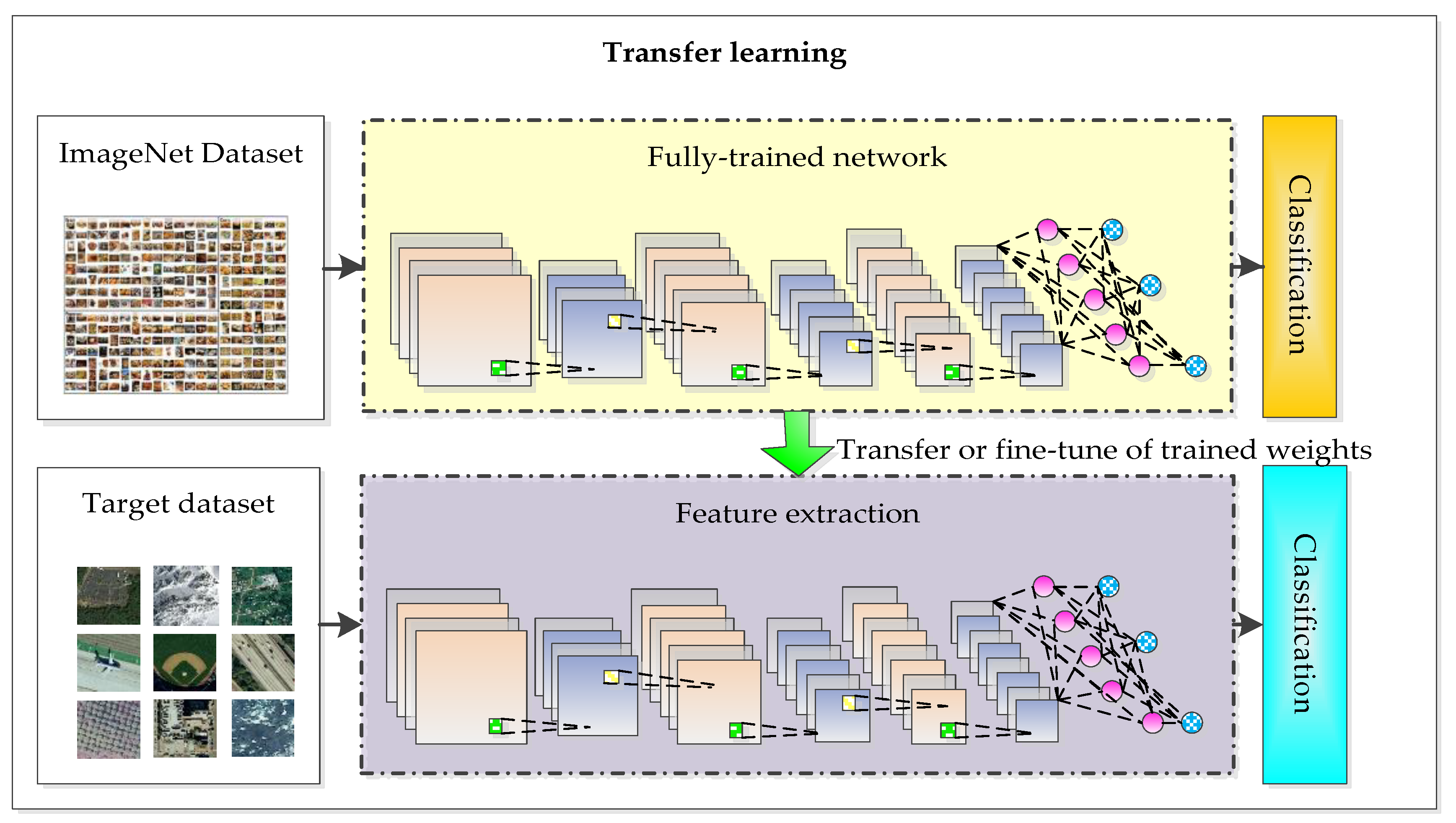
 - Transfer learning: The deep convolutional neural network model based on the large-scale image dataset is applied to remote sensing image scene classification directly or by fine-tuning, as shown in Figure 3.
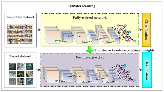 Figure 3. Transfer learning.
Based on the first idea, Luus et al. proposed a multiscale input strategy for multi-view deep learning and proved that the proposed method can improve prediction accuracy [43]. Basu et al. investigated the classification performance of convolutional neural networks with different depths on SAT-4 and SAT-6 datasets [45]. Zhang et al. proposed a gradient boosting random convolutional network (GBRCN) framework which can combine many deep neural networks effectively for scene classification and achieved good result [1]. Liu et al. proposed a deep random-scale stretched convolutional neural network (SRSCNN) for HSR remote sensing imagery and confirmed that the proposed method performs better than the traditional scene classification methods [46].
Based on the second idea, Castelluccio et al. fine-tuned CaffeNet and GoogleNet on the datasets of UC Merced and Brazilian Coffee Scenes to improve classification accuracy [5]. Hu et al. used AlexNet, CaffeNet, VGGNet, and PlacesNet to extract the features of high-resolution remote sensing images, the results revealed that the features from pre-trained CNNs generalize well and are more expressive than the low-level and mid-level features [44]. Zhang et al. used pre-trained CNN models including AlexNet, VGGNet, and GoogleNet to extract features of remote sensing datasets, and used linear support vector machine (SVM) to classify the remote sensing scene categories [8]. Marmanis et al. adopted OverFeat network to extract features and sent features into the CNN classifier for supervised learning, so as to solve the limited-data problem [47]. Nogueira et al. performed experiments with six popular convolutional neural networks using three remote sensing datasets and obtained good results [48]. Liu et al. fine-tuned VGG deep networks to classify high-resolution remote sensing images, which significantly reduced training times and computing burden as well [49].
The method of transfer learning, which is commonly used in most articles, will generally produce higher classification results compared with the full-trained network method. Since the method of building a new CNN model is driven by the target task, it can theoretically generate more accurate features and complete the classification task better. However, the number of high-resolution remote sensing images in the shared datasets is limited, so the classification accuracy is relatively low. At present, there are only a few works on the structural design of CNN based on shared remote sensing image datasets. However, in order to further develop the method of deep learning in high-resolution remote sensing scene classification, it is necessary to construct a new convolutional neural network based on the existing datasets.
3. Proposed Method
In this paper, a scene classification strategy using the full-trained network method based on shared high-resolution remote sensing datasets is proposed. This section is divided into three parts: (1) Multi-View Scaling Strategy; (2) The Structure of RFPNet; (3) Optimization Methods.
3.1. Multi-View Scaling Strategy
Training new convolutional neural networks often requires a large amount of data. However, the amount of data in the existing high-resolution remote sensing datasets is still limited, which cannot meet the requirements of designing an ideal CNN model. Therefore, this paper proposes a dataset amplification method—multi-view scaling strategy. Since high-resolution remote sensing images are a snapshot of the earth, objects on the surface of the earth are usually randomly distributed in the scene. As a result, the distribution mode of surface objects with different perspectives and scales is also very important for the scene classification of high-resolution remote sensing images.
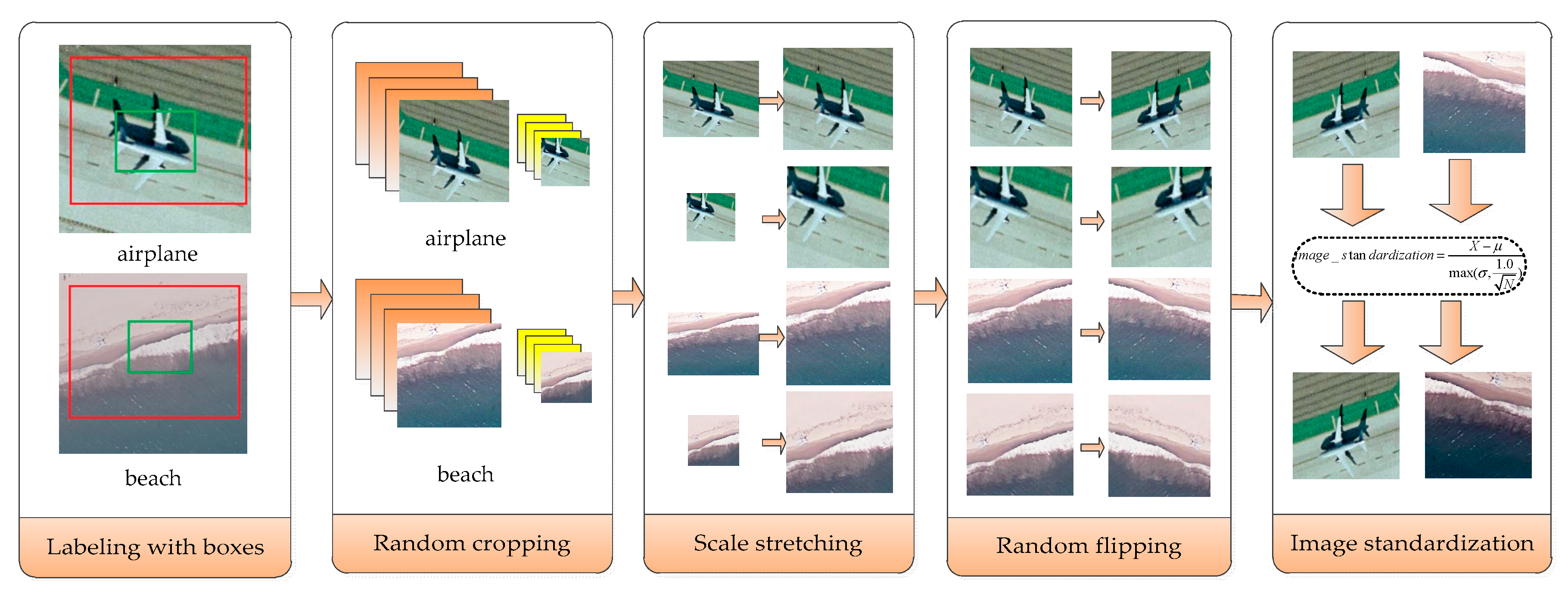
In fact, in order to solve the problem of limited labeled data in the field of high-resolution remote sensing image scene classification, many dataset amplification methods have been proposed. Different from the method of cutting the four corners and the center of the images to increase the number of labeled data proposed in [43], the basic idea of the multi-view scaling strategy proposed in this paper is to randomly cut the training data of high-resolution remote sensing image into different sizes and then stretch them. The specific steps are shown in Figure 4.
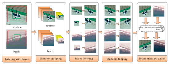
Figure 4.
Schematic diagram of the multi-view scaling strategy.
- Labeling with boxes: In order to extract different information from different perspectives, high-resolution remote sensing images are labeled with two boxes.
- Random cropping: Different parts of the labeled boxes are cropped randomly and get different pictures each time.
- Scale stretching: Four different size adjustment algorithms, including bilinear interpolation, nearest neighbor interpolation, bicubic interpolation, and area interpolation method, are used to stretch the intercepted image, so that the stretched image is the size of the input layer of the constructed convolutional neural network.
- Random flipping: Flip the image randomly with a certain probability.
- Image standardization: Normalize the image, so that the mean brightness value becomes 0 and the variance becomes 1, as shown in Equation (11).where represents the image matrix, represents the mean value of the image, represents the standard variance and represents the number of pixels in the image.
3.2. The Structure of RFPNet
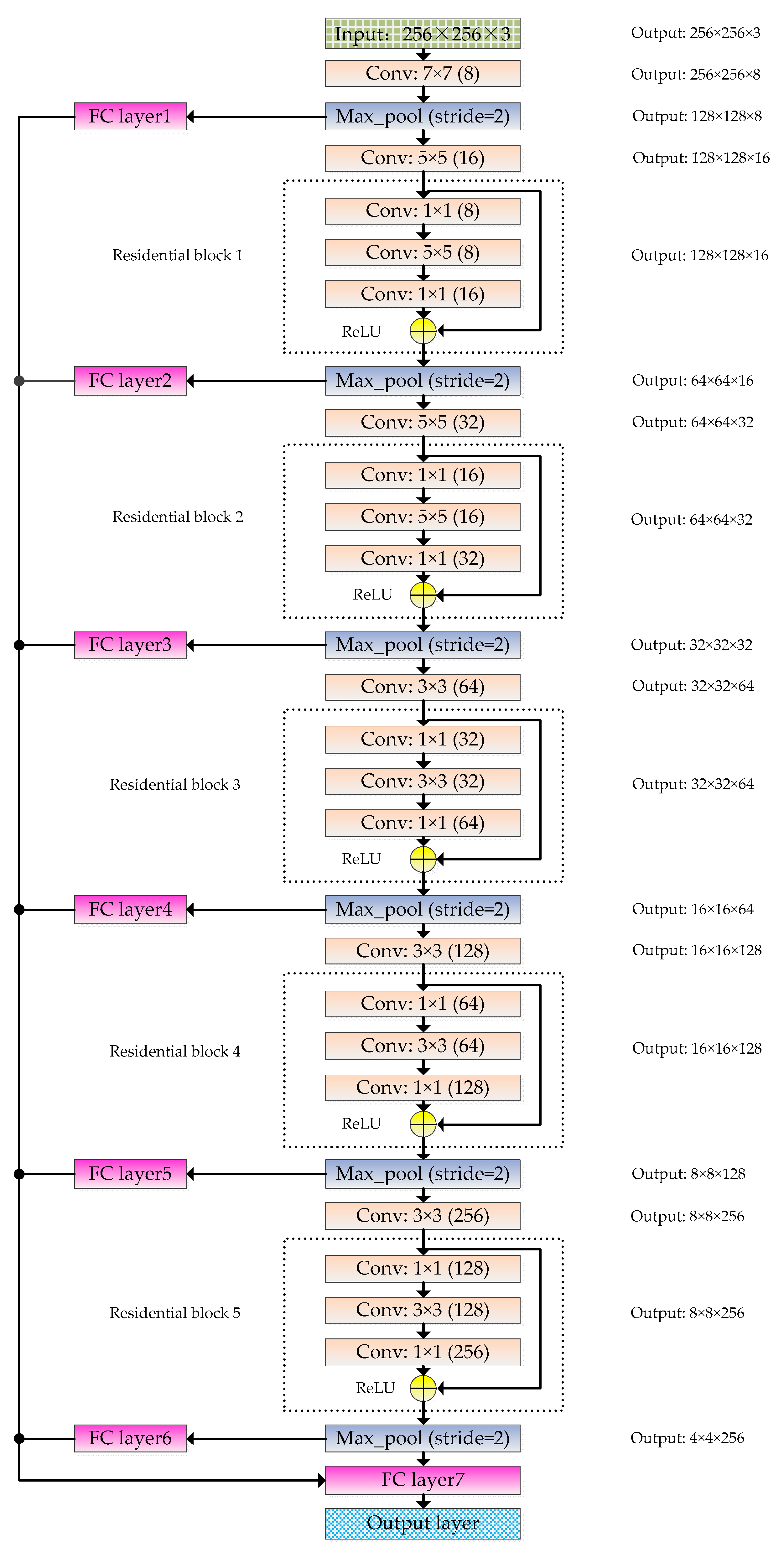
The RFPNet is based on the residual block and fusion strategy of pooling layer feature maps. The overall structure is shown in Figure 5. The RFPNet consists of an input layer, 21 convolutional layers, 6 pooling layers, 7 fully connected layers, and 1 output layer. The basic principle of RFPNet construction is that the lower layers of the model use large convolutional kernels to extract shallow features, and the higher layers of the model use small convolutional kernels to extract deep features. The input of RFPNet is 256 × 256 × 3 pixels. Next, a 7 × 7 convolutional kernel is used to extract large features. A maximum pooling layer is used to reduce dimension. A 5 × 5 convolutional kernel is then used to extract features that are relatively smaller than the features extracted by the 7 × 7 convolutional kernel. After that, a residual block (each residual block contains three convolutional layers) is used. Next, a maximum pooling layer is used to reduce feature dimensions. Through a number of convolutional layers, residual blocks, and pooling layers, the features are feed into the fully connected layer named FC layer7. In order to solve the problem of information loss caused by the pooling operation, each maximum pooling layer is transformed into a one-dimensional feature vector by using a fully connected layer, and then the vectors are cascaded and served as the input of a fully connected layer named FC layer7, thus ensuring the integrity of information to a certain extent. Finally, a Softmax classifier is used in the output layer of the model to complete the classification task. The output size depends on the number of remote sensing scene classification categories. Subsequently, the residual block and fusion strategy of pooling layer feature maps are introduced in detail respectively.
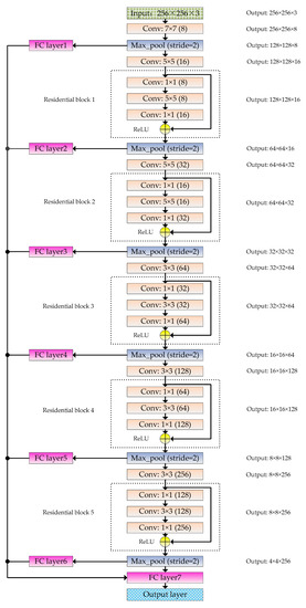
Figure 5.
Schematic diagram of the RFPNet structure. Where, Conv is the abbreviation of convolutional layer, Max_pool is the abbreviation of max-pooling layer, and FC layer is the abbreviation of fully connected layer.
3.2.1. The Residual Block
With the development of deep learning technology, CNN has made a breakthrough in the field of image classification. However, as the depth of the convolutional neural network model increases, gradient disappearance or gradient explosion will occur and even cause degradation if the depth is continuously deepened. In this context, ResNet was proposed in 2015 and has been used widely. Existing network modules of ResNet series include Resnet-18, Resnet-34, Resnet-50, Resnet-101, Resnet-152, and so on.
ResNet consists of several residual blocks which can greatly improve network performance. The main characteristic of the residual block is to introduce shortcut connections, which are those parts skipping one or more layers, thus making the learning goal of the network become the minimization of residuals. Assuming that the input of the multi-layer network is x and the expected mapping output is H(x), the optimization objective changes from fitting output H(x) to fitting the difference between output and input H(x)-x. The plain network and the residual block are shown in Figure 6. The plain network is to learn a complete output, while the residual block is to learn the difference between the output and input.
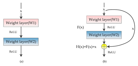
Figure 6.
The contrastive image of the plain network and the residual block: (a) the plain network; (b) the residual block.
In the residual block, what the residual mapping learned can be expressed as follows:
where represents the nonlinear function ReLU, and the biases are omitted for the sake of convenience. The output expression of the residual block is determined by Equation (13).
Although shortcut connections are used, Equation (13) does not introduce new parameters and increase the calculation amount. It should be noted that the and in Equation (13) must have the same dimension. When the input and output dimensions need to be changed, such as changing the number of channels, the linear transformation of x can be made in the shortcut connection and then connected to the following layer, the expression is as follows:
The partial derivative Equation (13) is as follows:
It can be seen from Equation (15) that the residual block is highly sensitive to small changes.
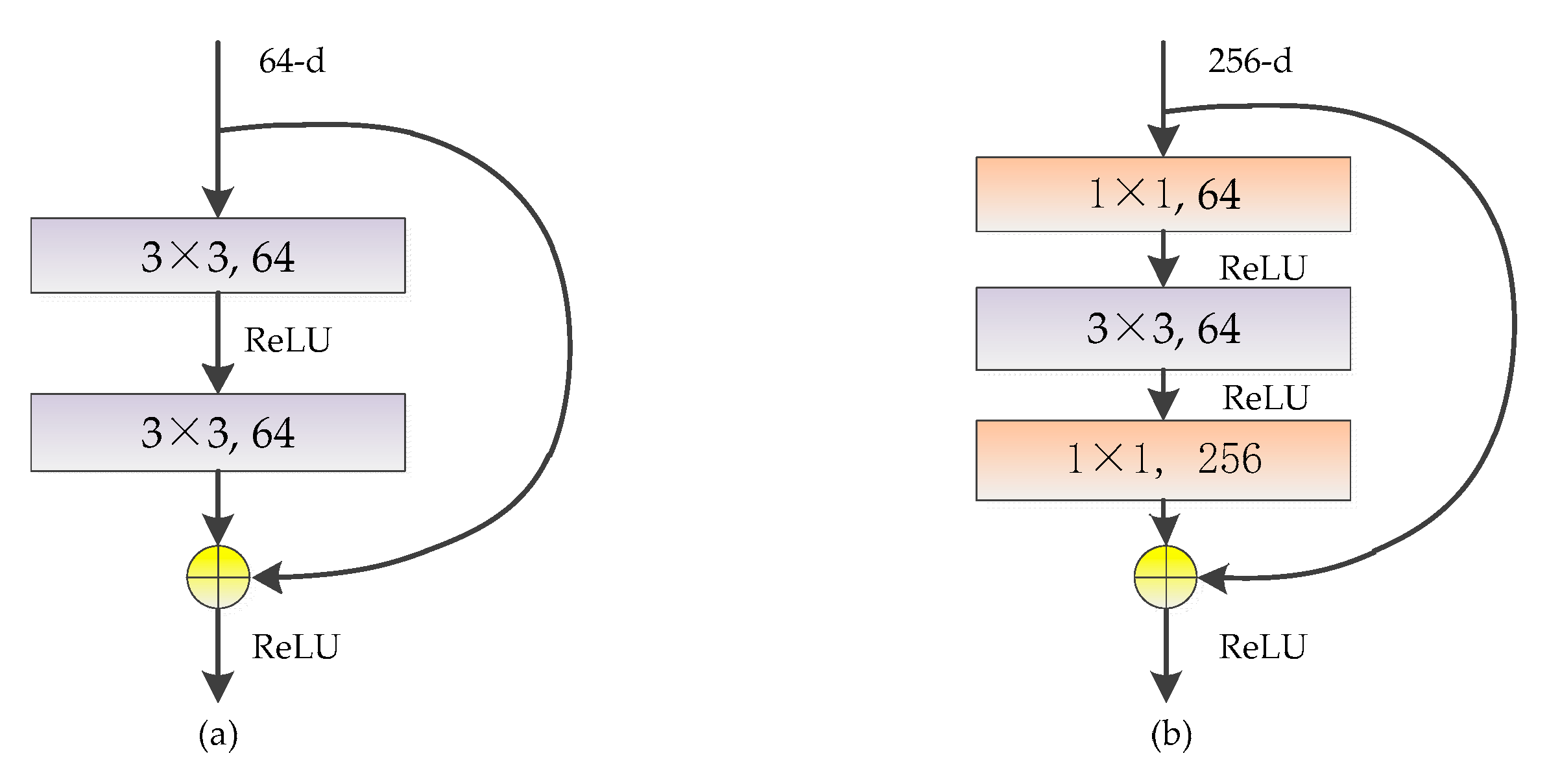
There are two kinds of typical structures of the residual block named 2-layer residual block and 3-layer residual block, as shown in Figure 7. In the 2-layer residual block, the input of the kth layer is connected with the output of k+2th layer by shortcut connection, and their vector addition result is taken as the input of k+3th layer. Since only vectors with the same dimension can be added, the dimensions of feature maps are reduced and increased in the 3-layer residual block by two 1 × 1 convolutional kernels.
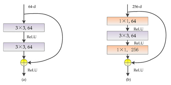
Figure 7.
Two kinds of typical structures of the residual block: (a) 2-layer residual block; (b) 3-layer residual block.
3.2.2. Fusion Strategy of Pooling Layer Feature Maps
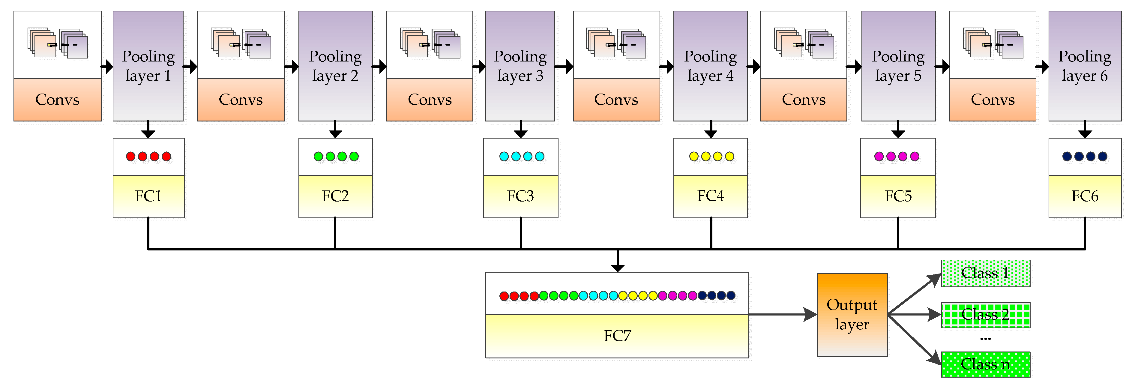
Although the pooling layer has the effect of characteristic invariance and dimension reduction, dimension reduction will lead to the loss of useful information and the detail information will be ignored. Based on this problem, this paper proposes the fusion strategy of pooling layer feature maps, as shown in Figure 8. The features in each pooling layer are expanded into a one-dimensional vector through a fully connected layer. Features are then cascaded through the final fully connected layer. Finally, classification is carried out through the output layer. This strategy can make the semantic information contained in different pooling layers complement each other and retain the details, thus improving the classification accuracy.

Figure 8.
Schematic diagram of the fusion strategy of pooling layer feature maps.
3.3. Optimization Methods
In the training process of CNN, when there are too many parameters in the model but the training data is limited, it is easy to produce the phenomenon that the gap between training error and the test error is too large, that is, the overfitting problem. Therefore, Dropout strategy and parameter norm penalty are adopted to avoid overfitting, and the moving average model is adopted to make the model more robust.
3.3.1. Dropout
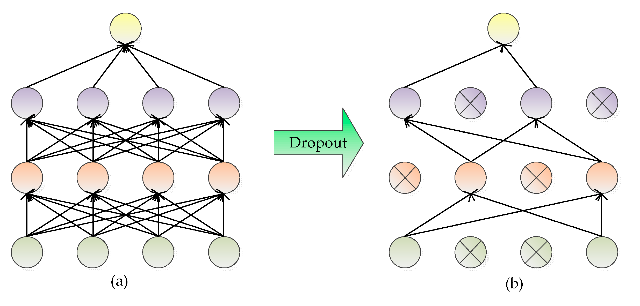
The basic principle of Dropout is to lose part of hidden layer neurons each time, which is equivalent to training on different networks each time, thus effectively reducing the interdependence between neurons, as shown in Figure 9. By adding the Dropout strategy, the calculation method of forwarding propagation changes from Equation (1) into Equation (17).
where Equation (16) indicates that each value in the vector is a Bernoulli distribution with probability generating values of 0 and 1, that is, each layer of the model blocks part of the input vector of l-1th layer through the vector , making the model approximate to the sub-network model sampled by the overall network model and the output of lth layer is obtained by forward propagation. The weight updating in the backpropagation stage is also carried out on the subnetwork model obtained by sampling.
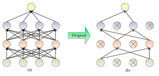
Figure 9.
Schematic diagram of Dropout: (a) a standard neural network; (b) the neural network using Dropout.
The Dropout strategy is added after fully connected layer named FC layer7 in the RFPNet to weaken the mutual adaptability and overfitting problem of network neurons, thus improving the generalization ability of the model.
3.3.2. Parameter Norm Penalty
The basic idea of parameter norm penalty is to add a parameter norm penalty that describes the complexity of the model into the loss function , the regularized loss function is shown in Equation (18).
where is the parameter that measures the proportion of norm penalty term in the regularized loss function. By using the strategy of parameter norm penalty, the model cannot arbitrarily fit the random noise in the training data. The effects are different with different parameter norm whose regularization methods include L1 regularization and L2 regularization. Where L1 regularization represents the sum of the absolute values of all the elements in the vector, as shown in Equation (19). While L2 regularization is the sum of squares of each parameter, as shown in Equation (20). In this paper, L2 regularization is adopted.
3.3.3. Moving Average Model
The moving average model controls the amplitude of the variable update by constantly updating the decay rate, which makes the model update faster at the initial stage of training and slower when it is close to the optimal value. The decay rate and parameter update are shown in Equations (21) and (22).
where init_decay is the initial decay rate, num_update is the number of model updates, shadow_var is the value of the variable after the update, and var is the variable to be updated.
4. Results
In this part, the experimental setup is introduced firstly. A variety of evaluation indicators are then used to comprehensively evaluate the experimental results. In order to prove the effectiveness of the proposed method, experiments were conducted on UC Merced and SIRI-WHU datasets. Furthermore, the accuracy of the proposed method is compared with traditional methods and deep learning methods. In order to verify the method proposed in this paper, seven models are created for relevant verification. For the sake of simplicity, each model is named according to its characteristic, as shown in Table 1. The following is a detailed explanation.

Table 1.
The models created for verification.
(a) WMS-RFPNet represents the convolutional neural network with RFPNet structure and all optimization methods but without the multi-view scaling strategy.
(b) MFPNet represents the convolutional neural network that adopts the multi-view scaling strategy, fusion strategy of pooling layer feature maps, and all optimization methods, but does not use the residual block.
(c) MRNet represents the convolutional neural network that adopts the multi-view scaling strategy, the residual block, and all optimization methods but does not adopt the fusion strategy of pooling layer feature maps.
(d) WD-RFPNet represents the convolutional neural network with the multi-view scaling strategy, RFPNet structure, parameter norm penalty, and the moving average model, but without the Dropout strategy.
(e) WPNP-RFPNet represents the convolutional neural network with the multi-view scaling strategy, RFPNet structure, Dropout, and the moving average model, but without the parameter norm penalty strategy.
(f) WWAM-RFPNet represents the convolutional neural network with the multi-view scaling strategy, RFPNet structure, Dropout, and parameter norm penalty, but without the moving average model.
(g) RFPNet represents the proposed method with the multi-view scaling strategy, RFPNet structure, and all optimization methods.
4.1. Experiment Settings
This paper conducted experiments on the UC Merced dataset and the SIRI-WHU dataset, which are adopted for the following three reasons:
(1) As benchmark datasets, these two datasets are widely used in the field of high-resolution remote sensing image classification, so as to facilitate the comparison with the methods proposed by other scholars.
(2) These two datasets contain a relatively small number of images, so it can further prove the advantages of the dataset amplification method proposed in this paper.
(3) The two datasets are acquired by different sensors and contain scene images of different regions. Therefore, experiments using these two different datasets can further prove the generalization ability of the proposed method.
In the experiment, 80% of high-resolution remote sensing images were randomly selected as the training set, and the remaining 20% was used as the test set. The batch size which refers to the number of samples selected for a training iteration was set to 64. The regulation rate of L2 regulation was set to 0.0001. The initial decay rate of the moving average model was set to 0.9999. The training iteration is set to 100,000. The experimental hardware platform was based on Intel E5-2680 V3 processor, TITAN V GPU, 64G memory. The software platform of the experiment was based on Ubantu16.04, and adopted CUDA 9.0, CUDNN 7, and TensorFlow1.12.0 environment.
4.2. Evaluation Indicators
Accuracy is a common indicator for classification evaluation, but the proposed method cannot be comprehensively evaluated based on accuracy alone. Therefore, the paper uses accuracy, precision, recall, and F1-score as the evaluation indicators. For a sample classification problem with a number of M, which contains P positive examples, and N negative examples, the sample can be divided into four cases according to the combination of real category and the predicted category: true positive (TP), false positive (FP), true negative (TN), and false negative (FN).
Among them, TP is the positive example predicted to be positive, and the FN is the positive example predicted to be negative, so the number of the positive example P is
Similarly, TN is the negative example judged to be negative, and FP is the negative cases predicted to be positive, so the number of the negative example N is
The accuracy is the proportion of correct cases, and the calculation equation is
Precision is the proportion of truly positive examples in all cases predicted to be positive examples. The calculation equation is
Recall is the proportion of all positive examples predicted to be positive examples, and the calculation equation is
F1-score is the comprehensive evaluation indicator of precision and recall, and the calculation equation is
4.3. The Analysis of Test Results on the UC Merced Dataset
The UC Merced dataset [50] collected by the United States Geological Survey (USGS) is used to prove the effectiveness of the proposed method. It contains 21 kinds of land scene with 100 images in each category and covers various urban areas around the United States, as shown in Figure 10. The size of each image is 256 × 256 pixels and the spatial resolution is about 30 cm. The UC Merced dataset presents highly overlapping categories, such as “dense residential area”, “sparse residential area”, and “medium residential area”, which further increases the difficulty of classification.
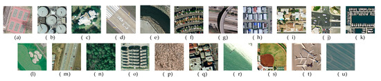
Figure 10.
Sample of 21 class UC Merced dataset: (a) tennis court; (b) storage tanks; (c) sparse residential; (d) runway; (e) river; (f) parking lot; (g) overpass; (h) mobile home park; (i) medium residential; (j) intersection; (k) harbor; (l) golf course; (m) freeway; (n) forest; (o) dense residential; (p) chaparral; (q) buildings; (r) beach; (s) baseball diamond; (t) airplane; (u) agricultural.
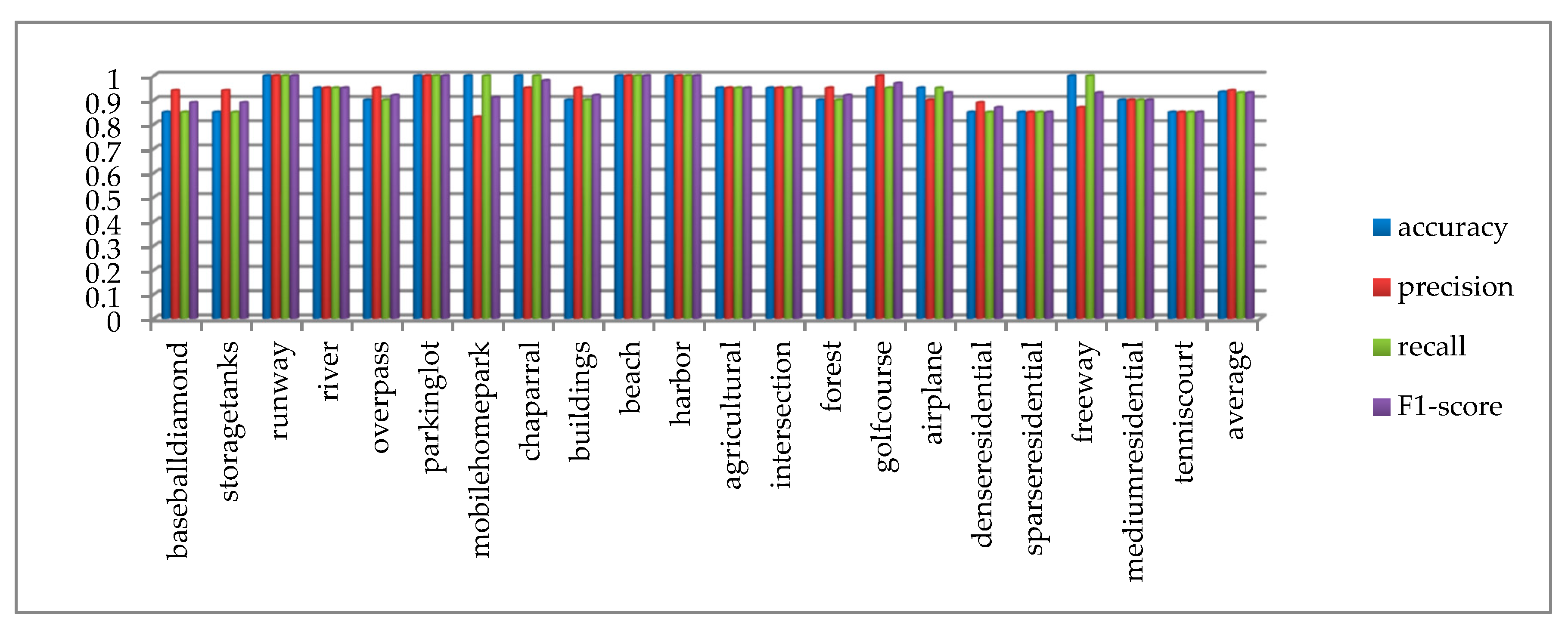
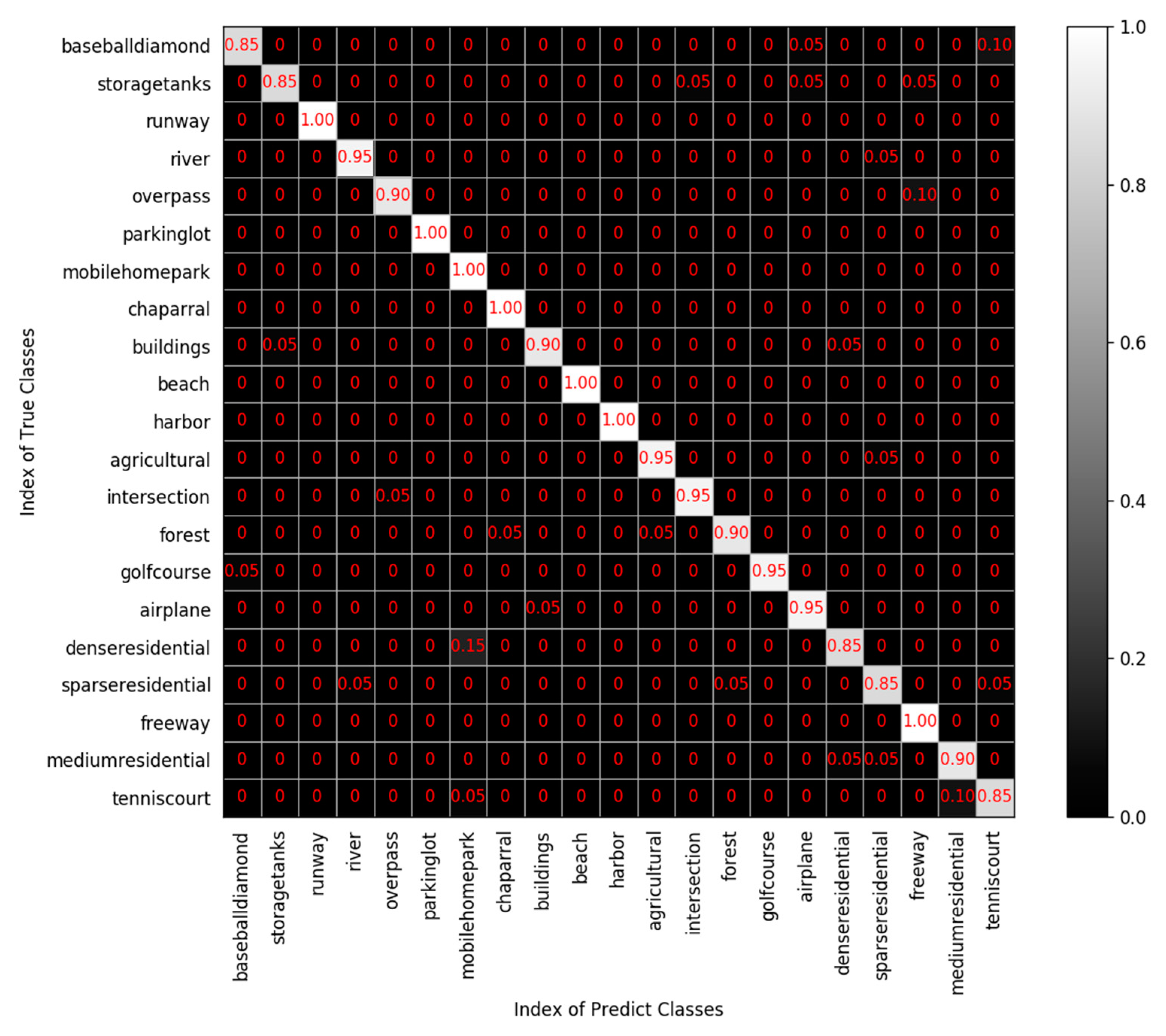
Multiple indicators are used to evaluate the result, as shown in Figure 11. The accuracy, precision, recall, and F1-score of each category all exceed 80%. The average accuracy, average precision, average recall, and average F1-score of all categories are 93.3%, 94%, 93%, and 93%, respectively, which proves that the proposed method has comprehensive advantages. The confusion matrix of the UC Merced dataset is shown in Figure 12, from which we can see that the classification accuracy of a single category ranged from 85% to 100%. The categories with 100% classification accuracy are runway, parking lot, mobile home park, chaparral, beach, harbor, and freeway, which further proves the high performance of the proposed method.
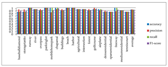
Figure 11.
Test result of accuracy, precision, recall, F1-score on the UC Merced dataset.
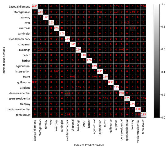
Figure 12.
Confusion matrix of the UC Merced dataset.
In order to prove the effectiveness of the proposed method, the accuracy of the proposed method is compared with traditional methods and deep learning methods on the UC Merced dataset. Different evaluation indexes were used in the articles for comparison, but accuracy was used as their general evaluation index. Therefore, in order to compare with other methods, the paper only compares the accuracy so as to illustrate the advantages of the proposed method. As shown in Table 2, the method proposed in the paper has achieved good results. Traditional methods mentioned in this paper refer to the scene classification methods of high-resolution remote sensing images based on the low-level visual features and the middle-level visual features. SPCK [51], BOVW [50], BRSK [52], SPMK [14], Bag-of-SIFT [53], SPM [54], SAL_LDA [55], UFL [56], MinTree+KD-Tree [57] and Partlets [58] all belong to the scene classification methods of high-resolution remote sensing images based on middle-level visual features, and their accuracy is almost lower than that of the deep learning methods, let alone the methods based on low-level visual features. Low-level visual features have certain limitations in the semantic information description of scene classification. Compared with the classification methods based on low-level features and high-level features, although the implementation process of the classification methods based on low-level visual features is relatively simple, the classification accuracy is the lowest. The presentation of middle-level visual features bridged the gap between low-level features and semantic categories of scenes. Compared with the classification methods based on low-level features, the classification methods based on middle-level features can improve the classification accuracy, but the implementation process will be more complex. Compared with the classification methods based on high-level features, the methods based on middle-level visual features still have some problems in the expression of semantic categories. The methods of high-level visual features can avoid artificial feature selection and automatically learn potential features from data. Therefore, the classification accuracy of the deep learning methods is generally higher than that of the traditional methods. However, the methods based on deep learning require a lot of data for training, which takes a long time and has high requirements for computer storage. Among deep learning methods such as LPCNN [59], CNN with Overfeat feature [47], WMS-RFPNet, MRNet, MFPNet, WD-RFPNet, WPNP-RFPNet, WMAM-RFPNet, and RFPNet, RFPNet has the highest classification accuracy for the following reasons:
Table 2.
Comparison of classification methods based on the UC Merced dataset.
(1) The multi-view scaling strategy was adopted, and, thus, the CNN model can learn the characteristics of the remote sensing images of different perspectives. On one hand the multi-view scaling strategy is a method of dataset amplification, on the other hand the stretching method in the multi-view scaling strategy is equivalent to adding noise in the process of the inputting data, which can improve the generalization ability of the model. As shown in Table 2, the classification accuracy of RFPNet is 31.66% higher than that of WMS-RFPNet, which proves that the effectiveness of the multi-view scaling strategy for high-resolution remote sensing image scene classification.
(2) The adoption of the residual block greatly simplified the learning objective and the training difficulty, and made it possible to deepen the network layer without reducing the accuracy rate. As shown in Table 2, the classification accuracy of RFPNet is 4.52% higher than that of MFPNet, which proves the effectiveness of the adoption of the residual block in scene classification of high-resolution remote sensing images.
(3) The fusion strategy of pooling layer feature maps was adopted to cascade the features, which ensured the integrity of information and solved the problem of information loss caused by the pooling operation of traditional CNN. As can be seen in Table 2, the classification accuracy of RFPNet is 5.95% higher than that of MRNet, thus, proving the effectiveness of fusion strategy of pooling layer feature maps.
(4) Dropout was adopted to randomly delete some hidden units, thus improving the generalization ability of the model and reducing the phenomenon of overfitting. As can be seen in Table 2, the classification accuracy of RFPNet is 5.95% higher than that of WD-RFPNet, thus proving the effectiveness of using Dropout strategy.
(5) The parameter norm penalty strategy was adopted to control the complexity of the model by adding penalty terms to the objective function, so as to solve the problem of overfitting. As can be seen in Table 2, the classification accuracy of RFPNet is 2.38% higher than that of WPNP-RFPNet, thus proving the effectiveness of using parameter norm penalty strategy.
(6) The moving average model was adopted to make the final model more robust. As can be seen in Table 2, the classification accuracy of RFPNet is 4.28% higher than that of WMAM-RFPNet, thus proving the effectiveness of using the moving average model.
Compared with other deep learning methods like LPCNN [59], CNN with Overfeat feature [47], and so on, the proposed method also has its advantages.
4.4. The Analysis of Test Result on the SIRI-WHU Dataset
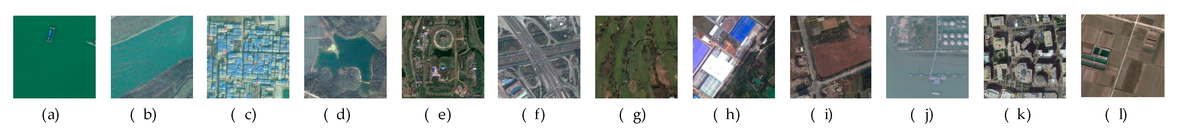
In order to prove the effectiveness of the proposed method, the experiment was also carried out on the SIRI-WHU dataset. The SIRI-WHU dataset [60] is Google’s 12 class image dataset. It was collected by the remote sensing group of Wuhan university from Google Earth and mainly covers urban areas in China. The size of each image is 200 × 200 pixels and the spatial resolution is 2 m. Each category of the dataset has 200 images, as shown in Figure 13. Since satellite images in Google Earth are not a single data source, but the integration of satellite images and aerial data, the images are different from those in the UC Merced dataset.
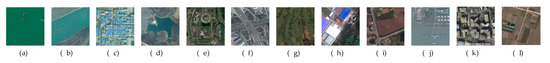
Figure 13.
Sample of 12 class Google image dataset of SIRI-WHU: (a) water; (b) river; (c) residential; (d) pond; (e) park; (f) overpass; (g) meadow; (h) industrial; (i) idle land; (j) harbor; (k) commercial; (l) agriculture.
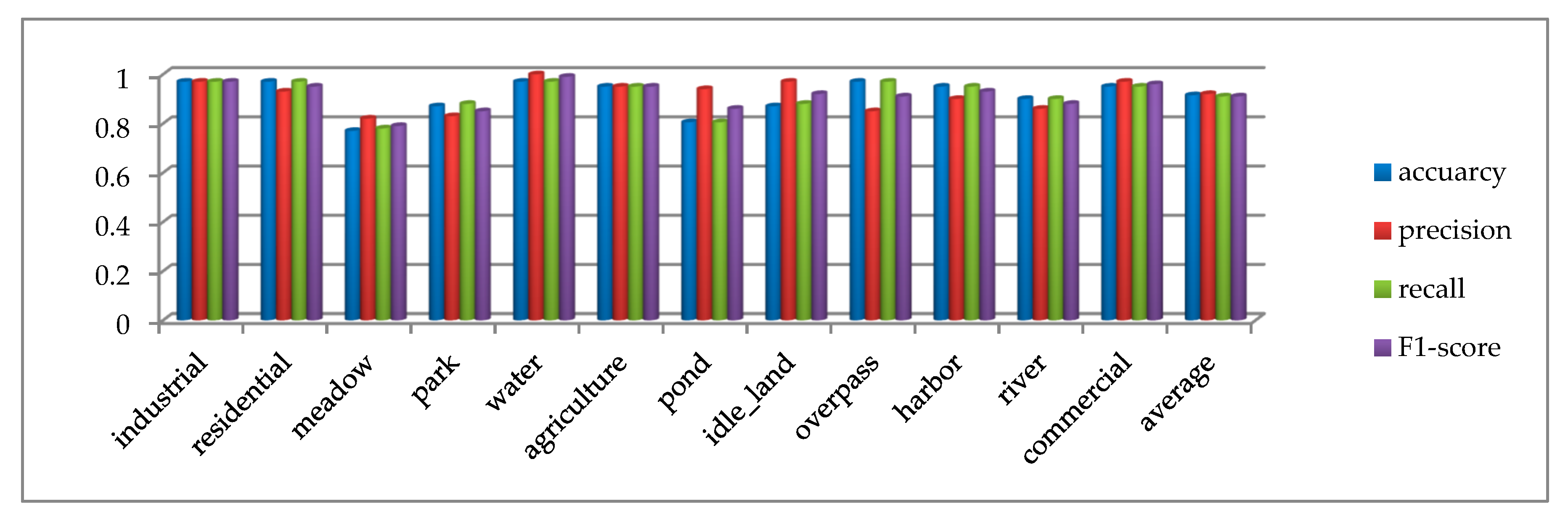
Multiple indicators are used to evaluate the result on the SIRI-WHU dataset, as shown in Figure 14. In addition to meadow, the accuracy, precision, recall, and F1-score of other categories all exceed 80%. The average accuracy, average precision, average recall and average F1-score of all categories are 91.5%, 92%, 91%, and 91%, respectively, which further proves that the proposed method has comprehensive advantages. The confusion matrix of the SIRI-WHU dataset is shown in Figure 15a, from which we can see that the classification accuracy of a single category ranged from 77% to 97%. The categories with 97% classification accuracy are industrial, residential, water, and overpass, which further proves the high effectiveness of the proposed method. The reason for the accuracy of SIRI-WHU dataset is lower than that of UCM dataset is analyzed as follows: as can be seen in Figure 15a, the classification accuracy of pond was only 80% and 10% pictures are misclassified as rivers. Worse still, the meadow classification accuracy is the lowest among other categories and 12% pictures were misclassified into parks. As can be seen in Figure 15b, the similarity between ponds and rivers leads to low classification accuracy. As for meadow and park, the park is basically composed of meadow, there is little difference between the two categories. In a word, the SIRI-WHU dataset is challenging due to the high similarity between classes, and the good results on the SIRI-WHU dataset indicate the feasibility of the proposed method.
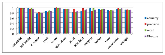
Figure 14.
Test result of accuracy, precision, recall, F1-score on the SIRI-WHU dataset.
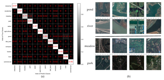
Figure 15.
(a) Confusion matrix of the SIRI-WHU dataset. (b) Image categories that can be easily misclassified.
In order to prove the effectiveness of the proposed method, the accuracy of the proposed method is compared with traditional methods and deep learning methods on the SIRI-WHU dataset. As accuracy is the general evaluation index of other comparison methods, this paper only compares the accuracy of different methods. As shown in Table 3, the method proposed in the paper on the SIRI-WHU dataset has achieved good results. Traditional methods mentioned in this paper also refer to the scene classification methods of high-resolution remote sensing images based on low-level visual features and middle-level visual features. SPM [14], LDA [17], PLSA [61], S-UFL [62], SIFT+BoVW [63], and RF [64] are all high-resolution remote sensing scene classification methods based on middle-level visual features, and their accuracy is mostly lower than that of deep learning methods, let alone the methods of low-level visual features. The method of features integration [65] fuses low-level visual features with middle-level visual features to improve the accuracy of scene classification, but the accuracy is still lower than the method proposed in this paper. Because there is a semantic gap between low-level visual features and scene semantic categories, the scene classification methods based on low-level visual features often fail to achieve good results. Although middle-level visual features are abstract expressions of low-level visual features, there are still some gaps between middle-level visual features and semantic categories of scenes. High-level visual features extracted by deep learning methods can simulate the human brain mechanism to interpret data and obtain better features. Therefore, the classification accuracy of the deep learning method is generally higher than that of the traditional methods. Among deep learning methods such as LPCNN [59], WMS-RFPNet, MRNet, MFPNet, WD-RFPNet, WPNP-RFPNet, WMAM-RFPNet, and RFPNet, RFPNet has the highest classification accuracy. Further analysis can be made through Table 3:
Table 3.
Comparison of classification methods based on the SIRI-WHU dataset.
(1) The classification accuracy of RFPNet is 8.3% higher than that of WMS-RFPNet, which proves that the effectiveness of the multi-view scaling strategy for high-resolution remote sensing image scene classification.
(2) The classification accuracy of RFPNet is 4.98% higher than that of MFPNet, which proves the effectiveness of the adoption of the residual block in scene classification of high-resolution remote sensing images.
(3) The classification accuracy of RFPNet is 2.83% higher than that of MRNet, thus proving the effectiveness of the fusion strategy of pooling layer feature maps.
(4) The classification accuracy of RFPNet is 3.5% higher than that of WD-RFPNet, thus proving the effectiveness of using the Dropout strategy.
(5) The classification accuracy of RFPNet is 0.87% higher than that of WPNP-RFPNet, thus proving the effectiveness of using the parameter norm penalty strategy.
(6) The classification accuracy of RFPNet is 1.07% higher than that of WMAM-RFPNet, thus proving the effectiveness of using the moving average model.
Even compared with other methods of deep learning like LPCNN [59] and so on, the proposed method still has very good results.
5. Discussion
Due to the importance of accuracy in the field of scene classification, this paper only introduced the influence of each parameter on accuracy in this section. Learning rate, Dropout rate, the feature length of the fully connected layer and the training iterations are all important parameters of CNN and play an important role in classification accuracy. In Section 5.1, the influence of four different learning rates on classification results is discussed. In Section 5.2, experiments were conducted for seven different Dropout rates to analyze the best accuracy. In Section 5.3, the feature length of the fully connected layer is evaluated. In Section 5.4, the test results corresponding to different iteration steps in the training process are analyzed.
5.1. Analysis in Relation to Learning Rate
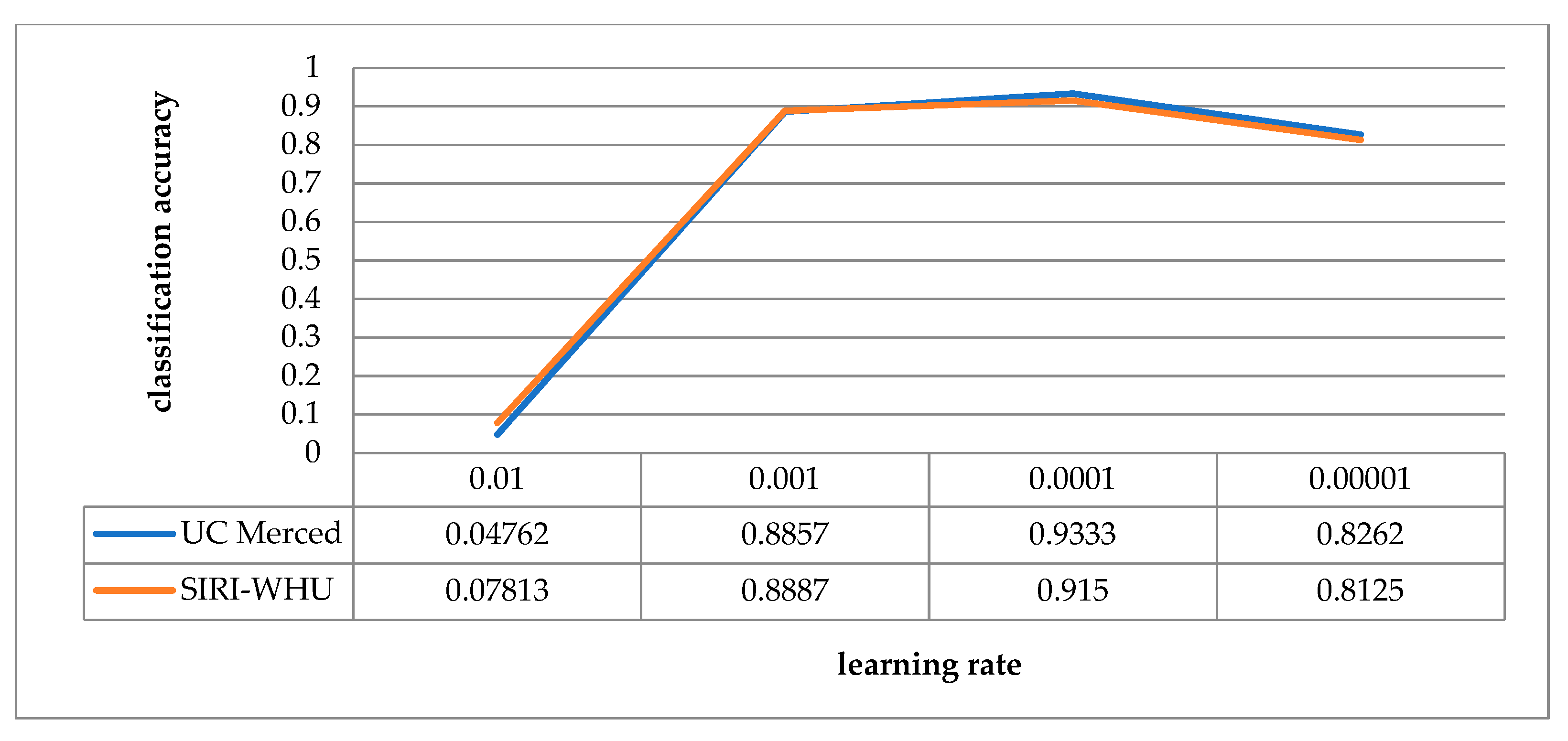
In this paper, the Adam optimization algorithm is adopted to carry out gradient descent, which required the setting of learning rate. Learning rate determines how far the weights will move in the gradient direction in a batch. If the learning rate is very low, the optimization time will become very long. On the contrary, if the learning rate is high, the training may not converge. In order to test the influence of different learning rates on the classification accuracy of RFPNet, experiments were carried out on the UC Merced dataset and the SIRI-WHU dataset respectively. With other parameters of RFPNet network unchanged, the learning rate is adjusted to 0.01, 0.001, 0.0001, and 0.00001, as shown in Figure 16. The trend of the UC Merced dataset’s accuracy is roughly the same as that of the SIRI-WHU dataset. When the learning rate is set to 0.01, the classification results of the two datasets diverge. When the learning rate is 0.0001, the training accuracy reaches the best result, and when the learning rate is 0.00001, it is in a declining trend.
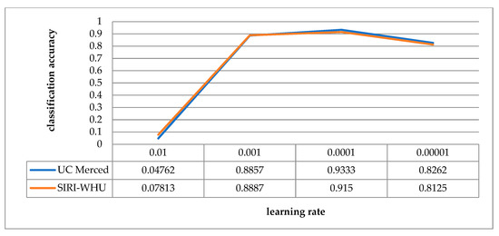
Figure 16.
Schematic diagram of the classification accuracy corresponding to different learning rates.
5.2. Analysis in Relation to Dropout Rate
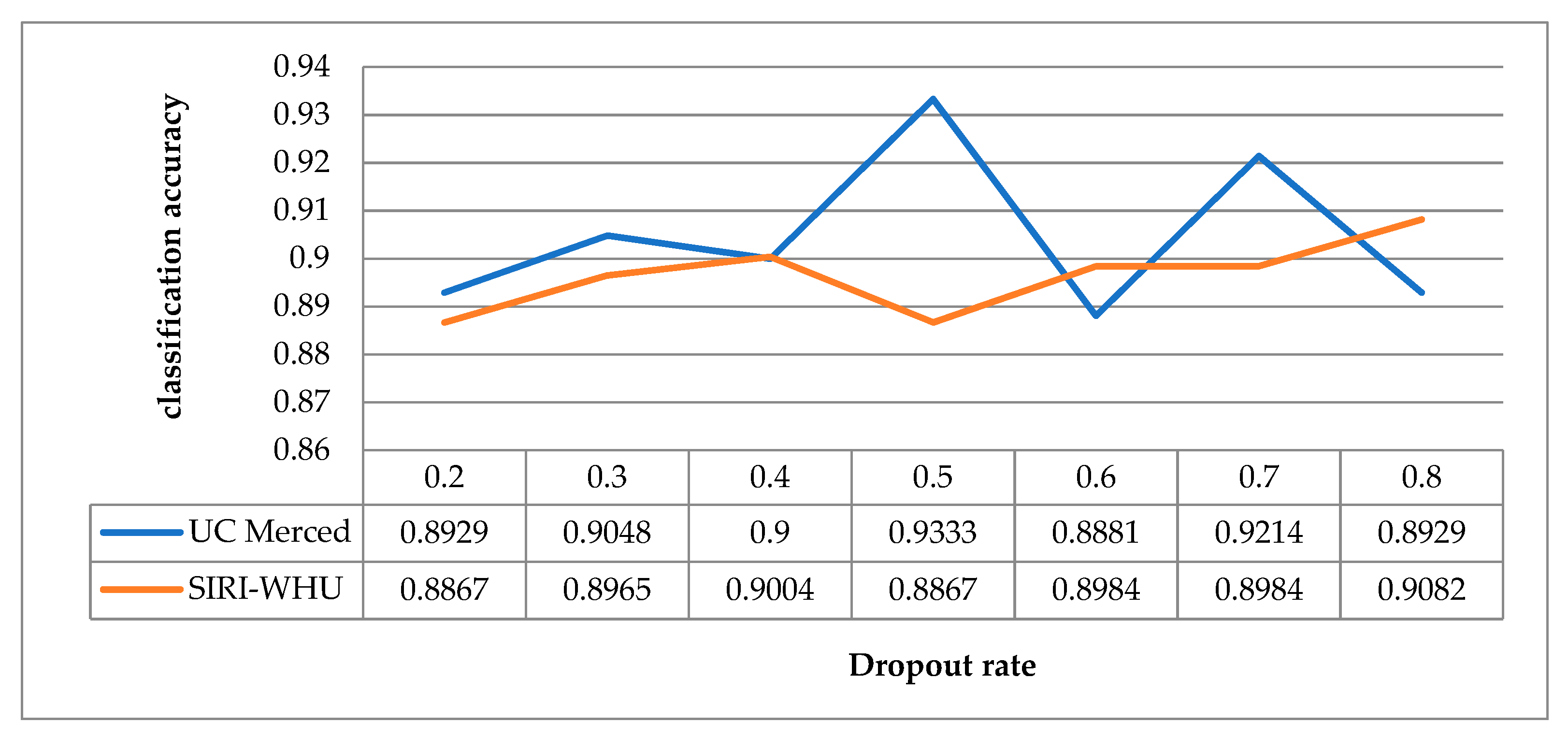
In the Dropout strategy, the Dropout rate p is the probability for one neuron to be discarded, and the probability to be retained is 1-p. The larger p is, the more features will be discarded during feature selection. The Dropout rates ranging from 0.2 to 0.8 were trained on the UC Merced dataset and the SIRI-WHU dataset respectively under the condition of keeping other parameters unchanged. The experimental results are shown in Figure 17. It can be seen that the classification accuracy of UC Merced dataset is the highest when the Dropout rate is 0.5. For the SIRI-WHU dataset, the classification accuracy is optimal when the Dropout rate is 0.8. It indicates that the optimal Dropout rate may not be the same when using the same model and different datasets.
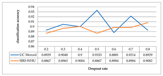
Figure 17.
Schematic diagram of the classification accuracy corresponding to different Dropout rates.
5.3. Analysis in Relation to the Feature Length of the Fully Connected Layer
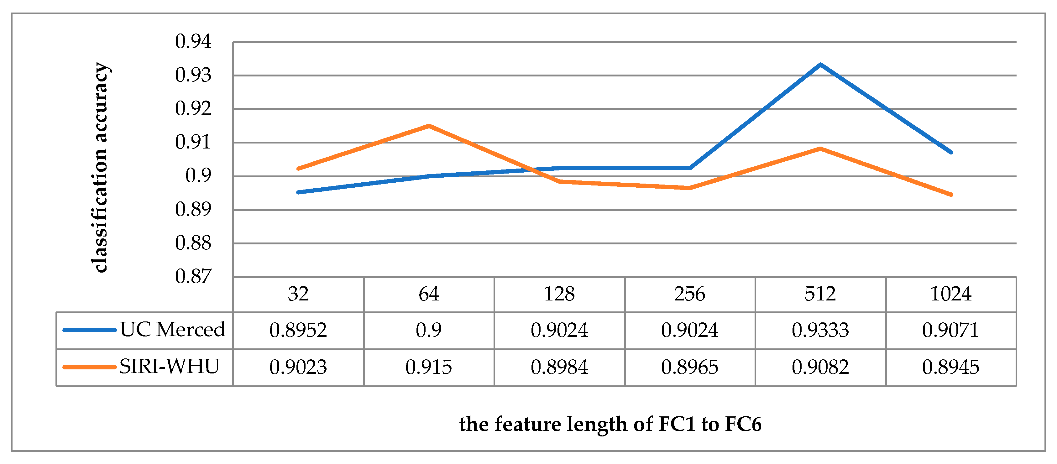
The main function of the fully connected layer is to map the learned representation of features into the sample tag space. Increasing the feature length of the fully connected layer is equivalent to increasing the number of neurons, which can theoretically improve the learning ability of the model. However, if the feature length of the fully connected layer is too long, which, on one hand, will make the learning ability too strong and lead to overfitting, on the other hand, will increase the operation time and reduce the efficiency. In order to test the influence of feature length on classification accuracy, the feature length of the fully connected layers from FC1 to FC6 is set as exponential multiples of 32, 64, 128, 256, 512, 1024 with other parameters unchanged, as shown in Figure 18. When the feature length from FC1 to FC6 is 512, the classification accuracy is the highest on UCM dataset. For the SIRI-WHU dataset, when the feature length from FC1 to FC6 is 64, the convolutional neural network has the best feature expression ability.
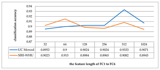
Figure 18.
Schematic diagram of the classification accuracy corresponding to the feature length of the fully connected layer.
5.4. Analysis in Relation to the Training Iterations
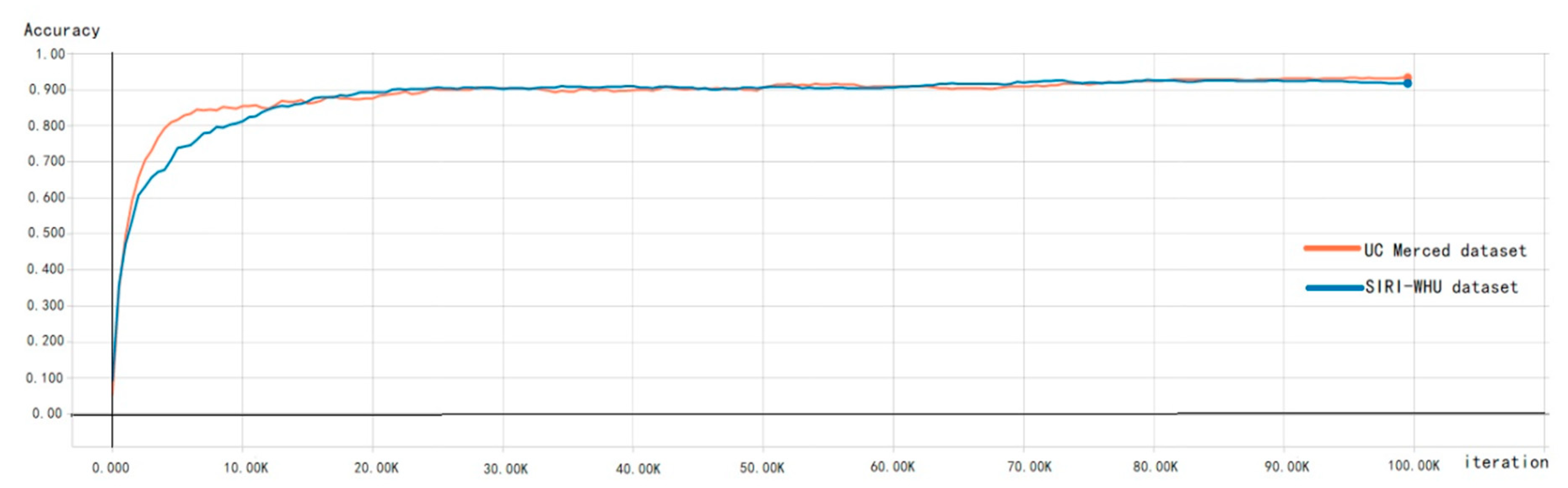
The concept of iteration is the process of training once with a batch of samples. In order to analyze the influence of different training iterations on test results, the corresponding experiments were carried out. As shown in Figure 19, the accuracy of both the UC Merced dataset and SIRI dataset has not changed significantly after about 25,000 iterations, and the accuracy then increases slowly, steadily, and slightly. In the paper, with the adoption of the residual block, there is no gradient explosion or gradient disappearance in the testing process, which indicates the advantages of the proposed method again.
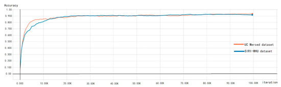
Figure 19.
Schematic diagram of the classification accuracy corresponding to the training iteration.
6. Conclusions
This paper presents a method for scene classification of high-resolution remote sensing images. For the problem of limited data of the existing high-resolution remote sensing datasets, the multi-view scaling strategy is adopted for data amplification, so as to improve the classification accuracy. At the same time, the structure of RFPNet is constructed in the paper, which is characterized by the adoption of the residual block and the fusion strategy of pooling layer feature maps. On one hand, the problems of gradient disappearance and gradient explosion can be avoided, and on the other hand, the phenomenon of information loss in the pooling process can be solved. In addition, dropout, parameter norm penalty, and the moving average model are adopted to optimize the network structure of RFPNet.
In order to verify the effectiveness of the proposed method, experiments were performed on the UC Merced dataset and the SIRI-WHU dataset. In order to comprehensively evaluate the proposed method, the evaluation indexes in this paper include accuracy, precision, recall, and F1-score. Compared with the traditional methods and deep learning methods, the proposed method has great advantages.
Different from the object-centered image classification tasks, scene classification often relies on high-level semantics of the whole image for image classification. The multi-view scaling strategy proposed in this paper adopts the random cropping method, which may crop out some useful or even useless information, resulting in a relatively low classification result. Therefore, in future research work, we plan to solve the above problems by means of supervised data augmentation with the help of image tag information.
Author Contributions
X.Z. wrote the draft; Y.W. gave professional guidance and edited; N.Z. and D.X. gave advice and edited; B.C. gave advice.
Conflicts of Interest
The authors declare no conflict of interest.
References
- Zhang, F.; Du, B.; Zhang, L. Scene Classification via a Gradient Boosting Random Convolutional Network Framework. IEEE Trans. Geosci. Remote Sens. 2016, 54, 1793–1802. [Google Scholar] [CrossRef]
- Li, Y.; Zhang, Y.; Tao, C.; Zhu, H. Content-Based High-Resolution Remote Sensing Image Retrieval via Unsupervised Feature Learning and Collaborative Affinity Metric Fusion. Remote Sens. 2016, 8, 709. [Google Scholar] [CrossRef]
- Wang, Y.; Zhang, L.; Tong, X.; Zhang, L.; Zhang, Z.; Liu, H.; Xing, X.; Mathiopoulos, P.T. A Three-Layered Graph-Based Learning Approach for Remote Sensing Image Retrieval. IEEE Trans. Geosci. Remote Sens. 2016, 54, 6020–6034. [Google Scholar] [CrossRef]
- Zhang, D.; Han, J.; Cheng, G.; Liu, Z.; Bu, S.; Guo, L. Weakly Supervised Learning for Target Detection in Remote Sensing Images. IEEE Geosci. Remote Sens. Lett. 2015, 12, 701–705. [Google Scholar] [CrossRef]
- Castelluccio, M.; Poggi, G.; Sansone, C.; Verdoliva, L. Land Use Classification in Remote Sensing Images by Convolutional Neural Networks. arXiv 2015, arXiv:1508.00092. [Google Scholar]
- Janssen, L.L.F.; Middelkoop, H. Knowledge-based crop classification of a Landsat thematic mapper image. Int. J. Remote Sens. 1992, 13, 2827–2837. [Google Scholar] [CrossRef]
- Cheng, G.; Han, J.; Lu, X. Remote Sensing Image Scene Classification: Benchmark and State of the Art. Proc. IEEE. 2017, 105, 1865–1883. [Google Scholar] [CrossRef]
- Cheng, G.; Ma, C.; Zhou, P.; Yao, X.; Han, J. Scene classification of high resolution remote sensing images using convolutional neural networks. In Proceedings of the International Geoscience and Remote Sensing Symposium, Beijing, China, 10–15 July 2016; pp. 767–770. [Google Scholar]
- Ojala, T.; Pietikainen, M.; Maenpaa, T. Multiresolution gray-scale and rotation invariant texture classification with local binary patterns. IEEE Trans. Pattern Anal. Mach. Intell. 2002, 24, 971–987. [Google Scholar] [CrossRef]
- Oliva, A.; Torralba, A. Modeling the Shape of the Scene: A Holistic Representation of the Spatial Envelope. Int. J. Comput. Vis. 2001, 42, 145–175. [Google Scholar] [CrossRef]
- Lowe, D.G. Distinctive Image Features from Scale-Invariant Keypoints. Int. J. Comput. Vis. 2004, 60, 91–110. [Google Scholar] [CrossRef]
- Dalal, N.; Triggs, B. Histograms of oriented gradients for human detection. In Proceedings of the Computer Vision and Pattern Recognition, San Diego, CA, USA, 20–26 June 2005; pp. 886–893. [Google Scholar]
- Bahmanyar, R.; Cui, S.; Datcu, M. A Comparative Study of Bag-of-Words and Bag-of-Topics Models of EO Image Patches. IEEE Geosci. Remote Sens. Lett. 2015, 12, 1357–1361. [Google Scholar] [CrossRef]
- Lazebnik, S.; Schmid, C.; Ponce, J. Beyond Bags of Features: Spatial Pyramid Matching for Recognizing Natural Scene Categories. In Proceedings of the 2006 IEEE Computer Society Conference on Computer Vision and Pattern Recognition (CVPR’06), New York, NY, USA, 17–22 June 2006; pp. 2169–2178. [Google Scholar]
- Hu, F.; Yang, W.; Chen, J.; Sun, H. Tile-Level Annotation of Satellite Images Using Multi-Level Max-Margin Discriminative Random Field. Remote Sens. 2013, 5, 2275–2291. [Google Scholar] [CrossRef]
- Zou, J.; Wei, L.; Chen, C.; Qian, D. Scene Classification Using Local and Global Features with Collaborative Representation Fusion. Inf. Sci. 2016, 348, 209–226. [Google Scholar] [CrossRef]
- Lienou, M.; Maitre, H.; Datcu, M. Semantic Annotation of Satellite Images Using Latent Dirichlet Allocation. IEEE Geosci. Remote Sens. Lett. 2010, 7, 28–32. [Google Scholar] [CrossRef]
- Abdi, H.; Williams, L.J. Principal component analysis. Wiley Interdiscip. Rev. Comput. Stat. 2010, 2, 433–459. [Google Scholar] [CrossRef]
- Olshausen, B.A.; Field, D.J. Sparse Coding with an Overcomplete Basis Set: A Strategy Employed by V1? Vis. Res. 1997, 37, 3311–3325. [Google Scholar] [CrossRef]
- Hinton, G.E.; Salakhutdinov, R. Reducing the dimensionality of data with neural networks. Science 2006, 313, 504–507. [Google Scholar] [CrossRef]
- Hinton, G.E.; Osindero, S.; Teh, Y.W. A fast learning algorithm for deep belief nets. Neural Comput. 2006, 18, 1527–1554. [Google Scholar] [CrossRef] [PubMed]
- Salakhutdinov, R.; Hinton, G.E. An efficient learning procedure for deep boltzmann machines. Neural Comput. 2012, 24, 1967–2006. [Google Scholar] [CrossRef]
- Vincent, P.; Larochelle, H.; Lajoie, I.; Bengio, Y.; Manzagol, P. Stacked Denoising Autoencoders: Learning Useful Representations in a Deep Network with a Local Denoising Criterion. J. Mach. Learn. Res. 2010, 11, 3371–3408. [Google Scholar]
- Donahue, J.; Jia, Y.; Vinyals, O.; Hoffman, J.; Zhang, N.; Tzeng, E.; Darrell, T. DeCAF: A Deep Convolutional Activation Feature for Generic Visual Recognition. In Proceedings of the 31st International Conference on Machine Learning, Beijing, China, 21–26 June 2014; pp. 647–655. [Google Scholar]
- Fukushima, K. Neocognitron: A Self-organizing Neural Network Model for a Mechanism of Pattern Recognition Unaffected by Shift in Position. Biol. Cybern. 1980, 36, 193–202. [Google Scholar] [CrossRef]
- Lecun, Y.; Boser, B.E.; Denker, J.S.; Henderson, D.; Howard, R.E.; Hubbard, W.; Jackel, L.D. Backpropagation applied to handwritten zip code recognition. Neural Comput. 1989, 1, 541–551. [Google Scholar] [CrossRef]
- Shen, Y.; He, X.; Gao, J.; Deng, L.; Mesnil, G. Learning semantic representations using convolutional neural networks for web search. In Proceedings of the Proceedings of the 23rd International Conference on World Wide Web, Seoul, Korea, 7–11 April 2014. [Google Scholar]
- Liu, Y.; Racah, E.; Prabhat; Correa, J.; Khosrowshahi, A.; Lavers, D.A.; Kunkel, K.E.; Wehner, M.F.; Collins, W.D. Application of Deep Convolutional Neural Networks for Detecting Extreme Weather in Climate Datasets. arXiv 2016, arXiv:1605.01156. [Google Scholar]
- Rivenson, Y.; Liu, T.; Wei, Z.; Zhang, Y.; De Haan, K.; Ozcan, A. PhaseStain: The digital staining of label-free quantitative phase microscopy images using deep learning. Light-Sci. Appl. 2018, 8, 23. [Google Scholar] [CrossRef] [PubMed]
- Rahmani, B.; Loterie, D.; Konstantinou, G.; Psaltis, D.; Moser, C. Multimode optical fiber transmission with a deep learning network. Light-Sci. Appl. 2018, 7, 69. [Google Scholar] [CrossRef]
- Rivenson, Y.; Zhang, Y.; Gunaydin, H.; Teng, D.; Ozcan, A. Phase recovery and holographic image reconstruction using deep learning in neural networks. Light-Sci. Appl. 2018, 7, 17141. [Google Scholar] [CrossRef]
- Clark, C.A.; Storkey, A.J. Training Deep Convolutional Neural Networks to Play Go. In Proceedings of the 32nd International Conference on Machine Learning, Lille, France, 6–11 July 2015; pp. 1766–1774. [Google Scholar]
- Lecun, Y.; Bottou, L.; Bengio, Y.; Haffner, P. Gradient-based learning applied to document recognition. Proc. IEEE 1998, 86, 2278–2324. [Google Scholar] [CrossRef]
- Krizhevsky, A.; Sutskever, I.; Hinton, G.E. ImageNet Classification with Deep Convolutional Neural Networks. In Proceedings of the Neural Information Processing Systems, Lake Tahoe, NV, USA, 3–6 December 2012; pp. 1097–1105. [Google Scholar]
- Sermanet, P.; Eigen, D.; Zhang, X.; Mathieu, M.; Fergus, R.; Lecun, Y. OverFeat: Integrated Recognition, Localization and Detection using Convolutional Networks. In Proceedings of the 2nd International Conference on Learning Representations (ICLR2014), Banff, AB, Canada, 14–16 April 2014. [Google Scholar]
- Simonyan, K.; Zisserman, A. Very Deep Convolutional Networks for Large-Scale Image Recognition. In Proceedings of the International Conference on Learning Representations 2015, San Diego, CA, USA, 7–9 May 2015. [Google Scholar]
- Szegedy, C.; Liu, W.; Jia, Y.; Sermanet, P.; Reed, S.E.; Anguelov, D.; Erhan, D.; Vanhoucke, V.; Rabinovich, A. Going deeper with convolutions. In Proceedings of the IEEE Conference on Computer Vision and Pattern Recognition 2015, Boston, MA, USA, 8–10 June 2015; pp. 1–9. [Google Scholar]
- He, K.; Zhang, X.; Ren, S.; Sun, J. Spatial Pyramid Pooling in Deep Convolutional Networks for Visual Recognition. In Proceedings of the European Conference on Computer Vision, Zürich, Switzerland, 6–12 September 2014; pp. 346–361. [Google Scholar]
- He, K.; Zhang, X.; Ren, S.; Sun, J. Deep Residual Learning for Image Recognition. In Proceedings of the IEEE Conference on Computer Vision and Pattern Recognition 2016, Las Vegas, NV, USA, 26 June–1 July 2016; pp. 770–778. [Google Scholar]
- Howard, A.G.; Zhu, M.; Chen, B.; Kalenichenko, D.; Wang, W.; Weyand, T.; Andreetto, M.; Adam, H. MobileNets: Efficient Convolutional Neural Networks for Mobile Vision Applications. arXiv 2017, arXiv:1704.04861. [Google Scholar]
- Zeiler, M.D.; Fergus, R. Visualizing and Understanding Convolutional Networks. In Proceedings of the European Conference on Computer Vision 2014, Zurich, Switzerland, 6–12 September 2014; pp. 818–833. [Google Scholar]
- Huang, G.; Liu, Z.; Der Maaten, L.V.; Weinberger, K.Q. Densely Connected Convolutional Networks. In Proceedings of the Computer Vision and Pattern Recognition 2017, Honolulu, HI, USA, 21–26 July 2017; pp. 2261–2269. [Google Scholar]
- Luus, F.P.S.; Salmon, B.P.; Den Bergh, F.V.; Maharaj, B.T. Multiview Deep Learning for Land-Use Classification. IEEE Geosci. Remote Sens. Lett. 2015, 12, 2448–2452. [Google Scholar] [CrossRef]
- Hu, F.; Xia, G.; Hu, J.; Zhang, L. Transferring Deep Convolutional Neural Networks for the Scene Classification of High-Resolution Remote Sensing Imagery. Remote Sens. 2015, 7, 14680–14707. [Google Scholar] [CrossRef]
- Basu, S.; Ganguly, S.; Mukhopadhyay, S.; Dibiano, R.; Karki, M.; Nemani, R. DeepSat—A Learning framework for Satellite Imagery. In Proceedings of the 23rd SIGSPATIAL International Conference on Advances in Geographic Information Systems, Seattle, WA, USA, 3–6 November 2015; pp. 1–10. [Google Scholar]
- Liu, Y.; Fei, F.; Zhu, Q. Scene Classification Based on a Deep Random-Scale Stretched Convolutional Neural Network. Remote Sens. 2018, 10, 444. [Google Scholar] [CrossRef]
- Marmanis, D.; Datcu, M.; Esch, T.; Stilla, U. Deep Learning Earth Observation Classification Using ImageNet Pretrained Networks. IEEE Geosci. Remote Sens. Lett. 2016, 13, 105–109. [Google Scholar] [CrossRef]
- Nogueira, K.; Penatti, O.A.B.; Santos, J.A.D. Towards better exploiting convolutional neural networks for remote sensing scene classification. Pattern Recognit. 2017, 61, 539–556. [Google Scholar] [CrossRef]
- Liu, X.; Chi, M.; Zhang, Y.; Qin, Y. Classifying High Resolution Remote Sensing Images by Fine-Tuned VGG Deep Networks. In Proceedings of the IGARSS 2018—2018 IEEE International Geoscience and Remote Sensing Symposium, Valencia, Spain, 22–27 July 2018. [Google Scholar]
- Yang, Y.; Newsam, S.D. Bag-of-visual-words and spatial extensions for land-use classification. In Proceedings of the 18th SIGSPATIAL International Conference on Advances in Geographic Information Systems, San Jose, CA, USA, 2–5 November 2010; pp. 270–279. [Google Scholar]
- Yi, Y.; Newsam, S. Spatial pyramid co-occurrence for image classification. In Proceedings of the 2011 IEEE International Conference on Computer Vision, Barcelona, Spain, 6–13 November 2011. [Google Scholar]
- Jiang, Y.; Yuan, J.; Gang, Y. Randomized Spatial Partition for Scene Recognition; Springer: Berlin/Heidelberg, Germany, 2012. [Google Scholar]
- Fan, H.; Xia, G.S.; Wang, Z.; Zhang, L.; Hong, S. Unsupervised feature coding on local patch manifold for satellite image scene classification. In Proceedings of the 2014 IEEE Geoscience and Remote Sensing Symposium, Quebec City, QC, Canada, 13–18 July 2014. [Google Scholar]
- Chen, S.; Tian, Y.L. Pyramid of Spatial Relatons for Scene-Level Land Use Classification. IEEE Trans. Geosci. Remote Sens. 2014, 53, 1947–1957. [Google Scholar] [CrossRef]
- Zhu, Q.; Zhong, Y.; Zhang, L. Multi-feature probability topic scene classifier for high spatial resolution remote sensing imagery. In Proceedings of the 2014 IEEE Geoscience and Remote Sensing Symposium, Quebec City, QC, Canada, 13–18 July 2014. [Google Scholar]
- Cheriyadat, A.M. Unsupervised Feature Learning for Aerial Scene Classification. IEEE Trans. Geosci. Remote Sens. 2014, 52, 439–451. [Google Scholar] [CrossRef]
- Gueguen, L. Classifying Compound Structures in Satellite Images: A Compressed Representation for Fast Queries. IEEE Trans. Geosci. Remote Sens. 2015, 53, 1803–1818. [Google Scholar] [CrossRef]
- Gong, C.; Han, J.; Lei, G.; Liu, Z.; Bu, S.; Ren, J. Effective and Efficient Midlevel Visual Elements-Oriented Land-Use Classification Using VHR Remote Sensing Images. IEEE Trans. Geosci. Remote Sens. 2015, 53, 4238–4249. [Google Scholar]
- Zhong, Y.; Fei, F.; Zhang, L. Large patch convolutional neural networks for the scene classification of high spatial resolution imagery. J. Appl. Remote Sens. 2016, 10, 025006. [Google Scholar] [CrossRef]
- Zhao, B.; Zhong, Y.; Xia, G.; Zhang, L. Dirichlet-Derived Multiple Topic Scene Classification Model for High Spatial Resolution Remote Sensing Imagery. IEEE Trans. Geosci. Remote Sens. 2016, 54, 2108–2123. [Google Scholar] [CrossRef]
- Bosch, A.; Zisserman, A.; Muoz, X. Scene Classification Using a Hybrid Generative/Discriminative Approach. IEEE Trans. Pattern Anal. Mach. Intell. 2008, 30, 712–727. [Google Scholar] [CrossRef]
- Fan, Z.; Bo, D.; Zhang, L. Saliency-Guided Unsupervised Feature Learning for Scene Classification. IEEE Trans. Geosci. Remote Sens. 2014, 53, 2175–2184. [Google Scholar]
- Csurka, G.; Dance, C.R.; Fan, L.; Willamowski, J.; Bray, C. Visual Categorization with Bags of Keypoints. In Proceedings of the European Conference on Computer Vision, Prague, Czech Republic, 15 May 2004. [Google Scholar]
- Cutler, A.; Cutler, D.R.; Stevens, J.R. Random Forests. Mach. Learn. 2004, 45, 157–176. [Google Scholar]
- Wang, X.; Xiong, X.; Ning, C.; Shi, A.; Lv, G. Integration of heterogeneous features for remote sensing scene classification. J. Appl. Remote Sens. 2018, 12, 015023. [Google Scholar] [CrossRef]


© 2019 by the authors. Licensee MDPI, Basel, Switzerland. This article is an open access article distributed under the terms and conditions of the Creative Commons Attribution (CC BY) license (http://creativecommons.org/licenses/by/4.0/).