Article

Improved Student’s t-Based Unscented Filter and its Application to Trajectory Estimation for Maneuvering Target

Control and Simulation Centre, Harbin Institute of Technology, Harbin 150001, China
*
Author to whom correspondence should be addressed.
Appl. Sci. 2019, 9(11), 2186; https://doi.org/10.3390/app9112186
Submission received: 15 March 2019 / Revised: 16 May 2019 / Accepted: 24 May 2019 / Published: 28 May 2019

Abstract

:
To estimate the systems with one-step randomly delayed measurement and time-correlated heavy-tailed measurement noises, on the basis of robust Student’s t based unscented filter (RSTUF), an improved Student’s t based unscented filter (ISTUF) is proposed. Referring to the measurement differencing method, a reformed measurement model was built. Then, by augmenting the system state vector, the conditional probability distribution of the measurement noise with respect to delayed measurement was taken into consideration. Based on the reformed measurement model and the augment state vector, a novel estimator was designed to solve the one-step randomly delayed problem. Maneuvering target tracking systems were used for simulation. Compared with unscented Kalman filter (UKF) or RSTUF, ISTUF had higher accuracy.

1. Introduction

In recent years, as a state estimation tool, a Kalman filter (KF) has been successfully applied in the target tracking system. However, in practice, the Gaussian assumption of KF is an over-simplification. The unknown maneuverings or outliers will produce non-Gaussian noises. To estimate systems with non-Gaussian noises, Huber-based Gaussian filters (HGFs) have been proposed. This kind of filter obtains the optimal solution by minimizing a Huber cost function, such as a Huber-based divided difference filter [1], Huber-based unscented Kalman filter [2], Huber-based cubature Kalman filter [3]. However, the influence function does not redescend, which may affect the accuracy of HGFs. The maximum correntropy criterion based Gaussian filters (MCCGFs) are also common methods for non-Gaussian noise [4,5,6]. However, the development of estimation error covariance matrix of MCCGFs lacks a theoretical basis, and the estimation accuracy may be degraded [7]. Particle filter (PF) can also deal with non-Gaussian noise and the estimation accuracy is higher than the filters in a GF framework [8,9]. However, the particle degeneracy problem and the high computational cost restrict the application of PF in practical engineering. Moreover, the shadowing filter is a novel method to estimate the nonlinear system, in recent years [10,11,12], and it needs to obtain all the observations simultaneously to estimate the trajectory. The random time-delayed measurement may affect the accuracy of the shadowing filter. The Student’s t distribution (STD) is a generalized Gaussian distribution with a heavier tail. As a result, it is more suitable to describe heavy-tailed noises than Gaussian distribution. Many works about Student’s t based filters (STFs) are proposed [13,14,15] as well.
The STD can only describe the distribution of noises. To describe the time-correlation of noises, two approaches have been proposed. One assumes that the noise is Gaussian and time-correlated noise with known covariance, and augments the original state with the noise to adapt the standard KF [16]. In Reference [17], the algorithm has been improved to reduce the computational complexity. The other assumes that the noise is a linear recursive model, and uses a measurement differencing approach to eliminate the time-correlated part of the noise [18,19].
In addition, a randomly delayed measurement may occur, when the information is transferred to the system in practical application. To solve the randomly delayed problem, Hermoso-Carazo [20] proposed an unscented filter for two-step randomly delayed measurement. Wang [21] proposed a filter based on one-step delayed measurement, which expanded the state vector with measurement noises to contain the correlation information between the noise and the one-step delayed measurement state. Based on Gaussian mixture approximation, Gu [22] designed a filter to deal with the d-step state-delay problem. By state augmentation and projection theory, an optimal filter was designed for systems with one-step delayed measurement [23]. However, all the algorithms above mentioned are based on GF, and cannot handle the heavy-tailed noises.
Summarizing the above discussions, the objective of the work was to estimate the states of the systems with one-step delayed measurement and time-correlated heavy-tailed noises accurately. Firstly, we used the linear recursive model and STD to construct the measurement noise, and the Bernoulli random variables to describe the one-step delayed measurement. Secondly, based on the measurement differencing approach, the time-correlated part of noises was eliminated. Then, the state space was expanded, and the measurement noise was regarded as a new state. Finally, the unscented transform (UT) was applied to compute the Student’s t weighted integral.
The rest is organized as follows. The preliminary and the problem statement are introduced in Section 2, and the main result of this paper is listed in Section 3. In Section 4, ISTUF is designed. In Section 5, ISTUF is tested by two simulation examples. In Section 6, the Conclusion is drawn

2. Preliminaries and Problem Statement

2.1. Problem Statement

Consider the following classic discrete stochastic system with time-correlated measurement noise:
x k + 1 = A k x k + ω k
z k = H k x k + ξ k
ξ k + 1 = C k ξ k + ε k
where x k n is the state vector; z k m is the measurement vector; A k n × n , H k m × n , and C k m × m are known transition matrices; ω k n , and ξ k m are the heavy-tailed process noise vector, the time-correlated heavy-tailed measurement noise vector respectively. The heavy-tailed noises are caused by system outliers, which are modeled as STD:
p ( ω k ) = St ( ω k ; 0 , Q k , v 1 )
p ( ε k ) = St ( ε k ; 0 , R k , v 2 )
where St ( x ; μ , Σ , v ) is the Student’s t probability density function (PDF); μ is the mean value; Σ is the scale matrix; v is the dof parameter.
The initial state x 0 is also assumed to satisfy STD, and the PDF is as follows:
p ( x 0 ) = St ( x 0 ; x ^ 0 | 0 , P 0 | 0 , v 3 ) .
Furthermore, x 0 , ω k and ξ k are assumed to be mutually independent. According to Reference [13], for STD, the conditional estimating vector x ^ k | N and the corresponding covariance matrix P k | N can be approximated as:
x ^ k | N = E [ x k | Z N ] = x k p ( x k | Z N ) d x k
P k | N = v 3 2 v 3 E [ x ˜ k | N x ˜ k | N T | Z N ] = v 3 2 v 3 x ˜ k | N x ˜ k | N T p ( x k | Z N ) d x k
where x ˜ k | N = x k x ^ k | N denotes the estimating error.
The one-step delayed measurement is described as:
y k = ( 1 γ k ) z k + γ k z k 1 ,   k > 1 ;   y 1 = z 1
where γ k is a sequence of Bernoulli random variables with a value of 0 or 1, i.e.,
p ( γ k = 1 ) = E [ γ k ] = p k , p ( γ k = 0 ) = 1 E [ γ k ] = 1 p k , E [ ( γ k p k ) 2 ] = ( 1 p k ) p k
Here, p k is the probability of delay occurrence at time k .
Remark 1.
Referring to Reference [13], for a vector x with PDF p ( x ) = St ( x ; μ , Σ , v ) , the corresponding covariance matrix satisfies v 2 v Σ , i.e., E [ ( x μ ) ( x μ ) T ] = v 2 v Σ .

2.2. Problem Statement

In Reference [13], a Student’s t based filter framework is designed. Firstly, there are two assumptions as follows:
Assumption 1.
The joint PDF p ( x k , z k | Z k 1 ) satisfies STD, i.e.,
p ( x k , z k | Z k 1 ) = St ( [ x k z k ] ; [ x ^ k | k 1 z ^ k | k 1 ] , [ P k | k 1 P k | k 1 x z ( P k | k 1 x z ) T P k | k 1 z z ] , v 3 ) .
Assumption 2.
The joint PDF p ( x k , x k + 1 | Z k ) satisfies STD, i.e.,
p ( x k , x k + 1 | Z k ) = St ( [ x k x k + 1 ] ; [ x ^ k | k x ^ k + 1 | k ] , [ P k | k P k , k + 1 | k P k , k + 1 | k T P k + 1 | k ] , v 3 ) .
The framework is shown:
1. Time prediction
x ^ k | k 1 = n A k 1 x k 1 St ( x k 1 ; x ^ k 1 | k 1 , P k 1 | k 1 , v 3 ) d x k 1
P k | k 1 = v 3 2 v 3 n A k 1 x k 1 x k 1 T A k 1 T St ( x k 1 ; x ^ k 1 | k 1 , P k 1 | k 1 , v 3 ) d x k 1 v 3 2 v 3 x ^ k | k 1 x ^ k | k 1 T + v 1 ( v 3 2 ) ( v 1 2 ) v 3 Q k 1
where ( ) T is the transpose operation, x ^ k | k 1 and P k | k 1 are the one-step predicted vector and the corresponding covariance matrix, respectively.
2. Measurement update
Δ k = ( z k z ^ k | k 1 ) T ( P k | k 1 z z ) 1 ( z k z ^ k | k 1 )
K k = P k | k 1 x z ( P k | k 1 z z ) 1
x ^ k | k = x ^ k | k 1 + K k ( z k z ^ k | k 1 )
P k | k = ( v 3 2 ) ( v 3 + Δ k 2 ) v 3 ( v 3 + m 2 ) ( P k | k 1 K k P k | k 1 z z K k T )
where ( ) 1 is the inverse operation, x ^ k | k and P k | k are the estimating state and the corresponding covariance matrix, respectively, z ^ k | k 1 and P k | k 1 z z are the predicting measurement and its covariance matrix, respectively, P k | k 1 x z is the cross-covariance matrix of the state and measurement vectors. The formulas of them are as follows:
z ^ k | k 1 = n H k x k 1 St ( x k ; x ^ k | k 1 , P k | k 1 , v 3 ) d x k
P k | k 1 z z = v 3 2 v 3 n H k x k x k T H k T St ( x k ; x ^ k | k 1 , P k | k 1 , v 3 ) d x k v 3 2 v 3 z ^ k | k 1 z ^ k | k 1 T + v 2 ( v 3 2 ) ( v 2 2 ) v 3 R k
P k | k 1 x z = v 3 2 v 3 n x k x k T H k T × St ( x k ; x ^ k | k 1 , P k | k 1 , v 3 ) d x k v 3 2 v 3 x ^ k | k 1 z ^ k | k 1 T
In practice, the time-correlation of the measurement noises often originates from a time-correlated noisy work environment or the dependence on the states. Otherwise, the STD is suitable to describe the heavy-tailed noises. The goal of the paper was to design an estimator for systems with Student’s t distributional time-correlated noises.

3. Main Results

The measurement noise is no longer time irrelevant. To solve the problem, according to Reference [24], the measurement differencing method was used. We defined the equivalent measurement z k * = z k C k 1 z k 1 and Equations (1)–(3) can be converted to the following form:
x k + 1 = A k x k + ω k
z k * = F k x k + η k
where F k = H k Γ k 1 , η k = Γ k 1 ω k 1 + ε k 1 , and Γ k 1 = C k 1 H k 1 A k 1 1 .
After transformation, ξ k has been rewritten as an equivalent measurement noise η k , which consists of Student’s t distributional noises ω k 1 and ε k 1 .
Theorem 1.
Denoting that Ξ k is the covariance of η k , and S k is the cross-covariance of ω k 1 and η k , we can derive:
Ξ k = v 1 v 1 2 Γ k 1 Q k 1 Γ k 1 T + v 2 v 2 2 R k 1
S k = v 1 v 1 2 Q k 1 Γ k 1 T .
Proof. 
Firstly, the expectation of η k is E [ η k ] = E [ Γ k 1 ω k 1 + ε k 1 ] . As ω k and ξ k are independent, E [ η k ] = E [ Γ k 1 ω k 1 ] + E [ ε k 1 ] = 0 . Then, we have
Ξ k = E [ η ˜ k η ˜ k T ] = E [ ( Γ k 1 ω k 1 + ε k 1 ) ( Γ k 1 ω k 1 + ε k 1 ) T ] = E [ Γ k 1 ω k 1 ω k 1 T Γ k 1 T ] + E [ ε k 1 ε k 1 T ]
According to Remark 1, we can derive Equation (24).
Likewise, the cross-covariance S k in Equation (25) can be derived as follows:
S k = E [ ω ˜ k 1 η ˜ k T ] = E [ ω k 1 ( Γ k 1 ω k 1 + ε k 1 ) T ] = E [ ω k 1 ω k 1 T Γ k 1 T ] + E [ ω k 1 ε k 1 T ] .
Moreover, Equation (9) can be transformed into
y k * = ( 1 γ k ) ( F k x k + η k ) + γ k ( F k 1 x k 1 + η k 1 ) .
From Equation (28), we find that the computation of E ( y ˜ k * y ˜ k * | Y k 1 * ) also depends on the computation of E ( η k 1 η k 1 T | Y k 1 * ) . Therefore, according to Reference [21], we need to augment the state vector as follows:
x k a = [ x k T η k T ] T .
 □
Theorem 2.
Given x ^ k 1 | k 1 a and P k 1 | k 1 a , the posterior estimation of η ^ k | k and the corresponding covariance matrix P k | k η η are derived by
η ^ k | k = Κ k η ( y k * y ^ k | k 1 * )
P k | k η η = ( v 2 2 ) ( v 2 + ( Δ k * ) 2 ) v 2 ( v 2 + m 2 ) ( Ξ k Κ k η P k | k 1 y y ( Κ k η ) T )
where Κ k η is the filtering gain of the measurement noise, and
Κ k η = P k | k 1 η y ( P k | k 1 y y ) 1
Δ k * = ( y k * y ^ k | k 1 * ) T ( P k | k 1 y y ) 1 ( y k * y ^ k | k 1 * )
y ^ k | k 1 * = ( 1 p k ) z ^ k | k 1 * + p k z ^ k 1 | k 1 *
P k | k 1 y y = ( 1 p k ) P k | k 1 z z + p k P k 1 | k 1 z z + ( 1 p k ) p k ( z ^ k | k 1 * z ^ k 1 | k 1 * ) ( z ^ k | k 1 * z ^ k 1 | k 1 * ) T
P k | k 1 η y = ( 1 p k ) Ξ k
z ^ k 1 | k 1 * = ( F k 1 x k 1 + η k 1 ) St ( x k 1 a ; x ^ k 1 | k 1 a , P k 1 | k 1 a , v 4 ) d x k 1 a
P k 1 | k 1 z z = v 4 2 v 4 ( [ F k 1 x k 1 + η k 1 ] [ F k 1 x k 1 + η k 1 ] T St ( x k 1 a ; x ^ k 1 | k 1 a , P k 1 | k 1 a , v 4 ) d x k 1 a z ^ k 1 | k 1 * ( z ^ k 1 | k 1 * ) T )
v 4 = v 3 + m
z ^ k | k 1 * = F k x k St ( x k ; x ^ k | k 1 , P k | k 1 , v 3 ) d x k
P k | k 1 z z = v 3 2 v 3 ( F k x k x k T F k T St ( x k ; x ^ k | k 1 , P k | k 1 , v 3 ) d x k + F k S k + ( F k S k ) T z ^ k | k 1 * ( z ^ k | k 1 * ) T + Ξ k )
Proof. 
First, Equation (40) is derived by the definition of z ^ k | k 1 * , and according to the definition of P k | k 1 z z , we have
P k | k 1 z z = E [ ( F k x k + η k z ^ k | k 1 * ) ( F k x k + η k z ^ k | k 1 * ) T | Y k 1 * ] = E [ F k x k x k T F k T | Y k 1 * ] + E [ ω k 1 η k T | Y k 1 * ] + E [ ( ω k 1 η k T ) T | Y k 1 * ] + E [ ( η k η k T ) T | Y k 1 * ] v 4 2 v 4 z ^ k | k 1 * ( z ^ k | k 1 * ) T
Then, the definition of z ^ k 1 | k 1 * and P k 1 | k 1 z z is as follows:
z ^ k 1 | k 1 * = E [ ( F k 1 x k 1 + η k 1 ) | Y k 1 * ]
P k 1 | k 1 z z = E [ ( F k 1 x k 1 + η k 1 z ^ k 1 | k 1 * ) ( F k 1 x k 1 + η k 1 z ^ k 1 | k 1 * ) T | Y k 1 * ] .
Using the Student’s t integral to approximate p ( x k 1 a | Y k 1 * ) with the known x ^ k 1 | k 1 a and P k 1 | k 1 a , we can obtain Equations (37) and (38).
Second, according to Equation (10), y ˜ k | k 1 * can be written as follows:
y ˜ k | k 1 * = y k * y ^ k | k 1 * = ( 1 γ k ) z ˜ k | k 1 * + γ k z ˜ k 1 | k 1 * + ( γ k p k ) ( z ^ k 1 | k 1 * z ^ k | k 1 * ) .
Then, by substituting Equation (45) to the definition of P k | k 1 y y and P k | k 1 η y = E [ η k y ˜ k | k 1 * | Y k 1 * ] , we can get Equations (35) and (36).
Finally, η ^ k | k and P k | k η η can be derived a by similar method as x ^ k | k and P k | k by Equation (30) and (31). □
Theorem 3.
Given x ^ k 1 | k 1 a and P k 1 | k 1 a , the posterior estimation of the augmented state x ^ k | k a and the covariance P k | k a are given as follows:
x ^ k | k a = [ x ^ k | k η ^ k | k ]
P k | k a = [ P k | k P k | k x η ( P k | k x η ) T P k | k η η ]
where
x ^ k | k = x ^ k | k 1 + Κ k x ( y k * y ^ k | k 1 * )
P k | k = ( v 3 2 ) ( v 3 + ( Δ k * ) 2 ) v 3 ( v 3 + m 2 ) ( P k | k 1 K k P k | k 1 y y K k T )
Κ k x = P k | k 1 x y ( P k | k 1 y y ) 1
P k | k 1 x y = ( 1 p k ) P k | k 1 x z + p k P k 1 | k 1 x z
P k | k x η = Κ k x P k | k 1 y y ( Κ k η ) T
where Κ k x is the filtering gain of states, and
x ^ k | k 1 = n A k 1 x k 1 St ( x k 1 ; x ^ k 1 | k 1 , P k 1 | k 1 , v 3 ) d x k 1
P k | k 1 = v 3 2 v 3 n A k 1 x k 1 x k 1 T A k 1 T St ( x k 1 ; x ^ k 1 | k 1 , P k 1 | k 1 , v 3 ) d x k 1 v 3 2 v 3 x ^ k | k 1 x ^ k | k 1 T + v 1 ( v 3 2 ) ( v 1 2 ) v 3 Q k 1
P k | k 1 x z = v 3 2 v 3 ( x k ( x k ) T F k T St ( x k ; x ^ k | k 1 , P k | k 1 , v 3 ) d x k x ^ k | k 1 z ^ k | k 1 * + S k )
P k 1 | k 1 x z = v 4 2 v 4 ( A k 1 x k 1 [ F k 1 x k 1 + η k 1 ] T St ( x k 1 a ; x ^ k 1 | k 1 a , P k 1 | k 1 a , v 4 ) d x k 1 a x ^ k | k 1 ( z ^ k 1 | k 1 * ) T )
Proof. 
First, x ^ k | k , P k | k , Κ k x , x ^ k | k 1 , and P k | k 1 can be obtained by definition. Then, substituting Equation (28) to the definition of P k | k 1 x y = E [ x ˜ k | k 1 y ˜ k | k 1 * | Y k 1 * ] , we can easily obtain Equation (51).
Second, according to the definition, P k | k 1 x z is given as:
P k | k 1 x z = E [ ( x k x ^ k | k 1 ) ( z k * z ^ k | k 1 * ) T | Y k 1 * ] = E [ x k ( x k ) T F k T | Y k 1 * ] v 3 2 v 3 x ^ k | k 1 z ^ k | k 1 * + E [ ω k 1 η k T | Y k 1 * ]
Then, according to the definition, P k 1 | k 1 x z can be obtained as:
P k 1 | k 1 x z = E [ ( x k x ^ k | k 1 ) ( z k 1 * z ^ k 1 | k 1 * ) T | Y k 1 * ] = E [ A k 1 x k 1 ( F k 1 x k 1 + η k 1 ) T | Y k 1 * ] v 4 2 v 4 x ^ k | k 1 ( z ^ k 1 | k 1 * ) T
Under the Student’s t approximation of p ( x k 1 a | Y k 1 * ) with the known x ^ k 1 | k 1 a and P k 1 | k 1 a , we can get Equation (56).
Finally, using Equations (30) and (48), we can get
η ˜ k | k = η k Κ k η y ˜ k | k 1 * x ˜ k | k = x ˜ k | k 1 Κ k x y ˜ k | k 1 *
Then, we can easily get Equation (52) by substituting Equation (59) into the definition of P k | k x η . □
Remark 2.
By augmenting the state with measurement noise, the following terms appear from Equations (38) and (56), i.e.,
E [ F k 1 x k 1 ( η k 1 ) T | Y k 1 * ] = F k 1 x k 1 ( η k 1 ) T St ( x k 1 a ; x ^ k 1 | k 1 a , P k 1 | k 1 a , v 4 ) d x k 1 a
E [ A k 1 x k 1 ( η k 1 ) T | Y k 1 * ] = A k 1 x k 1 ( η k 1 ) T St ( x k 1 a ; x ^ k 1 | k 1 a , P k 1 | k 1 a , v 4 ) d x k 1 a .
The Equations (60) and (61) take the correlation between η k 1 and Y k 1 * into consideration. Therefore, the accuracy of the filtering algorithm for the one-step randomly delayed system will be improved.

4. Improved Student’s t-Based Unscented Filter

4.1. The Calculation of the Student’s t Integral

To implement ISTUF, we need the calculate the following weighted integrals:
I ( g ) = g ( x ) St ( x ; μ , Σ , v ) d x .
Referring to Reference [13], we used UT to approximately compute the Student’s t weighted integrals. By UT, St ( x ; μ , Σ , v ) can be approximated as:
St ( x ; μ , Σ , v ) = i = 0 2 n w i δ ( x x i )
where δ ( ) denotes the Kronecker delta function, x i and w i are the sigma points and corresponding weights. The detail form is as follows:
{ x i = μ , i = 0 x i = μ + v ( n + κ ) v 2 Σ e i   , i = 1 , , n x i = μ v ( n + κ ) v 2 Σ e i ,   i = n + 1 , , 2 n { w i = κ / ( n + κ ) , i = 0 w i = 1 / 2 ( n + κ ) , i = 1 , , n w i = 1 / 2 ( n + κ ) , i = n + 1 , , 2 n
where κ is a free parameter, e i is the i th column vector of a unit matrix.
Then, by substituting Equation (63) into Equation (62), we can obtain
I ( g ) = g ( x ) [ i = 0 2 n w i δ ( x x i ) ] d x = i = 0 2 n w i g ( x i ) .

4.2. Improved Student’s t-Based Unscented Filter

Assuming x ^ k 1 | k 1 a and P k 1 | k 1 a are known, based on theorems 1–2, the calculation flow is as follows.
1. Initialization
x ^ 0 | 0 a = [ x ^ 0 | 0 0 ] , P 0 | 0 a = [ P k | k 0 0 Ξ 0 ] .
2. Sigma points construction
According to Equation (64), we construct sigma points ζ i , k 1 | k 1 = [ ( ζ i , k 1 | k 1 x ) T ( ζ i , k 1 | k 1 η ) T ] T . Then, compute the propagated sigma points
X i , k | k 1 x = A k 1 ζ i , k 1 | k 1 x ,   λ i , k | k 1 x = F k 1 ζ i , k 1 | k 1 x i = 0 , 1 , 2 , 2 L
3. Prediction
Equations (53) and (54) can be approximated as
x ^ k | k 1 = i = 0 2 L w i X i , k | k 1 x
P k | k 1 = v 3 2 v 3 ( i = 0 2 L w i X i , k | k 1 x ( X i , k | k 1 x ) T x ^ k | k 1 x ^ k | k 1 T + v 1 v 1 2 Q k 1 ) .
Then, construct predicting sigma points ζ i , k | k 1 and compute the propagated sigma points:
θ i , k | k 1 = F k ζ i , k | k 1 ,   i = 1 , 2 , n .
4. Update
Equations (37)–(38), (40)–(41), and (55)–(56) can be calculated as follows:
z ^ k 1 | k 1 * = i = 0 2 L w i ( λ i , k | k 1 x + ζ i , k 1 | k 1 η )
P k 1 | k 1 z z = v 4 2 v 4 ( i = 0 2 L w i ( λ i , k | k 1 x + ζ i , k 1 | k 1 η ) ( λ i , k | k 1 x + ζ i , k 1 | k 1 η ) T z ^ k 1 | k 1 * ( z ^ k 1 | k 1 * ) T )
z ^ k | k 1 * = i = 0 2 n w i θ i , k | k 1
P k | k 1 z z = v 3 2 v 3 ( i = 0 2 n w i θ i , k | k 1 θ i , k | k 1 T + F k S k + ( F k S k ) T z ^ k | k 1 * ( z ^ k | k 1 * ) T + Ξ k )
P k | k 1 x z = v 3 2 v 3 ( i = 0 2 n w i ζ i , k | k 1 θ i , k | k 1 T x ^ k | k 1 z ^ k | k 1 * + S k )
P k 1 | k 1 x z = v 4 2 v 4 ( i = 0 2 L w i X i , k | k 1 x ( λ i , k | k 1 x + ζ i , k 1 | k 1 η ) T x ^ k | k 1 ( z ^ k 1 | k 1 * ) T ) .
At time k 1 , by substituting Equations (71)–(76) into Equations (30)–(36) and (48)–(52), we can easily obtain x ^ k | k a and P k | k a in Equations (46) and (47).
Remark 3.
The difference between ISTUF and RSTUF in Reference [8] can be summarized in Table 1.

5. Simulation

5.1. Case 1

In this section, two simulation examples were used to test the performance of ISTUF, one was a constant-turn (CT) target tracking system and the other was a Singer acceleration model-based target tracking system. The results were compared to improved UKF (IUKF) in Reference [21] and RSTUF in Reference [13].
The CT target tracking system was in two dimensional space [13]. The detailed model is as follows:
x k = [ 1 sin Ω T Ω 0 cos Ω T 1 Ω 0 0 cos Ω T 0 sin Ω T 0 0 1 cos Ω T Ω 1 sin Ω T Ω 0 0 sin Ω T 0 cos Ω T 0 0 0 0 0 1 ] x k 1 + ω k
z k = [ r k θ k ] = [ ς k 2 + ζ k 2 tan 1 ( ζ k ς k ) ] + ξ k
ξ k + 1 = ξ k + ε k
where x = [ ς ς ˙ ζ ζ ˙ Ω ] T ; ς and ζ are the position values; ς ˙ and ζ ˙ denote the velocity values; Ω is the turn rate; and T is the sampling interval of measurements, and T = 0.1 s . The values of Q and R are given as:
Q = 0.1 × [ T 3 3 T 2 2 0 0 0 T 2 2 T 0 0 0 0 0 T 3 3 T 2 2 0 0 0 T 2 2 T 0 0 0 0 0 0.018 T ]
R = [ σ r 2 0 0 σ θ 2 ]
where σ r = 10 m and σ θ = 7 mrad . The initialization is given as:
x 0 = [ 1000 m 30 m / s 1000 m 0 m / s 3 / s ] T
P 0 = diag ( [ 200 m 2 20 m 2 / s 2 200 m 2 20 m 2 / s 2 100 mrad 2 / s 2 ] ) .
The probability of γ k = 1 was set as p k = 0.2 . The maneuvering target was estimated for 10   s by IUKF, RSTUF and ISTUF. The root mean square errors (RMSEs) of the estimation results were used as the testing standard of estimated accuracy, which were computed by 100 Monte-Carlo (MC) runs.
The comparison between the true trajectory and estimated trajectories is shown in Figure 1. It is obvious that IUKF failed to track the target and even diverged in some points. The estimated trajectory of ISTUF was more convergent to the true trajectory than that of RSTUF.
The RMSEs of estimated results are shown in Figure 2, Figure 3 and Figure 4. From the figures, it could be seen that the RMSE of IUKF was much larger than that of RSTUF and ISTUF. Especially, the position RMSE of IUKF diverges in most points. The RMSEs of RSTUF and ISTUF were similar during the beginning 4 s, and then the RMSE of ISTUF is less than RSTUF.
As the time-correlated heavy-tailed noises were against the assumption of the GF, IUKF cannot track the target well and the RMSEs diverge. As time goes on, the occurrence of the one-step random delay affects the estimating accuracy of RSTUF, so RSTUF cannot perform as well as the proposed ISTUF.
The averaged RMSE (ARMSE) and time-consuming of the three filters are listed in Table 2. From Table 2, we can observe that the ARMSE of ISTUF was less than IUKF and RSTUF, and the consumption time of calculation. of the three filters was similar. In summary, ISTUF was able to provide much accurate estimation with little increase in computational cost.
Remark 4.
From Figure 2, Figure 3 and Figure 4, it can be seen that the error values of RSTUF and ISTUF were similar because the probability of time-delayed measurement was small and the effect of it was not large enough. Moreover, the RSTUF was also robust to heavy-tailed noise. As a result, the two methods had a similar performance.
Remark 5.
From Table 2, we can find the estimation accuracy is higher than that in Reference [8] because the scale of noise affected the estimation accuracy of filters, and the scale of noise in this paper was less than that in Reference [8]. As a result, the estimation accuracy was higher than that in [8].

5.2. Case 2

The form of Singer acceleration model [25] is as follows:
x k = F x k 1 + G ω k 1
z k = [ r k θ k ] = [ ς k 2 + ζ k 2 tan 1 ( ζ k ς k ) ] + ξ k
where x = [ ς ζ ς ˙ ζ ˙ a x a y ] T , ς , ς ˙ , ζ and ζ ˙ denote the same definition as in case 1. a x and a y are the acceleration values; The transition matrices F and G are given as follows:
F = [ 1 0 T 0 ( α T 1 + e α T ) / α 2 0 0 1 0 T 0 ( α T 1 + e α T ) / α 2 0 0 1 0 ( 1 e α T ) / α 0 0 0 0 1 0 ( 1 e α T ) / α 0 0 0 0 e α T 0 0 0 0 0 0 e α T ]
G = [ 0.5 T 2 0 T 0 1 0 0 0.5 T 2 0 T 0 1 ] T
where T = 0.1 s and the maneuver frequency α = 0.0045 . The initialization is selected as:
x 0 = [ 10000 m 7900 m 6 m / s 10 m / s 0 m / s 2 0 m / s 2 ] T P 0 = diag ( [ 1 m 2 1 m 2 0.1 m 2 / s 2 0.1 m 2 / s 2 0.01 m 2 / s 4 0.01 m 2 / s 4 ] )
The variance matrix Q = G [ 0.04 0.09 ] G T , and R = d i a g ( [ ( 300 m ) 2 ( 10 mrad ) 2 ] ) .
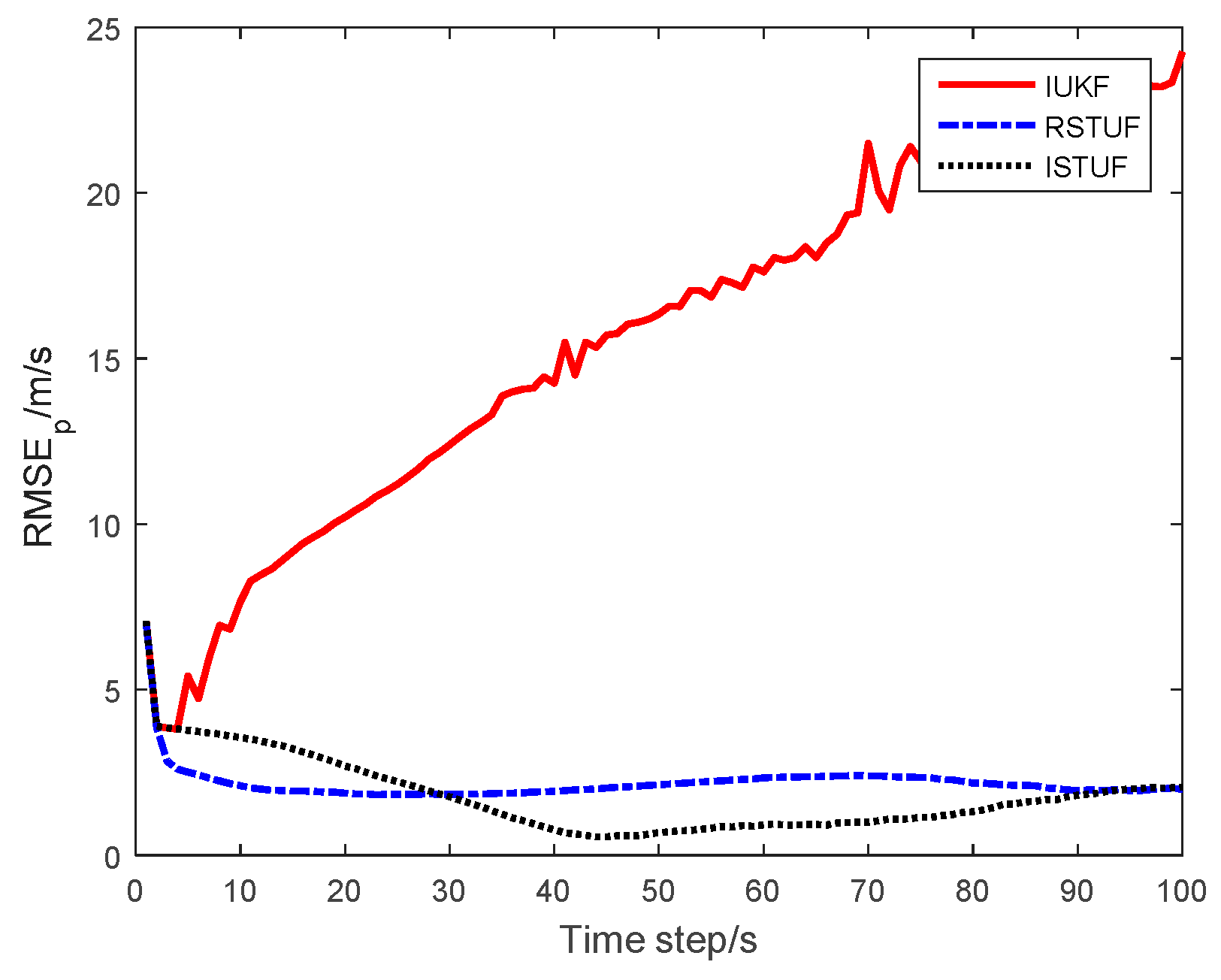
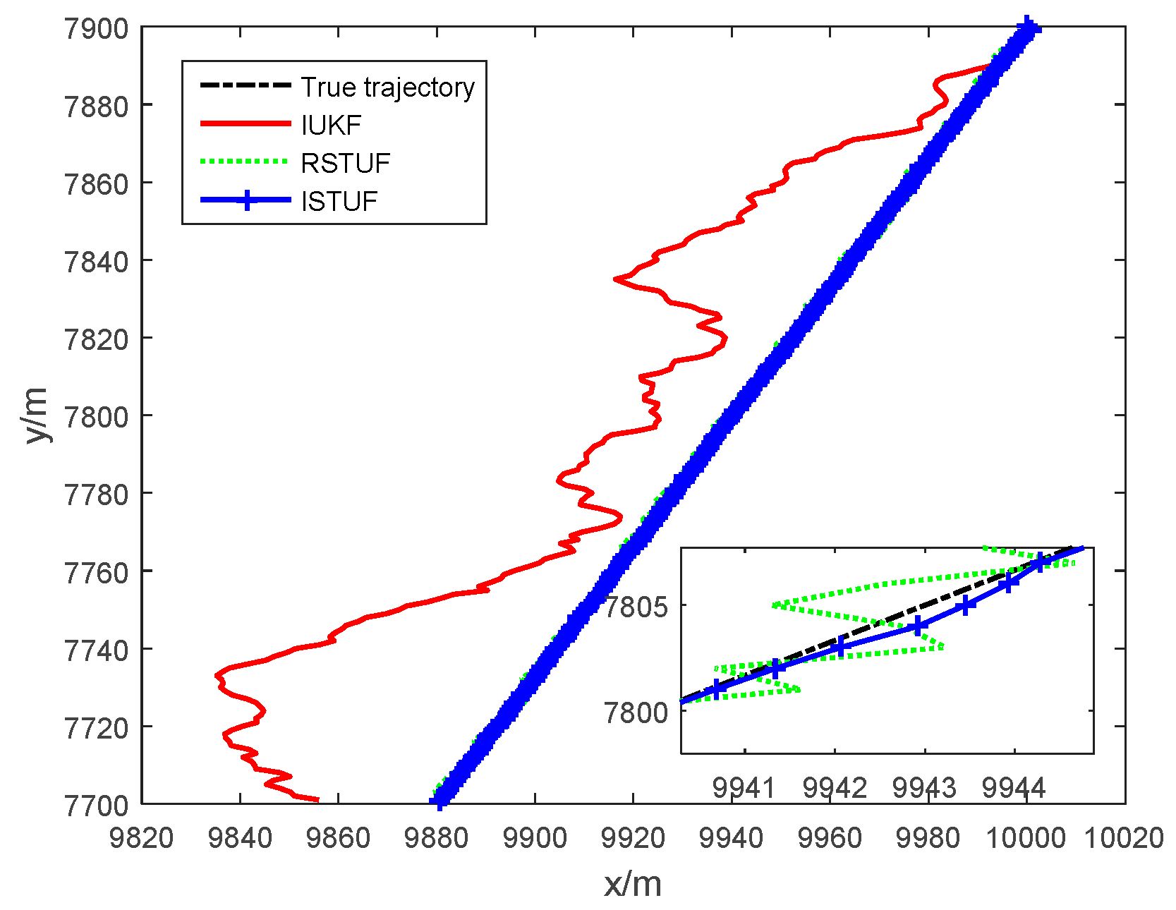
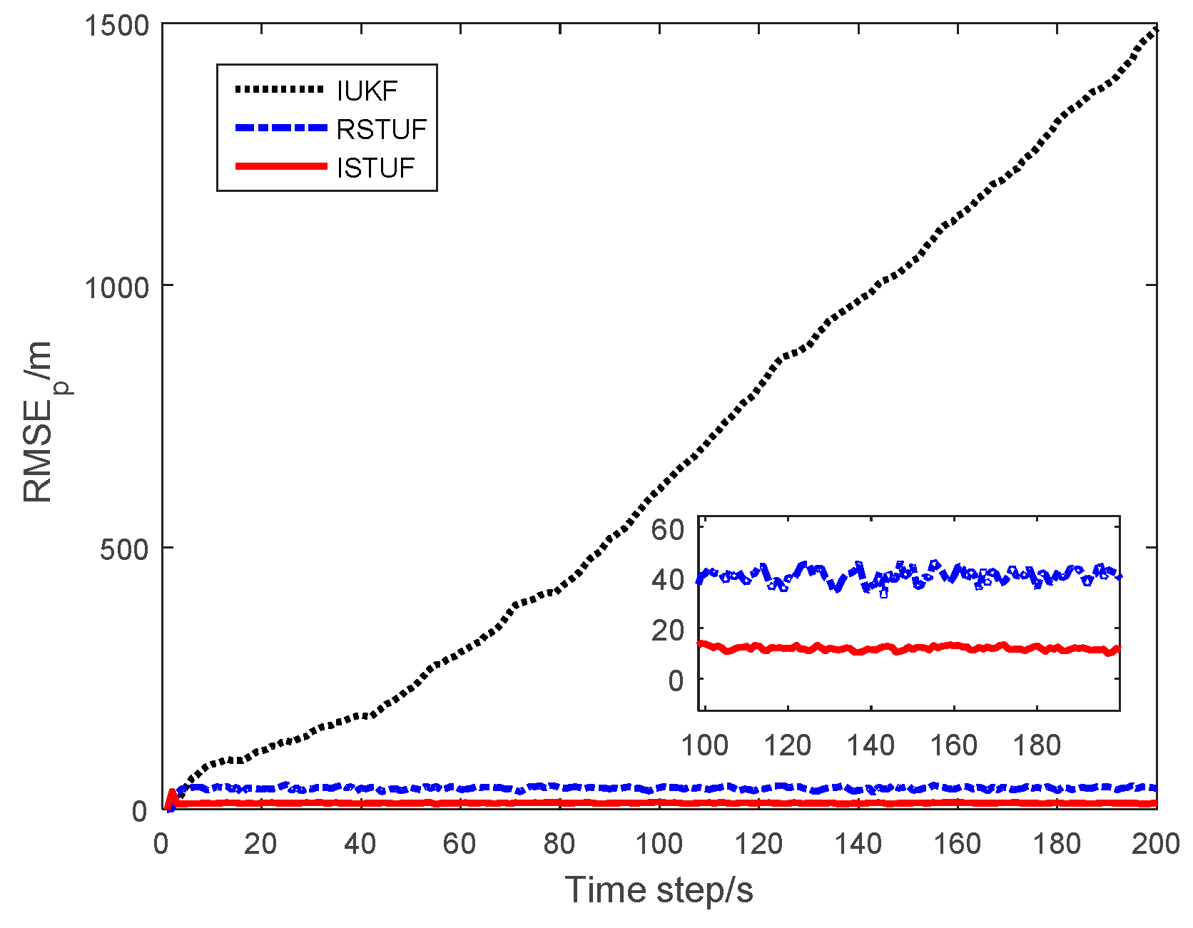
In case 2, the probability of γ k = 1 was set as p k = 0.4 , i.e., the probability of the time-delayed measurement increased. Moreover, the noises have been enlarged. The comparison between the true trajectory and estimated trajectories is shown in Figure 5, and it is clear that the estimated trajectory of ISTUF was closest to the real trajectory. The trajectory of IUKF has been divergent, because of the effect of heavy-tailed noise.
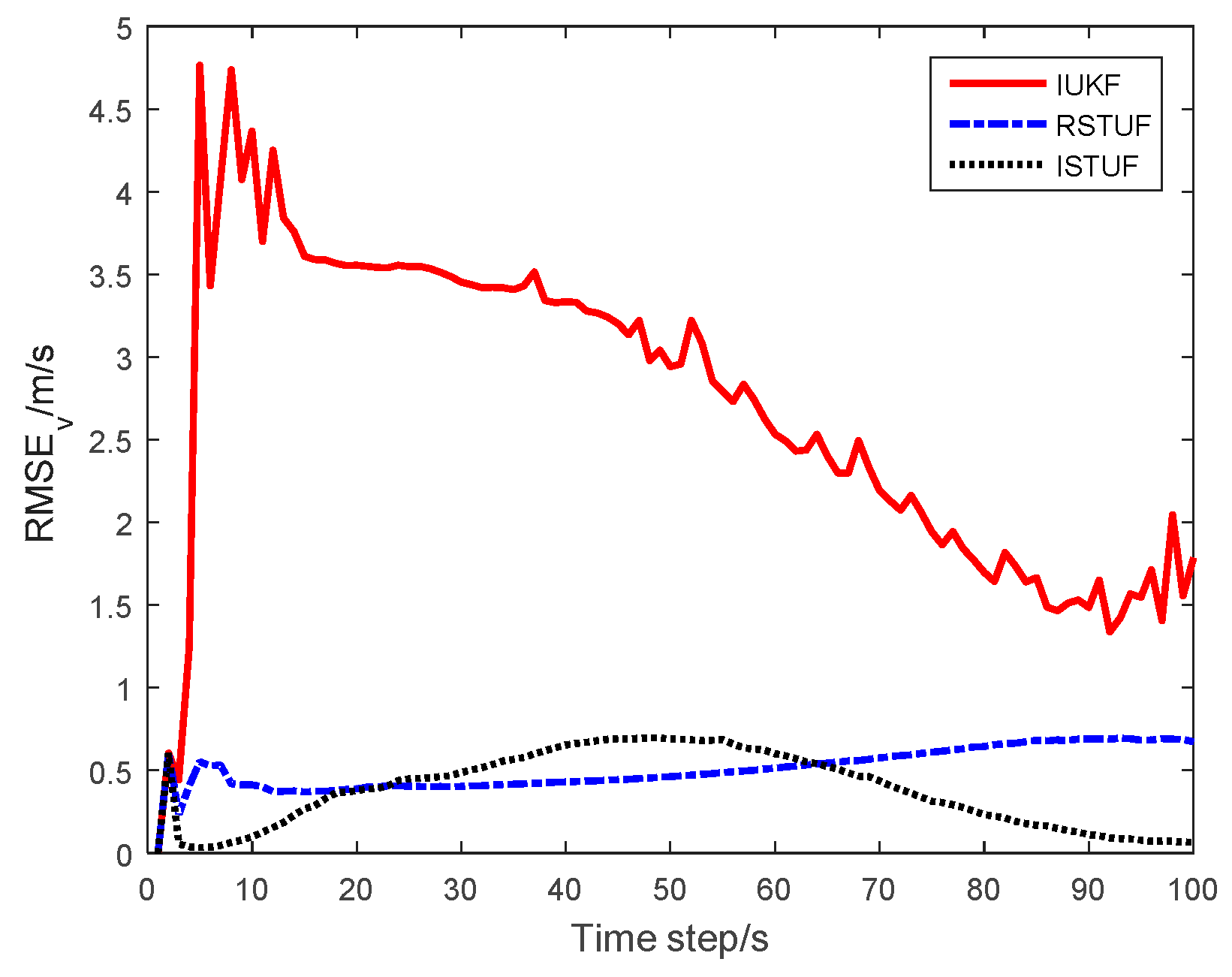
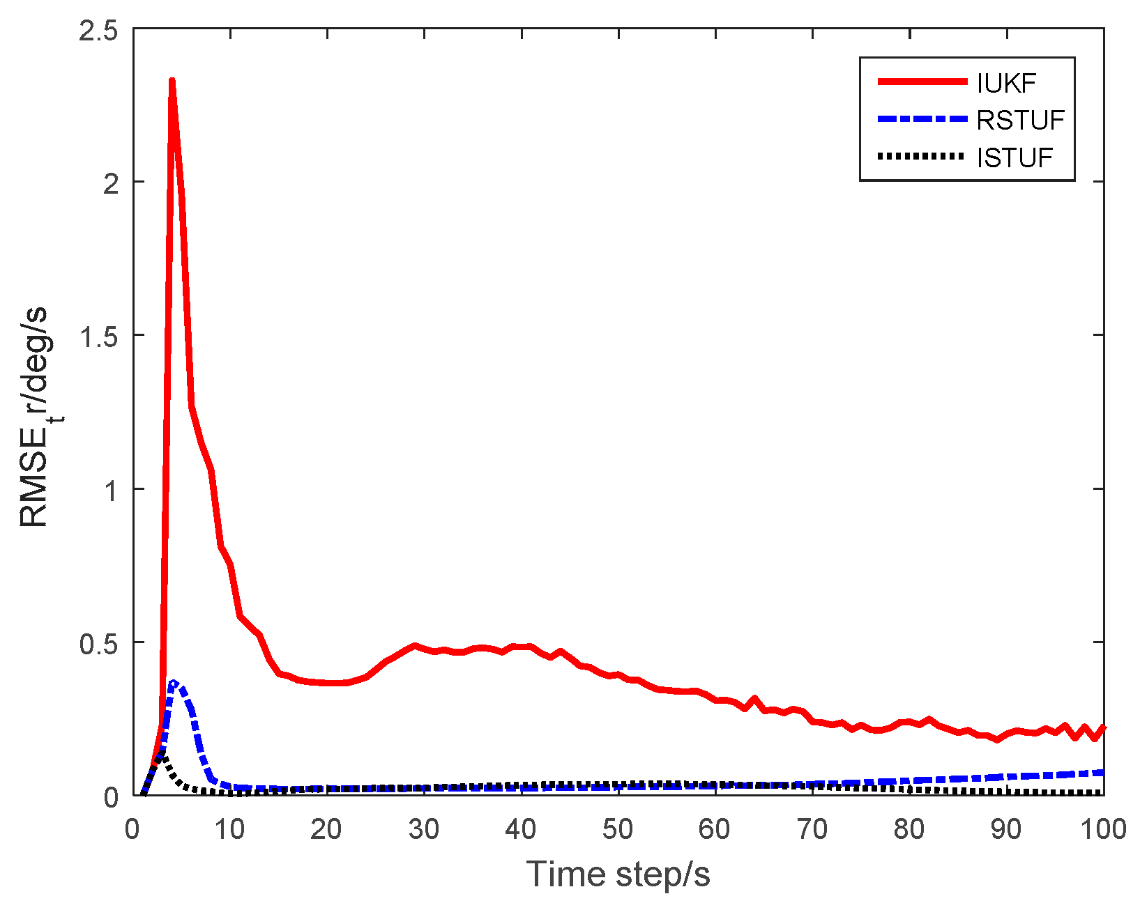
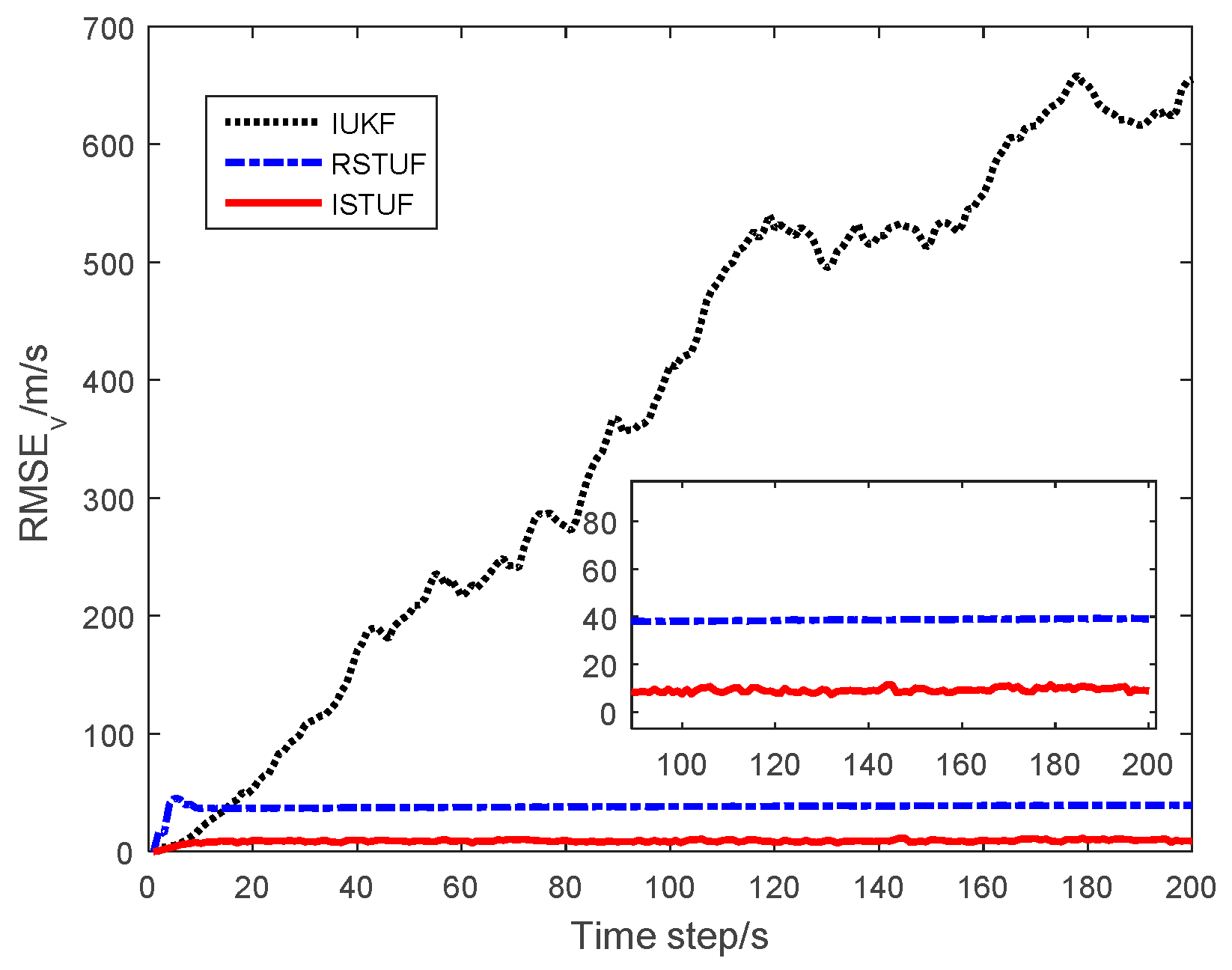
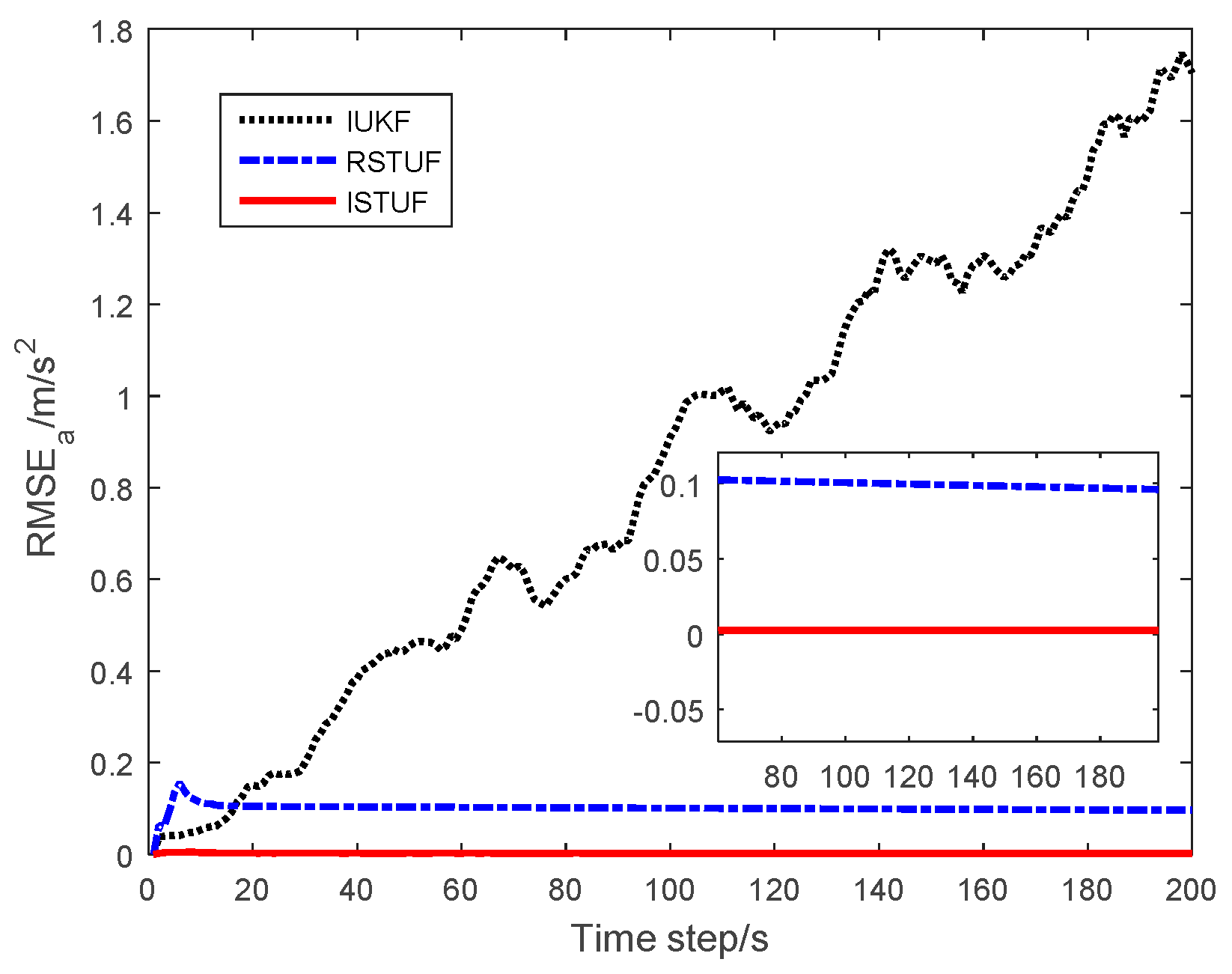
The RMSEs of the estimating results are shown in Figure 6, Figure 7 and Figure 8. The figures indicate that the RMSE of IUKF had been divergent, i.e., the enlarged heavy-tailed noise seriously affected the performance of filters under GF framework. The RMSE of RSTUF was also larger than that of ISTUF obviously. As the probability of time-delayed measurement had increased, the effect of the phenomenon was aggravated.
The ARMSE of the three filters is listed in Table 3. It is clear that the ARMSE of ISTUF was less than IUKF and RSTUF, and the ARMSE of IUKF was too large. As a result, ISTUF was more suitable for a target tracking system with time-delayed measurement and time-correlated heavy-tailed noises.

6. Conclusions

In the paper, a novel filter ISTUF has been designed for systems with one-step delayed measurement, and time-correlated heavy-tailed noises. The linear recursive model with STD was first used to construct the time-correlated heavy-tailed noises. Furthermore, augmenting the state with measurement noise can deal with the correlation problem caused by one-step delayed, and UT was applied to calculate the Student’s t weighted integral accurately. The simulation results illustrated that ISTUF reached a higher estimating accuracy than IUKF and RSTUF, and the computational cost of ISTUF is similar to IUKF and RSTUF.

Author Contributions

Conceptualization, X.W. and K.M.; methodology, X.W.; software, X.W.; validation, X.W.; formal analysis, X.W.; investigation, X.W.; resources, K.M.; data curation, X.W.; writing—original draft preparation, X.W.; writing—review and editing, K.M.; visualization, X.W.; supervision, K.M.; project administration, K.M.; funding acquisition, K.M.

Funding

This research received no external funding.

Conflicts of Interest

The authors declare no conflict of interest.

References

  1. Karlgaard, C.D.; Schaub, H. Huber-Based Divided Difference Filtering. J. Guid. Control Dyn. 2012, 30, 885–891. [Google Scholar] [CrossRef]
  2. Chang, L.; Hu, B.; Chang, G.; Li, A. Huber-based novel robust unscented Kalman filter. IET Sci. Meas. Technol. 2012, 6, 502–509. [Google Scholar] [CrossRef]
  3. Chien-Hao, T.; Lin, S.F.; Dah-Jing, J. Robust Huber-Based Cubature Kalman Filter for GPS Navigation Processing. J. Navig. 2016, 70, 527–546. [Google Scholar] [Green Version]
  4. Deng, Z.; Yin, L.; Huo, B.; Xia, Y. Adaptive Robust Unscented Kalman Filter via Fading Factor and Maximum Correntropy Criterion. Sensors 2018, 18, 2406. [Google Scholar] [CrossRef]
  5. Wang, Y.; Zheng, W.; Sun, S.; Li, L. Robust Information Filter Based on Maximum Correntropy Criterion. J. Guid. Control Dyn. 2016, 39, 1–6. [Google Scholar] [CrossRef]
  6. Chen, B.; Liu, X.; Zhao, H.; Principe, J.C. Maximum correntropy Kalman filter. Automatica 2017, 76, 70–77. [Google Scholar] [CrossRef] [Green Version]
  7. Huang, Y.; Zhang, Y.; Li, N.; Wu, Z.; Chambers, J.A. A novel Robust student’s t-based Kalman filter. IEEE Trans. Aerosp. Electron. Syst. 2017, 53, 1545–1554. [Google Scholar] [CrossRef]
  8. Gustafsson, F.; Gunnarsson, F.; Bergman, N.; Forssell, U.; Jansson, J.; Karlsson, R.; Nordlund, P.-J. Particle Filters for Positioning, Navigation and Tracking. IEEE Trans. Signal Process. 2002, 50, 425–437. [Google Scholar] [CrossRef]
  9. Míguez, J. Analysis of selection methods for cost-reference particle filtering with applications to maneuvering target tracking and dynamic optimization. Digit. Signal Process. 2007, 17, 787–807. [Google Scholar] [CrossRef]
  10. Zaitouny, A.; Stemler, T.; Algar, S.D. Optimal Shadowing Filter for a Positioning and Tracking Methodology with Limited Information. Sensors 2019, 19, 931. [Google Scholar] [CrossRef] [PubMed]
  11. Zaitouny, A.A.; Stemler, T.; Judd, K. Tracking Rigid Bodies Using Only Position Data: A Shadowing Filter Approach based on Newtonian Dynamics. Digit. Signal Process. 2017, 67, 81–90. [Google Scholar] [CrossRef]
  12. Judd, K. Tracking An Object with Unknown Accelerations Using A Shadowing Filter. arXiv 2015, arXiv:1502.07743. [Google Scholar]
  13. Huang, Y.; Zhang, Y.; Li, N.; Chambers, J. Robust Student’st based nonlinear filter and smoother. IEEE Trans. Aerosp. Electron. Syst. 2016, 52, 2586–2596. [Google Scholar] [CrossRef]
  14. Roth, M.; Özkan, E.; Gustafsson, F. A Student’s t filter for heavy tailed process and measurement noise. In Proceedings of the IEEE International Conference on Acoustics, Speech and Signal Processing, Brighton, UK, 12–17 May 2019; pp. 5770–5774. [Google Scholar]
  15. Huang, Y.; Zhang, Y. Robust student’s t-based stochastic cubature filter for nonlinear systems with heavy-tailed process and measurement noises. IEEE Access 2017, 5, 7964–7974. [Google Scholar] [CrossRef]
  16. Bryson, A.; Johansen, D. Linear filtering for time-varying systems using measurements containing colored noise. IEEE Trans. Autom. Control 1965, 10, 4–10. [Google Scholar] [CrossRef]
  17. Liu, W. State estimation of discrete-time systems with arbitrarily correlated noises. Int. J. Adapt. Control Signal Process. 2014, 28, 949–970. [Google Scholar] [CrossRef]
  18. Bryson, A., Jr.; Henrikson, L. Estimation using sampled data containing sequentially correlated noise. J. Spacecr. Rocket. 1968, 5, 662–665. [Google Scholar] [CrossRef]
  19. Petovello, M.G.; O’Keefe, K.; Lachapelle, G.; Cannon, M.E. Consideration of time-correlated errors in a Kalman filter applicable to GNSS. J. Geod. 2009, 83, 51–56. [Google Scholar] [CrossRef]
  20. Hermoso-Carazo, A.; Linares-Pérez, J. Unscented filtering algorithm using two-step randomly delayed observations in nonlinear systems. Appl. Math. Model. 2009, 33, 3705–3717. [Google Scholar] [CrossRef]
  21. Wang, X.; Liang, Y.; Pan, Q.; Zhao, C. Gaussian filter for nonlinear systems with one-step randomly delayed measurements. Automatica 2013, 49, 976–986. [Google Scholar] [CrossRef]
  22. Gu, Y.; Li, J.; Feng, D. State filtering and parameter estimation for linear systems with d-step state-delay. IET Signal Process. 2014, 8, 639–646. [Google Scholar] [CrossRef]
  23. Li, M.; Zhang, L.; Chu, D. Optimal Estimation for Systems with Multiplicative Noises, Random Delays and Multiple Packet Dropouts. IET Signal Process. 2016, 10, 880–887. [Google Scholar] [CrossRef]
  24. Geng, H.; Wang, Z.; Cheng, Y.; Alsaadi, F.E.; Dobaie, A.M. State estimation under non-Gaussian Lévy and time-correlated additive sensor noises: A modified Tobit Kalman filtering approach. Signal Process. 2019, 154, 120–128. [Google Scholar] [CrossRef]
  25. Ding, Z.; Liu, Y.; Liu, J.; Yu, K.; You, Y.; Jing, P.; He, Y. Adaptive Interacting Multiple Model Algorithm Based on Information-Weighted Consensus for Maneuvering Target Tracking. Sensors 2018, 18, 2012. [Google Scholar] [CrossRef]
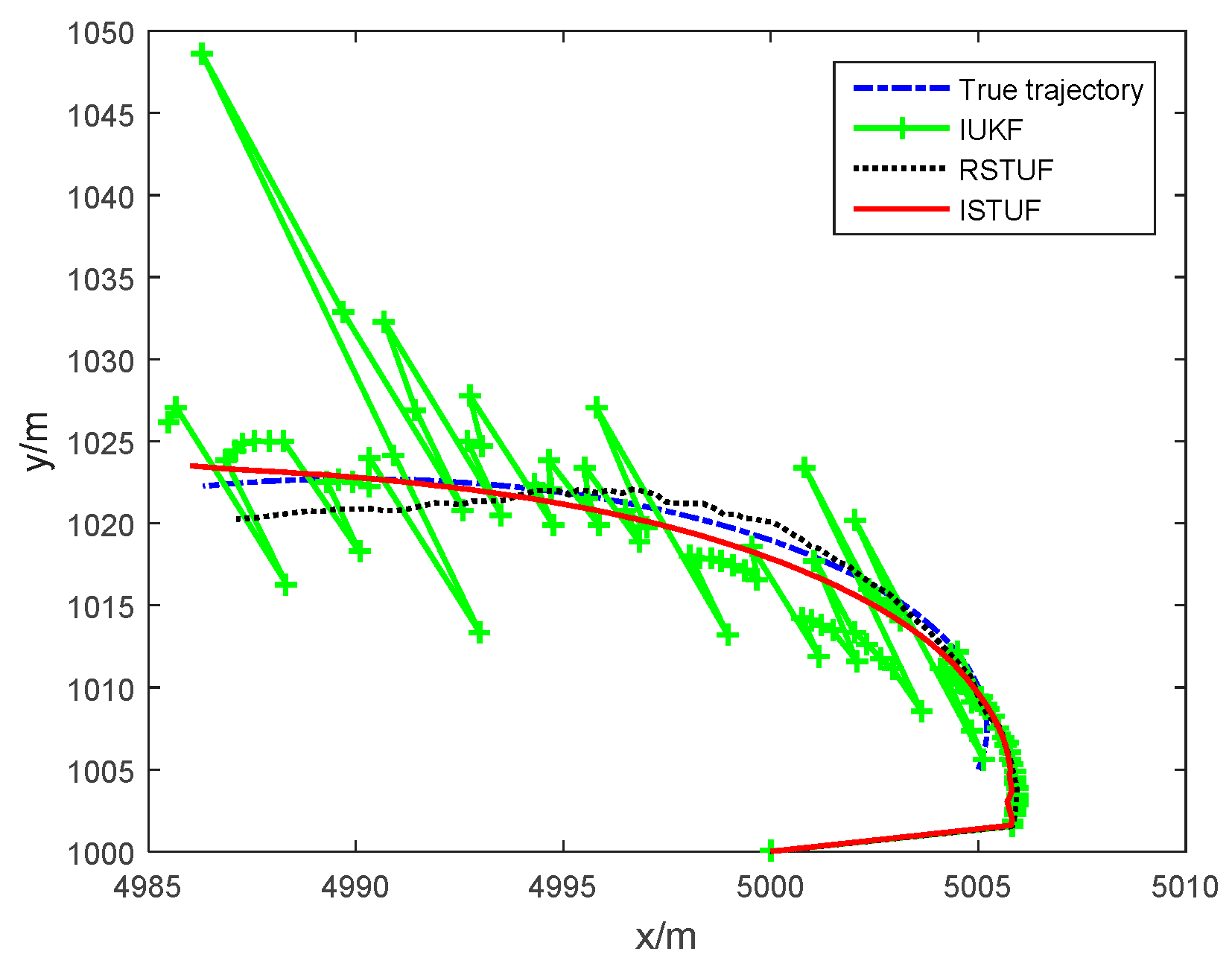
Figure 1. Comparison of the trajectories.
Applsci 09 02186 g001
Figure 2. RMSE of estimating position.
Applsci 09 02186 g002
Figure 3. RMSE of estimating velocity.
Applsci 09 02186 g003
Figure 4. RMSE of estimating turn rate.
Applsci 09 02186 g004
Figure 5. Comparison of the trajectories.
Applsci 09 02186 g005
Figure 6. RMSE of estimating position.
Applsci 09 02186 g006
Figure 7. RMSE of estimating velocity.
Applsci 09 02186 g007
Figure 8. RMSE of estimating acceleration.
Applsci 09 02186 g008
Table 1. The difference between improved Student’s t based unscented filter (ISTUF)and RSTUF.
ProblemsISTUFRSTUF
Dealing with STD noisesUse the Student’s t filtering frameworkUse the Student’s t filtering framework
Dealing with time-correlated noisesBased on measurement differencing method, rewrite the noise function to time-irrelevant form.no action
Dealing with the randomly delayed measurementExpand the state vector with measurement noise, and consider the conditional PDF of the measurement noise.no action
Calculating the Student’s t weighted integralsUse the UT methodUse the UT method
Table 2. The ARMSE and time consuming of the three filters.
FiltersARMSE of PositionARMSE of VelocityARMSE of Turn RateTime Consuming
IUKF14.779 m2.866 m/s0.607°/s0.0481 s
RSTUF2.342 m0.578 m/s0.051°/s0.0494 s
ISTUF1.841 m0.386 m/s0.027°/s0.0519 s
Table 3. The ARMSE of the three filters.
FiltersARMSE of Position
(m)
ARMSE of Velocity
(m/s)
ARMSE of Acceleration
(m/s2)
IUKF662.2783327.11310. 9213
RSTUF40.788737.77530.0748
ISTUF12.11378.82900.0247