SPL Features Quantification and Selection Based on Multiple Multi-Level Objectives

Abstract

Software Product Lines (SPLs) can aid modern ecosystems by rapidly developing large-scale software applications. SPLs produce new software products by combining existing components that are considered as features. Selection of features is challenging due to the large number of competing candidate features to choose from, with different properties, contributing towards different objectives. It is also a critical part of SPLs as they have a direct impact on the properties of the product. There have been a number of attempts to automate the selection of features. However, they offer limited flexibility in terms of specifying objectives and quantifying datasets based on these objectives, so they can be used by various selection algorithms. In this research we introduce a novel feature selection approach that supports multiple multi-level user defined objectives. A novel feature quantification method using twenty operators, capable of treating text-based and numeric values and three selection algorithms called Falcon, Jaguar, and Snail are introduced. Falcon and Jaguar are based on greedy algorithm while Snail is a variation of exhaustive search algorithm. With an increase in 4% execution time, Jaguar performed 6% and 8% better than Falcon in terms of added value and the number of features selected.

1. Introduction

Modern ecosystems demand rapid development of large-scale software. There are many approaches such as Model Driven Development (MDD), component development, Commercial Off The Shelf (COTS), and Software Product Lines (SPLs). However, SPLs maintain a significant share among leading organizations. SPLs are heavily dependent on the selection of features, based on the business goals and objectives. In most industries, there are thousands of candidate features that can potentially participate in a given product. Each of them has its own advantages and disadvantages over the other. Selecting these features manually while taking into account the business objectives and constraints can be challenging. There have been a number of attempts to automate the feature selection, however, they had limited success due to their limited capabilities in terms of number of supported objectives and customization. Addressing these issues is significant as their current form cannot be applied. This is due to lack of means of quantifying datasets and automatically selecting the features based on custom made complex rules and objectives. This research aims to address the above issues by proposing:

• A novel way for quantifying feature properties based on business goals and objectives. The proposed approach can quantify datasets containing features belonging to different categories with numeric and text-based property values using twenty operators. Additionally, it calculates a metric called added value (see Section 3.4). The summary of the added value of all features participating in the product is called product added value and it is used to determine the fitness of the product.
• Three multi-level multi-objective feature selection algorithms called Falcon, Jaguar, and Snail which are compatible with proposed quantification process. The first two are based on greedy algorithm, while the third is a variant of exhaustive search. The algorithms automatically select features based on multivalued objectives, which are set at feature, category or product levels (see Section 4).

The proposed approach is novel in many aspects such as; it takes a holistic approach by providing an integrated methodology that starts from the specification of the business goals and objectives, leading to the quantification of features and generation of the product profile along with its meta data. Our proposed approach quantifies the features based on customizable user-defined objectives and calculates their added value (fitness score). It then automatically selects one of the three included selection algorithms (or allow the user to pick one) based on the dataset and auto-complete the product profile, while it ensures that no user defined constraints have been violated. Figure 1 shows an overview of the proposed approach.

As can be seen in Figure 1, the process of product profile generation starts with the creation of SPL and product/s for that SPL. The user must define objectives at features property level for data quantification. The data quantification uses the operators as shown in the two tables in the diagram for strings and numeric data. The user must set product level objectives, in order for the selection algorithms to produce a product profile. The features quantification, results in added value for the properties based on the importance level set by the user. The list of quantified features is sorted based on added value.

An original dataset with 46K+ features, extracted from Unity3D assets store, was used for demonstrating and evaluating the proposed approach. A software tool called Feature Selection Engine (FSE) developed as part of this research, was used for implementing and testing the proposed approach. The results showed that Snail can only be used for small datasets, while Falcon is best suited for large datasets. Jaguar performed better in terms of product added value, in large dataset that contain product property level objectives.

The next section presents the literature review, where the state of art of data quantification and feature selection algorithms is presented. Section 3 and Section 4 introduce the proposed feature’s quantification approach and the three selection algorithms. Section 5 presents the FSE. Section 6 discusses the performance of the three algorithms in different scenarios with different datasets based on the results of the FSE. Section 7 concludes this work, states its limitations, and proposes some future work.

2. Literature Review

Feature selection, studied in the literature, is based on two important aspects: functional and non-functional requirements. Meeting all the requirements might be an issue due to many factors including that of quantification of various elements that are without clear quantitative constraints. Also, the trade-off between different quantities which vary in their ranges, have issues with feature selection [1]. Quantification of features as well as constraints have been studied in the recent literatures. Constraints or non-functional requirements are represented as binary size or performance or total budget, which are numeric in nature and thus making the features qualified initially [2].

Qualitative and quantitative features are considered [3]: qualitative features are represented using a qualifier tag in an ordinal scale; meanwhile, quantitative features are represented as numerical values. Features are represented either as integers [4] or binary [5] values. The authors in [4] represented features as a value or a binary string, as stated in Equation (1):

$$F=\left\{f_i\right\},1\le i\le n$$

$$\begin{array}{c}V\left(f_i\right)=thevalueof{f}_i\\ R\left(f_i\right)=theresourceconsumedby{f}_i\\ \begin{array}{c}{R}_c\subset theresourceconstraints\\ S=abinarystringwithnbits\end{array}\end{array}$$

(1)

Features are compared using Jaccard distance to decide which of them are to be selected. In order to apply Jaccard distance, quantification of the required features is necessary [6]. Combining constraint solving and searching is performed using diversity performance and search using smart operators. Feature clustering [7] based on groups is also used for quantification.

Earlier feature selection algorithms such as SAT Solver (SATISFIABILITY solver), CSP (Constraints Satisfaction Problem), and BDD (Binary Decision Diagrams) did not consider resource constraints. Guo et al. [2] used genetic algorithm, named as GAFES (Genetic Algorithm for FEature Selection), to tackle the problem of feature selection optimization with resource constraints. Filtered Cartesian Flattering (FCF) is used for evaluation purposes by changing SPL Feature selection into Multi-dimensional Multiple-choice Knapsack Problem (MMKP) using two kinds of optimization techniques i.e., Branch and Bound with Linear Programming (BBLP) [8] to find an exact solution and Modified HEUristic (M-HEU) [9] to handle upper and lower bounds. A random feature selection was transmuted into a valid feature grouping that conforms to the constraints of the feature model and improved the search process to speed up the discovery of features selection. The experimental results showed that FCF + M-HEU optimality was better at time-saving than GAFE by about 8% to 9% while GAFE was only found to be less time-consuming than the other two combinations. Optimality of GAFE solution remained relatively stable at 86% as the other techniques used had exponential time complexity. Overall, all heuristic methods have polynomial algorithmic complexity.

Lin et al. [4] describe the software product derivation as feature selections with resource constraints but they define it as an NP-hard problem. Lin et al. [4] modified ACO (Ant Colony Optimization algorithm) to have cross tree constraint, if the next selection of feature is to be considered. For the experiment, they used the dataset from SPLOT tool repository of feature model (using the feature model of E-SHOP).

Bosch et al. [10] proposed FESPA (Feature Extraction and Selection for Predictive Analytics) for the feature generation and selection. The proposed model is applied using EXPLOREKIT, which is an existing implementation of feature generation and selection. FESPA works in two phases: feature generation and feature selection. Feature selection is done through background classifier which is based on meta features (belonging to one or more categories). Meta features are calculated for each feature, and then a decision tree is used and trained on all meta features and stored in a file.

In

Table 1. Algorithms for feature selection. GAFES: Genetic Algorithm for FEature Selection; FCF: Filtered Cartesian Flattering; BBLP: Branch and Bound with Linear Programming; M-HEU: Modified HEUristic.

#	Paper	Algorithm used	Algorithms used for comparison/validation	Results
1.	A genetic algorithm for optimized feature selection with resource constraints in SPL	GAFES (2011)	FCF + BBLP FCF + M-HEU	Time consumption in larger data set GAFES has an advantage while in small data set the competitors had the advantage
2.	Ant colony optimization for feature selection in SPL	Ant colony optimization (GA-ACO algorithm)	FCF + M-HEU GAFES	6% worse running time than FCF+M-HEU 10% better but taking more time
3.	Automatic feature generation and selection in predictive analytics solutions	-FESPA -Decision tree -Explore kit for feature selection		Besides feature generation and feature selection, Data cleaning is also an important part of the data pre-processing phase but is out of the scope of this research.

, we summarize the core contributions and the methods used by the authors of the above articles:

Sayyad et al. [11] complementing the work of Guo et al. [2] showed the superiority of IBEA over NSGA-2 and SPEA 2 in searching complex structures with many objectives (multiple objectives) through multiple graphs using five hours experiment using the hyper volume indicator, the spread and percentage of correct indicator.

Henard et al. [6] modified the original IBEA algorithm to SATIBEA based on MOO (Multi-Objective Optimization) with multiple objectives search-based optimization with constraints, for feature selection. It was based on five objectives: correctness, the richness of features, used before features, known defects, and cost. The work is mainly focused on handling constraints as the previous work of Sayyad et al. [11] have not explicitly included any techniques. SATIBEA works by incorporating two smart search operators, smart mutation and smart replacement operators, along with constraints solving.

Lian et al. [1] complement the work of Sayyad et al. [11] by accepting IBEA, which outclasses the generally-used MOEAs and adopts their fitness function in their experimentation for features selection mechanism. The tests performed using IVEA algorithm was compared with IBEA, NSGA 2, and SPEA2 algorithms. The results showed the supremacy of IVEA over the other on NFR Optimization in terms of execution time.

Xue et al. [12] improved the IBEA algorithm for MOEAs by adding Differential Evaluation (DE) as IBEA is believed to be underperforming in finding diverse and correct solutions. The combination proposed is to address the issue of product configuration in such a way that to find features that have zero conflicts and at the same time try to achieve the MOEAs by reducing the cost and increasing the number of features. IBED is a combination of IBEA and DE, which incorporates feedback mechanism for finding correct solutions.

Neto et al. [13] suggested a method called Product Portfolio Scoping (PPS), which is a marketing-based approach focusing on how features of a product should be developed by emphasizing on cost reduction and customer satisfaction by categorizing it as an NP-hard problem. They used a hybrid algorithm approach to combine NSGA 2 and Mamdani FUZZY inference system. The binary objectives tested in the approach were cost and relevance of features for each customer segment. The validation of the work was done by asking the practitioners who were interviewed for the configuration of the fuzzy systems. They suggested as future work that they have not dealt with a large number of a feature on the configuration of stage-2. In addition, the synthetic SPL (with no real asset) was used and the approach was not tested on a large number of features.

Ferreira et al. [14] proposed H-H (Hyper Heuristics) approach to select dynamically the best operator in SPL for testing, as the increasing size and complexity of application can make product line testing impossible. They considered four objectives to the problem, which include product quantity, mutation score, pair wise coverage and dissimilarity of products. A hyper heuristic is automatic selection or generation of heuristics for solving a complex problem. The hyper heuristic model was used with 4 MOEAS namely NSGA 2, IBEA, SPEA2, and MOEA/D-DRA incorporating 2 selection methods, random and Upper Confidence Bound (UCB). It was found that NSGA 2-H-H was better and dominant over NSGA 2 for large instances, while for small instances random selection was acceptable.

Lian et al. [15] proposed a new algorithm by the name of IVEA-2 to solve the problem of product customization in SPL with multiple objectives. Five objectives in this case study were considered (correctness, reuse, less error, lower cost, and more features) so that an optimal solution between competing and conflicting objectives is taken into consideration. They used the same dataset used by Sayyad et al. [11]. The results were tested against IBEA and SATIBEA algorithms and the results show that IVEA-2 outperforms on the effectiveness of producing the optimal valid solutions for large-scale feature models over a set period of time, having better diversity and convergence.

Table 2. Comparison of MOO (Multi-Objective Optimization) Algorithms.

#	Paper	# of Objectives Tested	Algorithm Used	Algorithms Used for Comparison/Validation	Results
1	Optimum feature selection in software product lines: Let your model and values guide your search	3	IBEA	NSGA-2 and SPEA-2	IBEA in searching complex structures with many objectives has a clear advantage over others.
2	Combining Multi-Objective Search and Constraint Solving for Configuring Large Software Product Lines	5	SATIBEA	IBEA Filtered (F)	SATIBEA is better in providing a quick stabilized solution
3	Optimized feature selection towards functional and nonfunctional requirements in software product lines.	0	IVEA	IBEA NSGA-2 SPEA = 2	IVEA has better performance in four factors Spread, HV, IGD and EPSLILON
4	IBED: Combining IBEA and DE for optimal feature selection in SPLE	2	IBED	IBEA NSGA 2 ssNSGA 2 MOCell	Correctness and diversity of the found solutions. Reduced the time in finding a solution by 30–40 s.
5	Binary Multi-objective PSO and GA for Adding New Features into an Existing Product Line	2	Pso AND NSGA 2	Compared between their self	Adding new features into the existing product line. GA performs better than PSO
6	A hybrid approach to suggest SPL Portfolios	2	Mamdani Fuzzy inference system (a hybrid of all algorithm and not dependent on an algorithm)	Random search algorithm (sanity check)	The hybrid approach is much better than random search algorithm in terms of suitability and hypervolume values attached, while the time spent is the same.
7	Hyper-Heuristic based product selection for SPL	4	Nsga-2, SPEA 2, IBEA and MOEA/D-DRA	Comparative analysis among all of them	NSGA-2 generates the best results
8	An approach for optimized Feature selection in large-scale software product lines	5	IVEA 2	SATIBEA IBEA	IVEA-II can generate more valid solutions over a set period of time, with optimal solutions also having better diversity and convergence

summarizes the MOO algorithms and their effectiveness based on different sets of objectives.

This section presented a state-of-the-art literary review on feature quantification and selection algorithms. The current approaches do not support feature selection based on multiple multi-level objectives. In the proposed approach, objectives can be set at product/category and property level. Also, they do not propose an enriched quantifying text-based feature properties. The following section introduces our work.

3. Features Quantification

3.1. Introduction

In this research, we quantify features by quantifying their property values. To this end, we designed an approach that allow users to define 20 different type of objectives for quantifying feature property values (one per property at a given time). The features level objectives will be used to quantify the values of the corresponding properties and contribute to the Feature’s added value calculation of the product. The quantification of features and the selection algorithms are driven by user-defined constraints and objectives. Constraints are intended goals that must be achieved for the product in order to be qualified, while objectives are achievements that can be quantified in a fuzzy way and effect the value of the product. Constraints and objectives can be both applied to product/category level and/or the feature’s level property values. Feature property value objectives are used for feature quantification while product/category objectives are used for feature selection. The quantification of the different feature properties is described in the following sections.

3.2. Quantification of Text Based Properties

In this research, we implemented eight operators that allow users to quantify properties with text-based values. These operators and their results are presented in

Table 3. Operators used for finding Strings/Text for the selection of Features.

Operator	Type	Result
		If Keywords [Array] = Strings (Dataset)	Else
Include Strings	Fuzzy	100%	Strings found/total number of strings looking for * 100
Exclude Strings	Fuzzy	0%	100% to 1%
Include AND Exclude	Fuzzy	100% for Inclusion and 0% for Exclusion Return average	1% to 99% based on average Return average
Must Include	Boolean	If all strings are matched, 100%	Else 0%
Must Not Include	Boolean	0%	100%
Must Include AND Must Exclude	Boolean	100% and 0% Return average	0% and 100% Return average
Must Include AND Exclude	Fuzzy	100% and 0% Return average	0%–99% and 100–1% Return average
Include AND Must Exclude	Fuzzy	100% (Include) and 0% (Must Exclude) Return average	0%–99% (Include) and 100% (Must Exclude) Return average

. Fuzzy operators return a value from 0 to 100, while Boolean returns either 0 or 100.

As shown in Table 3, Boolean types return either 0% or 100%. The result of fuzzy types vary from 0% to 100% based on the what is matched and what is not. This also considers strings that ought to be included and those which ought to be excluded. Equation (2), used for “Include strings”, shows the calculation of Quantified Property Value (QPV), which is based on the ratio of number of strings matched to the number of strings to be matched.

$$\begin{array}{c}\begin{array}{c}QPV=\left(\frac{NS{M}^{\prime }}{NSM}\ast 100\right)\\ {Where,NSM}^{’}isthenumberofstringsmatched\end{array}\\ NSMisthenumberofstringstobematched\end{array}$$

(2)

The operator “Exclude strings” also uses Equation (2) replaced with strings not to be matched instead of strings to be matched. The operator “Include AND Exclude” is the average value of “Include” and “Exclude”. The operators with “Must” emphasizes the match or mismatch of all the given strings for “Include” and “Exclude” respectively. The operators with mix of “Must” and Fuzzy, will be calculated as: If the Boolean condition is True, the Fuzzy value will be calculated; Else, 0% will be returned as the Boolean is False.

3.3. Quantification of Numeric Properties

Numeric properties can be quantified based on the operators presented in

Table 4. Operators used for quantifying numeric property values.

Operator	Type	Operator	Type
Equal to	Boolean	Approximately equal to	Fuzzy
Not Equal	Boolean	Upto (Higher Better)	Fuzzy
Upto (Lower Better)	Fuzzy	More than	Boolean
Less than	Boolean	Between	Boolean
Between (Higher better)	Fuzzy	Between (Lower better)	Fuzzy
Equal and Above (Higher better)	Fuzzy	Equal and Above (Lower better)	Fuzzy

.

Boolean operators represented in Table 4 return either 0% or 100% based on the condition. For the fuzzy operators, the output varies between 0% and 100% based on certain elements. For each property P, the minimum and maximum values are represented as $mi{n}_P$ and $ma{x}_P$. The operations provided maps the input property value from the dataset, $v_i$, of P to the output value, $v_i^{\prime }$. The target value for the given property P is $t_p$. In certain scenarios like between, there are two target values that indicates the top and bottom range values, represented as $t_p^1$ and $t_p^2$. The similarities present in the fuzzy operators are grouped into a procedure called “Proximity Calculation”, which is invoked with suitable parameters. The label “Lower-Better” indicates that properties with values close to the lower limit will be given higher scores. For example, in case of Upto (Lower-Better), while values up to the target value will be accepted with a score, the lower the property value, the higher the score would be. The label “Higher-Better” works in a similar way but higher property value will result to higher score.

For proximity calculation, we use the following inputs and formulas. The direction is represented as forward or backward. The faraway value used in the algorithm represents the minimum or maximum value of the property in the dataset. When the maximum property value is used, the backward direction is considered; for minimum property value, the forward direction is considered.

• Tget value: $t_p$
• Property value: $v_i$
• Faraway value: $F_v\in \left\{mi{n}_p,ma{x}_p\right\}$
• Better (High or Low): $Bϵ\left\{h|l\right\}$
• Direction (Forward or Backward): $Dϵ\left\{f|b\right\}$

Input parameters in order: (Faraway value, Target value, Property value, Better, Direction)

• Calculate the range value: $r=\left|F_v\right|+\left|t_p\right|$
• With Higher-Better and Backward:

  $$v_i^{\prime }=100-\left(\frac{\left|F_v\right|-\left|v_i\right|}{\left|F_v\right|-\left|t_p\right|}\ast 100\right)if\left(B=h\right){\displaystyle \cup }\left(D=b\right)$$
• With Higher-Better and Forward:

  $$v_i^{\prime }=\frac{\left|v_i\right|+\left|F_v\right|}{r}\ast 100if\left(B=h\right){\displaystyle \cup }\left(D=f\right)$$
• With Lower-Better and Backward:

  $$v_i^{\prime }=\frac{\left|F_v\right|-\left|v_i\right|}{\left|F_v\right|-\left|t_p\right|}\ast 100if\left(B=l\right){\displaystyle \cup }\left(D=b\right)$$
• With Lower-Better and Forward:

  $$v_i^{\prime }=\frac{\left|F_v\right|-\left|v_i\right|}{\left|F_v\right|-\left|t_p\right|}\ast 100if\left(B=l\right){\displaystyle \cup }\left(D=b\right)$$

The fuzzy operator “Approximately equal to” is calculated based on Equation (3):

$$v_i^{\prime }=\frac{\left|mi{n}_p-v_i\right|}{ma{x}_p-t_p}\ast 100$$

(3)

As shown in

Table 5. Proximity based formulas.

Quantification Procedure	Procedure Call
Equal and Above (Higher Better)	Proximity ($ma{x}_p$, $t_p$, $v_i$, $h$, $b$)
Equal and Above (Lower Better)	Proximity ($ma{x}_p$, $t_p$, $v_i$, $l$, $b$)
Between (Higher Better)	$Proximity\left(ma{x}_p,t_p,v_i,h,b\right)When{v}_i>t_p^1$ $Proximity\left(mi{n}_p,t_p,v_i,h,f\right)When{v}_i<t_p$
Between (Lower Better)	$Proximity\left(ma{x}_p,t_p,v_i,l,b\right)When{v}_i>t_p^1$ $Proximity\left(mi{n}_p,t_p,v_i,l,f\right)When{v}_i<t_p^2$
Upto (Higher Better)	Proximity ($mi{n}_p$, $t_p$, $v_i$, $h$, $f$)
Upto (Lower Better)	Proximity ($mi{n}_p$, $t_p$, $v_i$, $l$, $f$)

, based on the condition whether a higher or lower value is given higher preference and the operator, suitable quantification process is performed. For example, Upto (Higher-Better) invokes the proximity procedure with the minimum property value as the faraway value, higher to represent higher-better, forward as direction, along with the target value and the property value. This would calculate the output value by using the ratio of sum of property value and minimum property value to the sum of target value and minimum property value.

As an example with “Upto (Higher Better)”, for the Target Value Cost Upto (Higher Better) to “97”. The minimum value of this property is 1 and the maximum is 100, as shown in

Table 6. Example of values returned by Feature Selection Engine (FSE) for “Upto (Higher Better)”.

Feature	Value	FSE Generated Results
Cost of Feature 1	10	10.30
Cost of Feature 2	97	100
Cost of Feature 3	1	1.03
Cost of Feature 4	100	0

.

3.4. Calculation of the Feature Added Value

The added value of a feature ($O^{\prime }$) is the product of the Feature’s Category Importance (FCI) and the summation of the products of the Scores of the Quantified properties (SQp) and Importance (Io) (see Section 4.1) of the corresponding objectives. The algorithm allows the user to give priority to features that exist in another product of the same SPL, by adding a bias value (b) of 0.1 to the total score of the feature.

$$O^{\prime }=FCI\ast {\displaystyle \sum }SQp\ast Io+b$$

(4)

For each Objective “O”, the Importance Level values are represented as Multipliers “Low = 0.25, Medium = 0.5, High = 0.75, and Critical = 1.0”.

One exception to the above is when the quantified property score is 0 and the importance of the corresponding objective is Critical (4). In that case, the added value of the feature is set to −1. This exception ensures that features that do not meet critical objectives are disqualified. For example, if we are looking for 3D models, we set the objective that the sub-string “3D” should exist in the property “model type”. Then if the score of the quantified “model type” property is 0, it means that this is not a 3D model, hence this feature should be disqualified irrespective of the rest of its properties.

4. Feature Selection Algorithms

4.1. Product/Category Objectives

Feature selection algorithms are driven by objectives set at the product and/or category level. These objectives have a direct impact over the behavior of the selection algorithms.

4.1.1. Product Level Objectives

At the product level, our feature selection algorithms support the condition of minimum and/or maximum total number of features.

The default values set for the minimum number of features is zero and the maximum number of features to infinite. The minimum number of features has to be less or equal to the maximum number of features and both of them cannot be negative.

Moreover, the user can set/define constraints on the summary value of the feature’s numeric properties. These constraints include “less than”, “more than”, for example, the total cost of the product should be “less than” an “X” amount.

4.1.2. Category Level Objectives

At the Category level, the algorithms support minimum and maximum number of features similar to the product level but for a specific category. Additionally, we support maximum number of occurrences of the same features, which means how many times the same feature can appear in a given category, by default each feature can appear only once.

Furthermore, the user can specify the importance level of each category to “not important”, “low”, “medium”, “high”, and “very high”. This will affect the ranking of the features under this category, as elaborated in Section 4.4. Similar to product level, user can define constraints on the total value of the feature’s numeric properties. For example, the total cost for the category “3D models” should be “less than” an “X” amount.

4.2. Falcon Selection Algorithm

The Falcon selection algorithm, is a variant of the greedy algorithmic family, takes an input the list of quantified features, sorted by added value, and product/category level objectives. Initially, the algorithm will attempt to satisfy the objective (if present) that requires each product category to contain a minimum number of features. This is achieved by first attempting to add the features that belong to these categories. In more detail, for each category with a minimum number of features requirement, the algorithm traverses through the sorted list, identify the features of the same category, and attempt to add them to the product. The algorithm validates using the constraint violation approach, described below.

• The added value of the feature must be positive.
• The number of features under the product’s category must be less than the maximum number of features for this category.
• The number of occurrences of the feature in the product must be less than the maximum permitted.

Additionally, the following product/category property objectives are checked for each numeric quantified property.

4.

The total value of all features currently participating in the product and category for this property is less than the defined value.

After the algorithm ensures that each category has the minimum number of features required by the user-defined category objectives, it will attempt to satisfy (if required) the total property value of a product and/or category to be more than a certain value. To attempt this, the algorithm will sort the features based on maximum property value, giving priority to features with high property values. It will then attempt to add them to the product one-by-one until the constraint is validated. Upon completion of this task, it will attempt to add more features in order to increase the value of the product. The algorithm will traverse through the sorted list, adding all the features that do not violate any constrain. This is achieved by reusing the constrain violation mechanism described above. The above algorithm is illustrated in the Figure 2.

Falcon is guaranteed to execute in minimum time, but it is not guaranteed to produce a product with the best combination of features or even to produce a product due to the known limitations of the greedy algorithms. For example, the algorithm may fall in a dead-end due to miss-selection of features that have higher value but prevent other features with less individual added value, causing higher combined added value to be selected.

4.3. Jaguar Selection Algorithm

Jaguar works identical to Falcon, but with an extra step at the beginning. Instead of using the list of candidate features sorted by added value, it re-sorts the list based on an Added Value Per Cost (AVPC) metric. The algorithm takes into account the product/category level objectives that require the total property value for the product or category to be “more than” or “less than” a certain value. Every Property Value (PV) of every feature associated with such constraints will be quantified using Equation (5).

$$PV=\left(\frac{Val-Min}{Max-Min}\right)\ast 100$$

(5)

The variable “Val” is the property value before quantification. The min and max property values from Equation (5) are calculated based on the minimum and maximum property values of the candidate features. The average value of all the quantified properties is then calculated and defined as “feature cost”, FC shown in Equation (6).

$$FC=\left(\frac{{{\displaystyle \sum }}_{i=0}^{n}PVi}{n}\right)$$

(6)

The AVPC metric for each feature, is calculated by dividing the feature added value by the feature cost. Using Equation (6), AVPC is calculated as in Equation (7).

$$AVPC=\left(\frac{FAV\ast n}{{{\displaystyle \sum }}_{i=0}^{n}PVi}\right)$$

(7)

The AVPC metric for each feature, is calculated by dividing the feature added value by the feature cost. Once AVPC is calculated for all the candidate features, Jaguar will sort the list of candidate features based on AVPC and pass it to Falcon for further processing. Figure 3 shows the re-sorting process of Jaguar.

Jaguar is expected to be slightly slower than Falcon, as it performs some minor additional calculations and a sorting of the list of features. However, in terms of added value and depending on the dataset, it should be able to give better results. It is worth to be noted that the algorithm can only operate when product/category property level objectives are present.

4.4. Snail Selection Algorithm

The Snail selection algorithm, shown in Figure 4, is an implementation of exhaustive search. The algorithm will generate all possible products by creating all the combinations of features. After the creation of a product, the algorithm will use a validation function similar Falcon, but it will also check if the minimum number of features per category objective is satisfied. If the product is classified as valid, then its added value will be calculated by adding the added values of all product features. If this added value is higher than the product with the best added value so far, then it will be the new best product. Upon completion of all the combinations, the algorithm will output a product with the highest possible added value.

While this algorithm will produce the best solution, it requires $2^n-1$, where “n” is the total number of inputted features. Snail is ideal for products with small number of available features, but it is not usable for products with more available features due to the tremendous time required for generating the best solution.

4.5. Algorithm Autoselection

Manually, selecting the right algorithm can be challenging as different algorithms perform different based on the dataset and objectives. To aid to this problem, we propose an auto-selection mechanism that will select the best selection algorithm for a given problem. However, this is not fully implemented in this research work. Currently, the algorithms are auto-selected based on the following rules. If the number of candidate features is less than 20, Snail should be used. If more than 20 and there are product/category property value constraints (less than or more than) then Jaguar. In all other cases, Falcon is auto-selected.

The selection algorithm takes into account the product/category level objectives and the quantified features. There are three different selection algorithms implemented as part of this research, Falcon, Jaguar, and Snail. Each of them has its own advantages and drawbacks. Section 6 evaluates all the topics presented here.

5. Feature Selection Engine

Feature Selection Engine (FSE) [16] is a tool developed as part of this research for the purpose of implementing and evaluating the proposed quantification approach and feature selection algorithms. Figure 5 and Figure 6 are screenshots taken from FSE, depicting the main window and the setting feature level objective window respectively.

FSE fully supports the methodology proposed in the paper. It starts from the setting of objectives, continue with the quantification of features, manual or automatic features selection algorithm, and finally generates product profile. Figure 5 presents the main window of the application. Users can select, create, delete, or update SLPs and products, display objectives, quantify features, select a selection algorithm, and start the feature selection process. Users can also view the list of available features (at the left) and the features that participate to the product (right). User can manually add or remove features to the product. At the beginning of the feature selection process, the tool will copy any features that the user has selected (if any) and auto-complete the product profile. Figure 6 shows the “objectives” window, from where users can set product/category and feature level objectives. FSE was used for producing the evaluation results presented and discussed in Section 6.

6. System Evaluation and Results

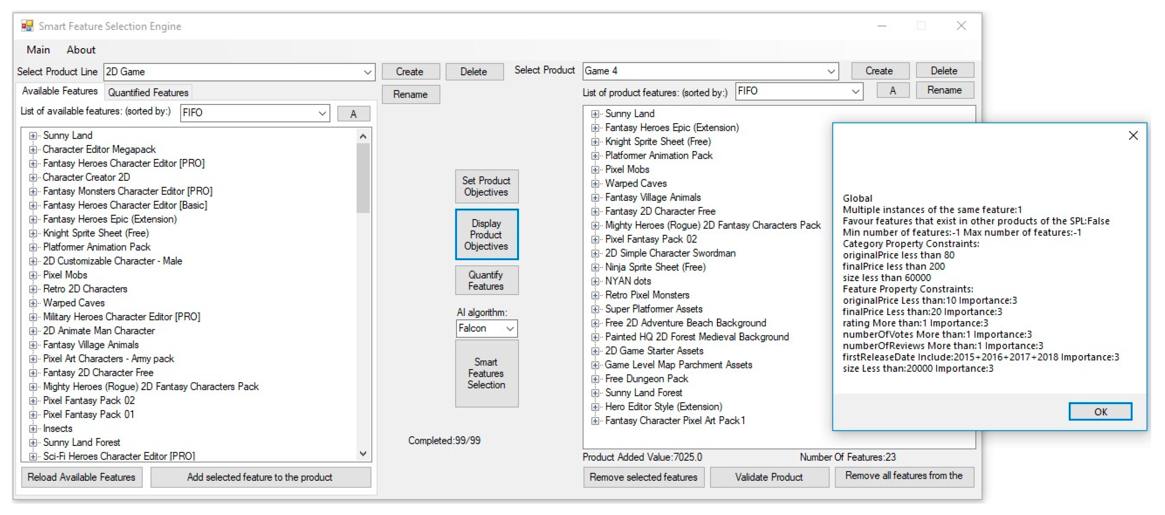
We evaluate the three Feature Selection Algorithms (FSAs), proposed in Section 4, in terms of product added value, execution time and number of selected features. The FSAs were applied on a dataset extracted from the Unity3D assets store [17], developed as part of this research. The experiments were executed in a custom-made tool called Feature Selection Engine (FSE) [16], also developed as part of this research. The experiment was conducted as follows; The original dataset was divided to 8 datasets [available in Supplementary file], containing 10, 20, 100, 1000, 6174, 10,000, 20,000, and 40,611 features. The raw datasets were imported to the FSE, where all features were quantified based on eight user-defined objectives. Three different user-defined product profiles, containing different product and category level objectives were set, in order to evaluate the algorithms. The FSE selected features based on the product profiles and the datasets containing the quantified features.

Evaluation of the dataset was performed using three case studies.

• Case Study-1: In this scenario, two product level constraints have been set: The total property value for the field “finalPrice” must be less than 500 and the total property value for the field “Size” must be less than 60,000.
• Case Study-2: In this scenario, one product level constraint has been set: The total property value for the field “finalPrice” must be less than 100.
• Case Study-3: In this scenario, three product level constraints have been set: The total property value for the field “finalPrice” must be less than 1000, the total property value for the field “numberOfVotes” must be greater than 5, and the total property value for the field “Size” must be less than 30,000. Along with these product level constraints, there is a constrain on the number of occurrences of a specific category, i.e., a category can appear only twice.

With all these three case studies, various parameters like time (in milliseconds), added value, and features added were obtained for the three feature selection algorithms on different datasets. Their outcome is averaged and provided in

Table 7. Average comparison between feature selection algorithms.

Algorithm (Features)	Time (Millisecond)	Added value	Features Added
Falcon (10)	5.33	1150.12	4.33
Jaguar (10)	4.67	1150.12	4.33
Snail (10)	336	1150.12	4.33
Falcon (20)	9	2061.03	7
Jaguar (20)	8.67	2057.64	7
Snail (20)	742,654.67	2061.03	7
Falcon (100)	37.33	6538.64	21
Jaguar (100)	35	5983.48	20.33
Falcon (1000)	1163	24511.07	66
Jaguar (1000)	430	30,331.39	86.67
Falcon (6174)	3080.67	55,372.52	184.33
Jaguar (6174)	5501	54,555.97	185.33
Falcon (10,000)	5845	84,594.1	291.33
Jaguar (10,000)	11,294.67	98,101.64	342.33
Falcon (20,000)	19,238.67	139,671.84	511.67
Jaguar (20,000)	47,739.67	155,199.57	560.67
Falcon (40,611)	85,979.33	384,726.32	1383.67
Jaguar (40,611)	226,166	448,012.86	1606.33

.

Table 7 is depicted in Figure 7, Figure 8 and Figure 9. In Table 7, the number of features provided in the first column indicates the eight datasets generated for evaluation purposes. In Figure 7, Figure 8 and Figure 9, it could be observed that the performance among the Falcon and Jaguar are close to each other due to presence of limited dataset. The Snail algorithm could be applied only for the first two datasets and thus not shown in the Figure 7, Figure 8 and Figure 9.

Observation from these figures reveal that Jaguar outperforms Falcon in terms of added value and features added. Meanwhile, Jaguar also consumes slightly higher time when considering the size of the dataset used. Thus, the importance of Jaguar in feature selection is justified, as Jaguar could result in 6% more of added value and 8% of number of features added, in average. In terms of execution time, Jaguar consumed 4% more than that of Falcon, on an average.

7. Conclusions and Future Work

This work presented novel way for quantifying dataset containing features based on multiple multi-level user-defined objectives. Quantification was performed for both numeric and text-based feature property values. Quantification considered the property values along with various operators. Furthermore, three feature selection algorithms considering user-defined objectives, named as Falcon, Jaguar, and Snail, were developed and evaluated. The three feature selection algorithms were evaluated using execution time, added value and number of features selected. Snail could obtain the best results in terms of added value but with a tradeoff in execution time. In average, Jaguar performed higher 6% and 8% in added value and number of features added, with an additional 4% increase in execution time. Additionally, during the execution of the algorithms, we captured the following metrics; number of features “attempted but not added” to the product, total property value “less than” and “more than” violations, minimum and maximum number of product/category features violation, and maximum number of features violation. These can be used as reference points for future improvements to the execution time of these algorithms and with other known algorithms. Enhancement to the quantification process can be done by providing a mechanism allowing the users to define conditions using a text-based language.