Article

Disentangled Feature Learning for Noise-Invariant Speech Enhancement

Department of Electrical and Computer Engineering and the Institute of New Media and Communications, Seoul National University, 1 Gwanak-ro, Gwanak-gu, Seoul 08826, Korea
*
Author to whom correspondence should be addressed.
Appl. Sci. 2019, 9(11), 2289; https://doi.org/10.3390/app9112289
Submission received: 29 April 2019 / Revised: 24 May 2019 / Accepted: 30 May 2019 / Published: 3 June 2019
(This article belongs to the Special Issue Advances in Deep Learning)

Abstract

:
Most of the recently proposed deep learning-based speech enhancement techniques have focused on designing the neural network architectures as a black box. However, it is often beneficial to understand what kinds of hidden representations the model has learned. Since the real-world speech data are drawn from a generative process involving multiple entangled factors, disentangling the speech factor can encourage the trained model to result in better performance for speech enhancement. With the recent success in learning disentangled representation using neural networks, we explore a framework for disentangling speech and noise, which has not been exploited in the conventional speech enhancement algorithms. In this work, we propose a novel noise-invariant speech enhancement method which manipulates the latent features to distinguish between the speech and noise features in the intermediate layers using adversarial training scheme. To compare the performance of the proposed method with other conventional algorithms, we conducted experiments in both the matched and mismatched noise conditions using TIMIT and TSPspeech datasets. Experimental results show that our model successfully disentangles the speech and noise latent features. Consequently, the proposed model not only achieves better enhancement performance but also offers more robust noise-invariant property than the conventional speech enhancement techniques.

Graphical Abstract

1. Introduction

Speech enhancement techniques aim to improve the quality and intelligibility of a given speech degraded by certain additive noise in the background. In a variety of applications, speech enhancement is considered as an essential pre-processing step. This technique can be directly employed to improve the quality of mobile communications [1] in noisy environments or to enhance speech signals for hearing aid devices [2,3] before amplification. Speech enhancement has also been widely used as a pre-processing technique in automatic speech recognition (ASR) [4,5] and speaker recognition systems [6] for more robust performances.
Over the past several decades, myriads of approaches have been developed in the speech research community for better speech enhancement. Spectral subtraction method [7] suppresses stationary noise from the input noisy speech by subtracting the spectral noise bias computed during the non-speech activity periods. The minimum mean-square error (MMSE)-based spectral amplitude estimator [8,9] showed promising results in terms of reducing residual noise as compared to the spectral subtraction method or Wiener filtering-based algorithm [10]. The least mean square adaptive filtering (LMSAF) based speech enhancement approaches have the best filtering performances of Wiener filter. Meanwhile, they do not need a priori knowledge, and can be adapted to the external environment by self-learning. But these approaches have some disadvantages including low constringency, strong sensitivity to non-stationary noise and a contradiction between constringency and stability [11,12]. The minima controlled recursive averaging (MCRA) noise estimation was also introduced in [13] of which the performance is known to be reasonably competitive under the environments with relatively high signal-to-noise ratios (SNR). However, since these statistical models are constructed based on a stationarity assumption, their performances generally tend to deteriorate in low SNR or highly non-stationary noise conditions. Non-negative matrix factorization (NMF) is one of the most common template-based approaches to speech enhancement [14,15,16], which models noisy observations as a weighted sum of non-negative source bases. NMF-based speech enhancement methods are more robust to non-stationary noise conditions as compared to the statistical model-based methods. These approaches, however, often result in signal distortion in the enhanced speech since they are based on an unrealistic assumption that speech spectrograms are linear combinations of the basis spectra.
Due to the complex nature of the noise corruption process, non-linear models such as deep neural networks (DNNs) have been suggested as an alternative choice for modeling the relationship between the noisy and the corresponding clean speech utterances. DNNs have been successful in solving the speech enhancement tasks under various noise environments since its introduction. Early literature using DNNs as a nonlinear mapping function for estimating clean speech had reported better enhancement results [17,18,19,20] compared to the NMF-based algorithms. Various neural network structures have been employed for speech enhancement, such as multi-context stacking networks for ensemble learning [21], recurrent neural networks (RNNs) [22,23,24], and convolutional neural networks (CNNs) [25,26].
More recently, generative adversarial network (GAN) [27] has become popular in the area of deep learning, and it has been also applied to speech enhancement. Pascual et al. proposed end-to-end speech enhancement GAN (SEGAN) in which the generator learns to model the mapping from the noisy speech samples to their clean counterparts, while the discriminator learns to distinguish between the enhanced and the target clean samples within the context of a mini-max game [28]. The underlying idea of GAN has been adopted in many GAN-based speech enhancement algorithms including the time-frequency mask estimation using the minimum mean square error GAN (MMSE-GAN) [29] and the conditional GAN (cGAN) [30].
Though deep learning-based speech enhancement models have achieved considerable improvements, the performance is usually degraded in the case of mismatched conditions caused by different types of noises or SNR levels between the training and test set samples. Moreover, the performance varies depending on the types of noises. In order to address such issues, disentangled feature learning can be considered as a possible solution. Most of the previous studies [17,18,19,20,21,22,23,24,25,26,27,28,29,30], which have focused mainly on the mapping between the noisy and the clean speech, rarely consider how input features are learned in the hidden layers. The model based on disentangled feature learning, on the other hand, manipulates the latent features to distinguish between the speech and noise in the intermediate layers, hence resulting in better enhancement performance even in the mismatched noise conditions. Moreover, the quality of noise-invariant attributes can also be improved.
In this paper, we propose a novel deep learning-based noise-invariant speech enhancement algorithm which employs an adversarial training framework designed to disentangle the latent features of speech and noise, under the concept of domain adversarial training (DAT) [31]. Although DAT was originally introduced for the domain adaptation task, the proposed algorithm exploits the DAT framework for use in the regression task, i.e., speech enhancement. Experimental results show that the proposed method successfully disentangles the speech and noise latent features. Moreover, the results also reveal that our model outperforms the conventional DNN-based algorithms. The main contributions of this paper are summarized as follows:
  • We modify the DAT framework in order to solve the speech enhancement task in a supervised manner. The proposed model achieves better performance in speech enhancement as compared to the baseline models under both the matched and mismatched noise conditions.
  • By reducing the performance gap among different noise types, we show that our method is more robust to noise variability.
  • By visualizing feature representations, we demonstrate that our model successfully disentangles speech and noise latent features.
The remainder of this paper is organized as follows: Section 2 reviews past studies related to the proposed method. The proposed model is elaborately described in Section 3. Section 4 reports the results obtained from the experiments and discusses the details. Finally, Section 5 concludes the paper.

2. Related Work

2.1. Masking-Based Speech Enhancement

When training neural networks in a supervised manner, it is essential to define a proper training target in order to ensure effective learning. The training targets for speech enhancement can be mainly categorized into two groups: (i) mapping-based, and (ii) masking-based approaches. The mapping-based methods learn a regression function relating a noisy speech to the corresponding clean speech directly while the masking-based methods estimate time-frequency masks given a noisy speech. A variety of training targets have been studied. Wang et al. evaluated and compared the performance of various mapping-based and masking-based targets [32]. It may be controversial to argue which method is better, yet many cases have shown that the masking-based methods (e.g., ideal ratio masks) tend to perform better than the mapping-based methods [21,32,33] in terms of enhancement results. In this work, we design the proposed model within a masking-based framework. We use the time-frequency masking functions as an extra layer in the neural network [22]. This way, the model implicitly incorporates the masking functions when optimizing the network which will be detailed in Section 3.1.

2.2. Domain Adversarial Training

Domain adaption [34] addresses the problem of mismatch between the training and test datasets by transferring the knowledge learned from the source domain to a robust model in the target domain. DAT is one of the approaches that attempts to match the data distributions across different domains. In [31], DAT exploits an adversarial training method in order to learn intermediate features which are invariant to the shifts in data from different domains. Here, the neural network learns two different classifiers: (i) a classifier for the main classification task, and (ii) the domain classifier. The training objective of the domain classifier, in particular, is to learn whether the input sample is from the source or target domain, given features extracted using labeled data from the source domain and unlabeled data from the target domain. The feature extractor is shared by both the main task and the domain classifiers. In implementation, a gradient reversal layer (GRL) is employed to act as an identity transformer in the forward-propagation and to reverse the gradient by multiplying a negative scalar during the back-propagation [31]. Consequently, the GRL encourages the latent features to act discriminatively when solving the main classification task, yet act indiscriminately towards the shifts across different domains. In other words, the feature extractor is trained so that the model maps data from different domains to the latent features with similar distributions via adversarial learning.
Many speech processing frameworks have adopted the idea of DAT in order to extract domain-invariant features. Under the noise robust speech recognition scheme, the clean speech was regarded as the source domain data and was used to train the senone label classifier, while the noisy speech played the role of the target domain data to be adjusted by the feature extractor [35,36]. DAT was also used to learn speaker-invariant senone labels, as shown in [37] where the adversarial training successfully aligned the feature representation of different speakers. In [38], the authors demonstrated that accent-invariant features could be learned for the ASR system. For speaker recognition tasks, DAT was adopted to tackle the channel mismatch problem. In particular, the latent features were extracted in order to learn channel-invariant, yet speaker-discriminative representations [39]. In [40], the authors showed that DAT was able to adapt multiple forms of mismatches (e.g., speaker, acoustic conditions, and emotional content) when solving the acoustic emotion recognition task. As for the speech enhancement problems, a noise adaptive method exploiting DAT was proposed in [41]. In their work, however, DAT was only used to classify stationary and non-stationary noises, and the authors did not make use of various noise components for domain-invariant regression.

3. Proposed Method

In this section, we propose a method to disentangle the speech and noise features for noise-invariant speech enhancement. We present (1) the proposed model architecture, (2) objective functions, and (3) the adversarial learning process.

3.1. Neural Network Architecture

Our neural network consists of five sub-networks: (i) an encoder (E), (ii) a speech decoder ( D s ), (iii) a noise decoder ( D n ), (iv) a noise disentangler ( D E n ), and (v) a speech disentangler ( D E s ). The overall architecture of the proposed model is illustrated in Figure 1.
We extracted the magnitude spectra as the raw features of all signal components. Only the magnitude spectra were estimated while the phase parts of the noisy speech are kept intact. Let us denote the magnitude spectra of the noisy speech, clean speech, and noise as x R F × ( 2 τ + 1 ) , s R F × 1 , and n R F × 1 , respectively, where F denotes the number of frequency bins and τ represents an input context expansion parameter (i.e., one current frame, τ previous and τ next frames). The encoder E learned a function that maps x into speech and noise latent features, defined by the neural network parameter θ E as follows:
( z s , z n ) = E ( x ; θ E ) ,
where z s R M × 1 and z n R M × 1 indicate M-dimensional speech and noise latent features, respectively. Similarly, D s and D n learn mappings parameterized by θ D s and θ D n , respectively, as follows:
m ^ s = D s ( z s ; θ D s ) , m ^ n = D n ( z n ; θ D n ) ,
where m ^ s R F × 1 and m ^ n R F × 1 denote the estimated speech and noise masks, respectively. The time-frequency masks were constrained such that the sum of the estimated values should be equal to the input noisy speech. Given the masks from both of the decoders, we can obtain the predicted speech and noise through a deterministic layer [22]. Given m ^ s and m ^ n , the predicted magnitude spectra of speech s ^ R F × 1 and noise n ^ R F × 1 can be calculated as
s ^ = m ^ s m ^ s + m ^ n x , n ^ = m ^ n m ^ s + m ^ n x ,
where the addition, division, and product (⊗) operators were executed element-wise.
Finally, D E n and D E s were trained to separate the noise attributes from the speech latent features, and vice versa. D E n and D E s are respectively parameterized by θ D E n and θ D E s as follows:
n ˜ = D E n ( z s ; θ D E n ) , s ˜ = D E s ( z n ; θ D E s ) ,
where s ˜ R F × 1 and n ˜ R F × 1 represent the speech and noise components, respectively estimated from the latent features. Note that s ˜ and n ˜ differ from s ^ and n ^ in Equation (3). s ˜ and n ˜ were generated by the disentanglers which were trained to make the encoder difficult to predict the speech and noise. The GRLs are inserted between the encoder and the disentanglers to establish an adversarial setting. On the other hand, s ^ and n ^ were well estimated by the corresponding decoders.
In the final speech enhancement stage, after obtaining s ^ from the decoders, the estimated clean speech spectrum S ^ was reconstructed by
S ^ = s ^ exp ( j x ) ,
where x denotes the phase of the corresponding input noisy speech. S ^ is then transformed to the time-domain signal through inverse discrete Fourier transform (IDFT). Finally, an overlap-add method as in [42] is used to synthesize the waveform of the enhanced speech.

3.2. Training Objectives

Given the estimates s ^ and n ^ of the clean speech s and noise n , we optimized the neural network parameters of the encoder and decoders by minimizing the mean squared error defined as follows:
L D s ( θ E , θ D s ) = 1 K k = 1 K s k s ^ k 2 , L D n ( θ E , θ D n ) = 1 K k = 1 K n k n ^ k 2 ,
where · indicates the l 2 -norm, K is the number of mini-batch size, and s ^ k ( n ^ k ) is the estimate of the k-th speech (noise) sample s k ( n k ) in the mini-batch. Similarly, we also train the encoder and the disentanglers by using the following objective functions:
L D E n ( θ E , θ D E n ) = 1 K k = 1 K n k n ˜ k 2 , L D E s ( θ E , θ D E s ) = 1 K k = 1 K s k s ˜ k 2 ,
where n ˜ k and s ˜ k are obtained through Equation (4). To obtain disentangled features, we minimize L D E n and L D E s defined in Equation (7) with respect to θ D E n and θ D E s , while maximizing them with respect to θ E simultaneously. Combining Equations (6) and (7), the total loss of the proposed network was formulated as
L T ( θ E , θ D s , θ D n , θ D E n , θ D E s ) = [ L D s ( θ E , θ D s ) λ 1 L D E n ( θ E , θ D E n ) ] + α [ L D n ( θ E , θ D n ) λ 2 L D E s ( θ E , θ D E s ) ] ,
where λ 1 and λ 2 are positive hyper-parameters which control the amount of gradient reversal in the back-propagation step, and α denotes the weight controlling the contribution of the noise estimate.
In recent studies [35,36,37,38,39,40,41], GRL has only been used for domain predictions under narrowly restricted settings (with only two possible domains, e.g., the source and the target) or for classifications of channels, speakers, and noise types. The proposed model distinguishes itself from the past approaches by using two GRLs to disentangle the speech and noise latent features in a regression manner.

3.3. Adversarial Training for Disentangled Features

Neural network parameters are optimized by using the objective function given in Equation (8) via adversarial learning. D s and D n are trained to minimize L D s and L D n , and D E n and D E s are also trained to minimize L D E n and L D E s . As for the optimization of E, it was essential to ensure that it should produce disentangled features. This idea was implemented by minimizing L D s and L D n while maximizing L D E n and L D E s in an adversarial manner with respect to the encoder parameter θ E . Such a mini–max competition eventually converges to the point where the encoder network generates the noise-confusing latent feature z s and the speech-confusing latent feature z n , disentangled in the latent feature space. D s and D n then use z s and z n as input respectively and produce noise-invariant speech s ^ . In summary, optimizations of the network parameters are given by
( θ ^ E , θ ^ D s , θ ^ D n ) = arg min θ E , θ D s , θ D n L T ( θ E , θ D s , θ D n , θ ^ D E n , θ ^ D E s ) , ( θ ^ D E n , θ ^ D E s ) = arg max θ D E n , θ D E s L T ( θ ^ E , θ ^ D s , θ ^ D n , θ D E n , θ D E s ) ,
where θ ^ ( · ) denotes the optimal parameters for each given network ( · ) .
The network parameters defined by Equation (9) can be found as a stationary point of the following gradient updates:
θ E θ E μ ( L D s θ E + α L D n θ E λ 1 L D E n θ E α λ 2 L D E s θ E ) , θ D s θ D s μ L D s θ D s , θ D n θ D n μ α L D n θ D n , θ D E n θ D E n μ L D E n θ D E n , θ D E s θ D E s μ α L D E s θ D E s ,
where μ indicates the learning rate. The updates of Equation (10) are very similar to stochastic gradient descent (SGD) updates for the feed-forward deep model that comprises the encoder fed into the decoders and into the disentanglers. The difference was that the gradients from the decoders and disentanglers were subtracted with loss weighted by λ 1 , λ 2 , and α , instead of being summed. The negative coefficient λ 1 and λ 2 enable the encoder to induce the maximization of L D E n and L D E s by reversing the gradients during the back-propagation. If both λ 1 and λ 2 were set to zero, the neural network structure presented in Figure 1 became equivalent to the conventional DNN structure. The optimized networks E, D s and D n were then used during the test stage for generating the clean speech estimates given the noisy test speech samples.

4. Experiments and Results

In this section, we evaluate the performance of the proposed model compared to the baseline systems using various metrics. For performance comparison, we conducted experiments in both the matched and mismatched noise conditions.

4.1. Dataset

We used 6300 utterances of clean speech data from the TIMIT database [43] to train the neural networks. TIMIT database consists of 10 sentences, each spoken by 630 English speakers. In order to make sure that various noisy utterances are considered during simulations, we selected 10 different noise types including: car, construction, office, railway, cafeteria, street, incar, train, bus from ITU-T recommendation P.501 database [44] and white noise from NOISEX-92 database [45]. In the case of matched noise conditions, two-thirds of each noise clip was used for training and the rest for testing. For each pair of the clean speech utterance and the noise waveform, a noisy speech utterance was artificially generated with an SNR value randomly chosen from 3 to 6 dB in 1 dB scale. As a result, a total of 63,000 utterances (about 54 h) were used so that the entire database was mixed with each noise type.
The test set consisted of 1400 utterances of clean speech data from TSPspeech [46], spoken by 12 male and 12 female English speakers. For the experiments in the matched noise conditions, we used the same noise types as used for training. For the experiments in the mismatched noise conditions, noises including kids, traffic, metro, and restaurant from ITU-T recommendation P.501 database were applied. Noisy speech utterances were generated with the SNR value ranging from 6 to 9 dB with 3 dB step in which 6 and 9 dB cases represented the unseen SNR conditions.

4.2. Feature Extraction

The input and target features of the networks were extracted in the following way. First, we extracted the magnitude spectra from the noisy speech, the corresponding clean speech, and noise. A 512-point Hamming window with 50 % overlap was applied to the audio signals, sampled at 16kHz, and then short-time Fourier transform (STFT) was applied. 512 points STFT magnitudes were reduced to 257 points by removing the symmetric half. F and τ were fixed to 257 and 5, respectively. Thus, input feature vectors, extracted from 11 consecutive frames, were concatenated in a similar manner as in [19].

4.3. Network Setup

The network architecture of the proposed model is presented in Figure 1, in which we refer to the speech-noise disentangled training ( s n D T ) model. The encoder E was constructed by stacking two hidden layers with 2048 leaky rectified linear units (ReLUs) [47] in each layer. The number of the input nodes of E was 257 × 11 = 2827 . The output layer generated two separated outcomes of 512 nodes (i.e., the dimension M of z s and z n ) with leaky ReLUs.
The decoders D s and D n also had two hidden layers with 2048 leaky ReLUs in each layer. The numbers of the input and output nodes in each network were 512 and 257, respectively. For the output activations, Sigmoid was used to restrict the output mask ( m ^ s and m ^ n ) values to be in [0, 1], yet s ^ and n ^ were determined implicitly by Equation (3). The structures of D E n and D E s were identical to that of D s except for the output activation functions. ReLUs were used for the output magnitudes ( s ˜ and n ˜ ).
The s n D T model was trained with Adam optimizer [48], with a learning rate of 1 × 10⁻³, using a mini-batch size of 10 utterances. Batch normalization [49] was applied to all of the hidden and output layers for regularization and stable training. As for the hyper-parameters λ 1 and λ 2 of Equation (8), we took an approach similar to [31]. λ 1 and λ 2 were initialized with 0 for the first 50 K training iterations, and then their values were gradually increased until reaching ( λ 1 , λ 2 ) = 0.3 by the end of the training. α in Equation (8) was fixed at 0.4. Figure 2 shows the training losses obtained from the s n D T model, and it is seen that the model was trained properly. Through the adversarial training as defined by Equation (9), the speech and noise estimation losses decreased, and the disentangling losses increased gradually to convergence.
To evaluate the performance of the disentangled feature learning technique, we implemented three baseline models for comparison. These baseline systems are as follows:
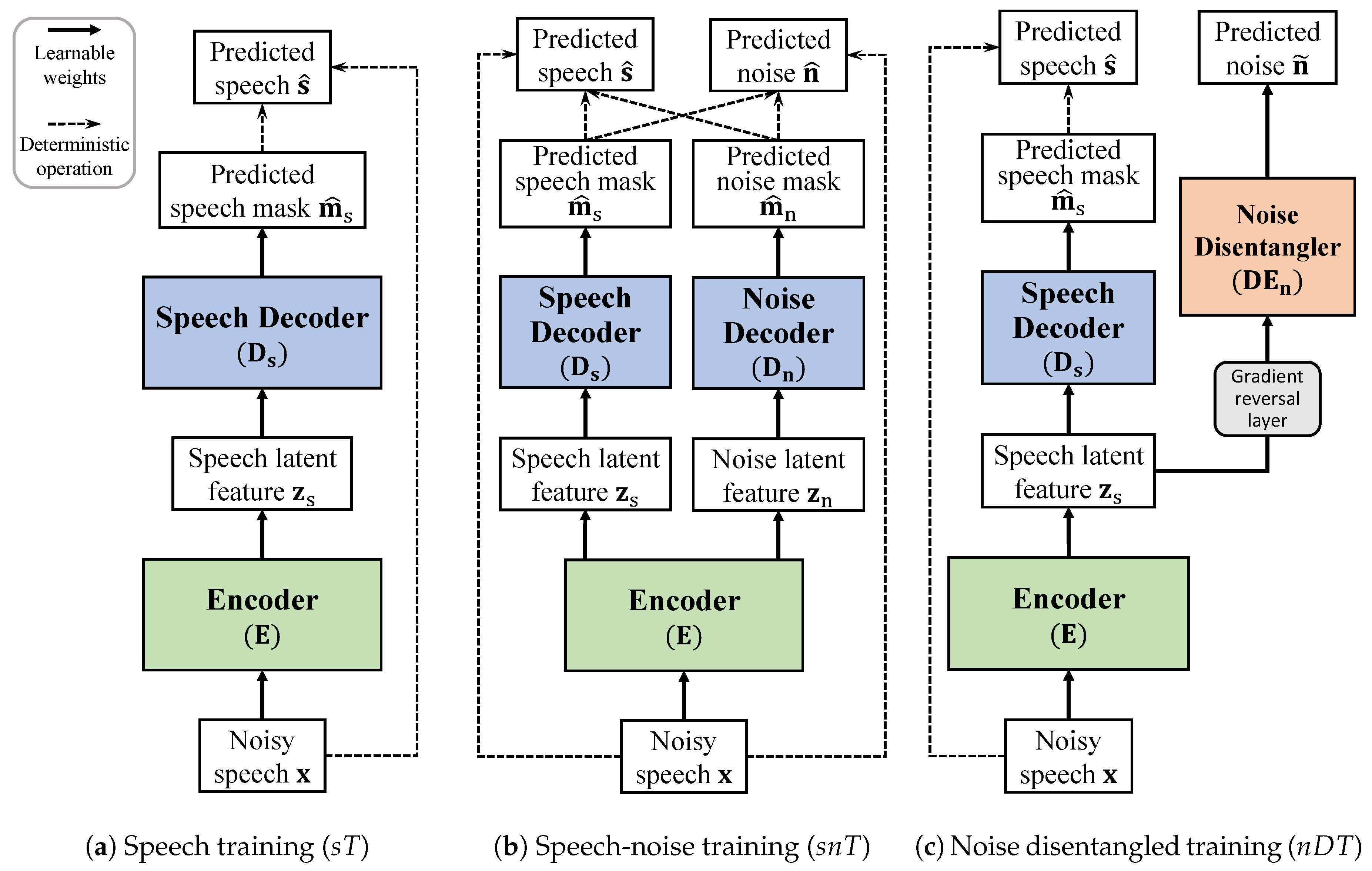
  • Speech training ( s T ) model, as shown in Figure 3a, was a deep denoising autoencoder [17], and it took a regression approach closely resembling [19].
  • Speech-noise training ( s n T ) model, as shown in Figure 3b, utilized noise components to construct the time-frequency masks. This approach was similar to the method suggested in [22]. Unlike the s n D T model, however, the s n T model did not exploit disentangled feature learning.
  • Noise disentangled training ( n D T ) model, as shown in Figure 3c, was trained so that the noise components were disentangled from the speech latent features without using noise latent features.
The baseline models were configured similarly in terms of hyper-parameters, the number of layers and nodes in each module, to ensure a fair comparison with the s n D T model. We implemented all the networks using Tensorflow [50].

4.4. Objective Measures

For the evaluation of the models’ performances, we considered four different aspects, speech quality, noise reduction, speech intelligibility, and speech distortion. The tested objective measures are summarized as in the following:
  • PESQ: Perceptual evaluation of speech quality defined in the ITU-T P.862 standard [51].
  • segSNR: Segmental SNR, which is the average of the SNR per frame for the two speech signals [52]
  • eSTOI: Extended short-time objective intelligibility [53].
  • SDR: Signal-to-distortion ratio [54].
All metric values for the enhanced speech were compared with the corresponding clean reference of the test set.

4.5. Performance Evaluation

In case of the matched noise conditions, we measured the objective metrics and averaged them over each SNR environment to evaluate performance for ten different noise types. Table 1 presents the PESQ scores, segSNR, eSTOI, and SDR values obtained in the matched noise conditions where the column “ n o i s y ” refers to the results obtained from the clean and the unprocessed noisy speech. The cases with SNR equal to 6 and 9 dB indicate the unseen SNR conditions that were not included during the training phase. Firstly, we investigated whether the use of noise information improves performance for speech enhancement. The results show that the s n T model, which constructed the masks using both speech and noise information, performed better than the s T model whose prediction was based only on speech components. Similarly, the s n D T model with noise estimates reported better performance in terms of all the metrics compared to the n D T model.
The n D T model, which disentangles the noise components in the latent feature space, resulted in lower performance improvements in comparison with the s n T model. This confirms that even though the n D T model incorporated disentangled feature learning, it was not able to exploit the noise information to construct the masks during the speech enhancement process. On the other hand, in order to examine the sole effect of the disentangled feature learning, the n D T model should be compared to the s T model whose structure is identical to the n D T model except for the noise disentangler. As can be seen in the results, the n D T model outperformed the s T model in terms of all the metrics. Furthermore, the comparison of the s n D T model to the s n T model, both of which similarly adopted the masks except that the s n D T model additionally applied disentangled feature learning, reported better performance improvements for the s n D T model. In summary, the proposed model showed better performance than all the other baseline models in terms of speech quality, intelligibility, noise reduction, and speech distortion, indicating that the disentanglement between speech and noise features in the latent feature space was more effective for the prediction of the clean speech.
In case of the mismatched noise conditions, we evaluated performance given four different noise types and averaged the results over each of the SNR environment. Table 2 presents the PESQ scores, segSNR, eSTOI, and SDR values obtained under the mismatched noise conditions. The results show that the s n D T model outperformed the baseline methods, implying that it was more robust to the unseen noise types. Since the s n D T model learned how to disentangle speech components from the latent features, the disentangled features could be obtained even in the mismatched noise conditions. From the perspective of noise reduction, in particular, it is quite noteworthy that the models using disentangled feature learning showed relatively competitive performance improvements in the mismatched noise conditions compared to the matched conditions. In case of the matched noise conditions, the relative improvement of segSNR was 16.31 % for the n D T model when compared against the s T model, and 11.21 % for the s n D T model against the s n T model. In the case of the mismatched noise conditions, however, the relative improvements of segSNR of the n D T and s n D T models were 38.79 % and 15.95 % , respectively. It can be seen that the proposed approach is particularly effective in the aspect of noise reduction.
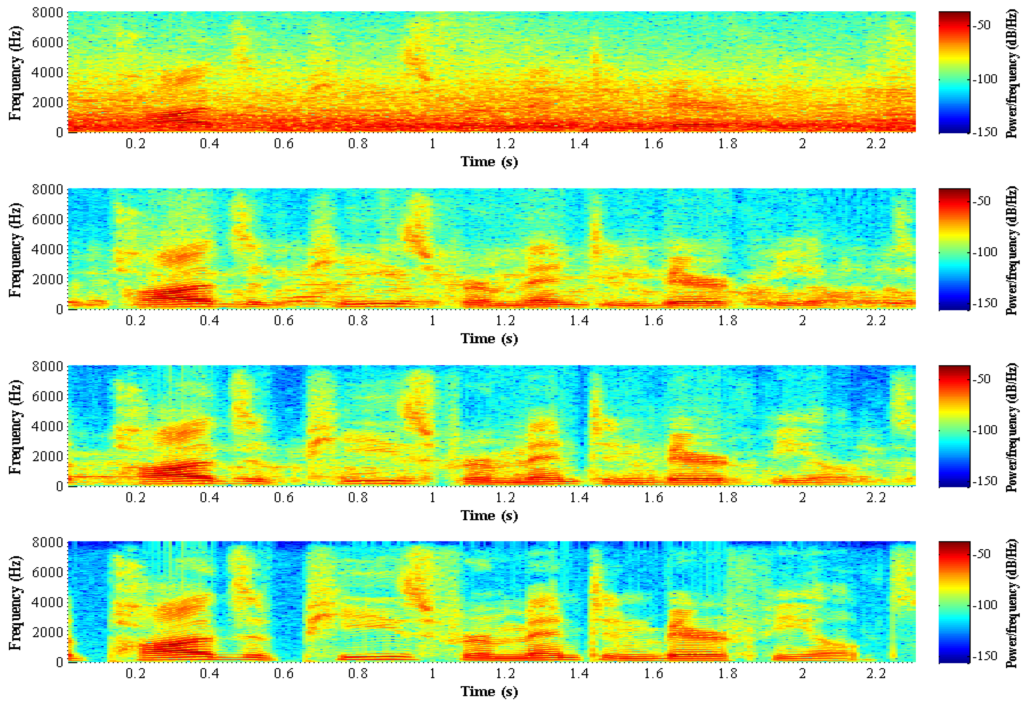
Additionally, Figure 4 shows the spectrograms of an utterance enhanced by the s n T and s n D T models in the mismatched noise conditions. From this figure, it is shown that the proposed algorithm effectively reduced the noise from the original noisy speech while the speech distortion was minimized.

4.6. Subjective Test Results

We also conducted a listening test to compare the subjective performance of the proposed algorithm with the conventional scheme. For that, 18 listeners participated and were presented with 42 randomly selected sentences corrupted by the 14 different noises in the SNR values of −3, 0, and 3 dB. In the test, each listener was provided with speech samples enhanced by the s n T model and s n D T model. Listeners could listen to each enhanced speech as many times as they wanted, and were asked to choose the preferred one from each pair of speech samples in terms of perceptual speech quality. If the quality of the two samples was indistinguishable, listeners could select no preference. Two samples in each pair were given in arbitrary order.
The results are shown in Figure 5. It can be seen that the quality of the speech enhanced by the proposed model was better than the conventional model in all SNR values. With respect to the averaged results, the s n D T model was preferred to the s n T model in 52.78 % of the cases, while the opposite preference was 8.20 % (no preference in 39.02 % of the cases). These results imply that the proposed algorithm enhances not only the objective measures but also the perceived quality.

4.7. Analysis of Noise-Invariant Speech Enhancement

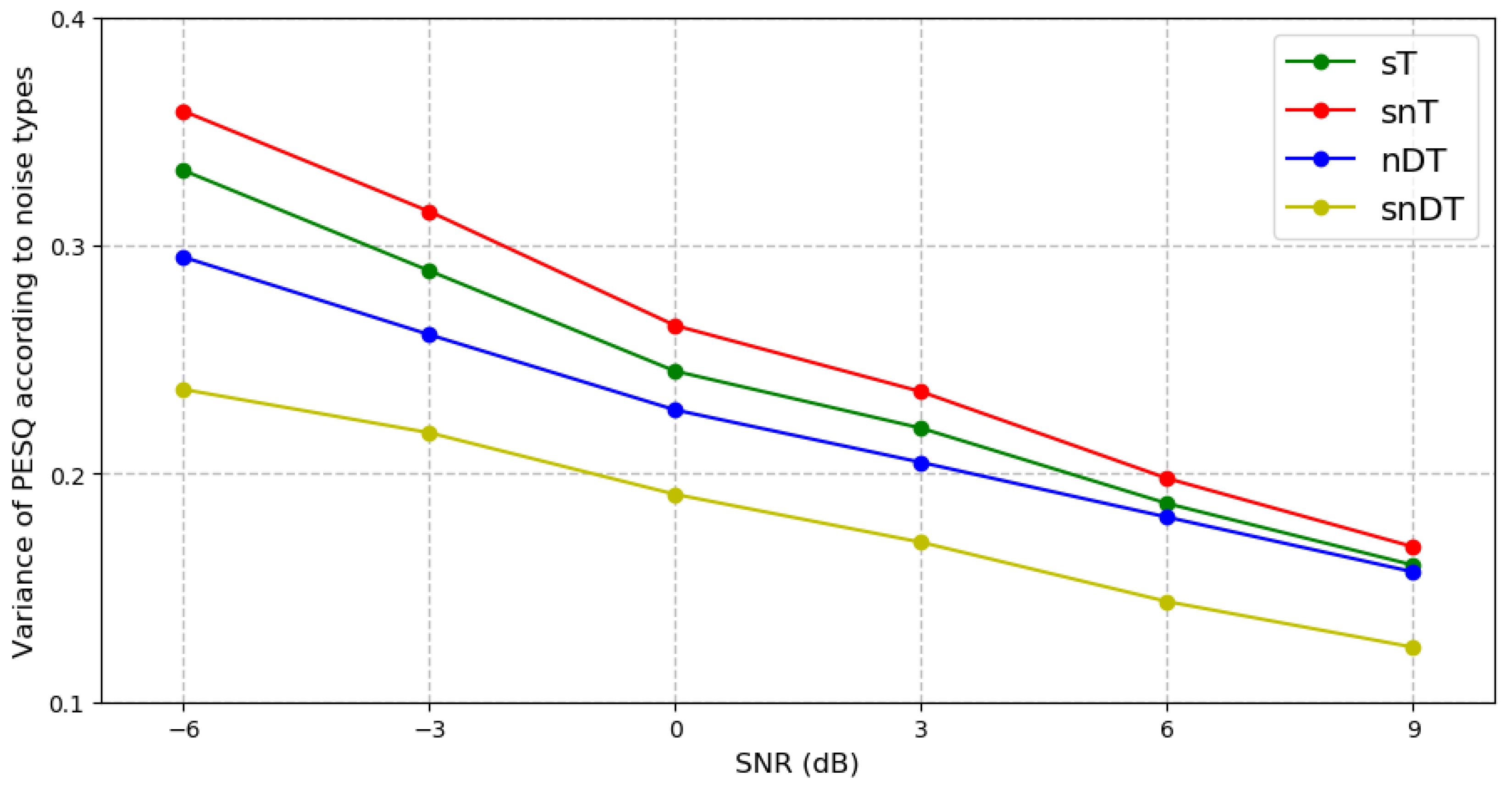
As the network is trained with different types of noise, it is easily anticipated that the performance may vary depending on the noise types even when given the same SNR value. This could be problematic, especially under various real-world noise environments, because lower performance improvements for certain noise types could certainly result in lower performance in overall for the entire system. Figure 6 describes the variances of the PESQ scores obtained from different noise types. We separately measured the PESQ scores for each noise type and computed the variances of 14 different noise types used in the matched and mismatched noise conditions. The results show that the proposed algorithm yielded the smallest performance gap among the noise types in all of the SNR environments. It is noted that the s n D T model produced much smaller variances at the low SNR level compared to the baseline models. This demonstrates that the proposed model was less sensitive to different noise types during the enhancement process because it disentangled the speech attributes well from the noisy speech in the latent feature space. Experimental results, therefore, suggest that the proposed model is a speech enhancement system with an improved noise-invariant property.

4.8. Disentangled Feature Representations

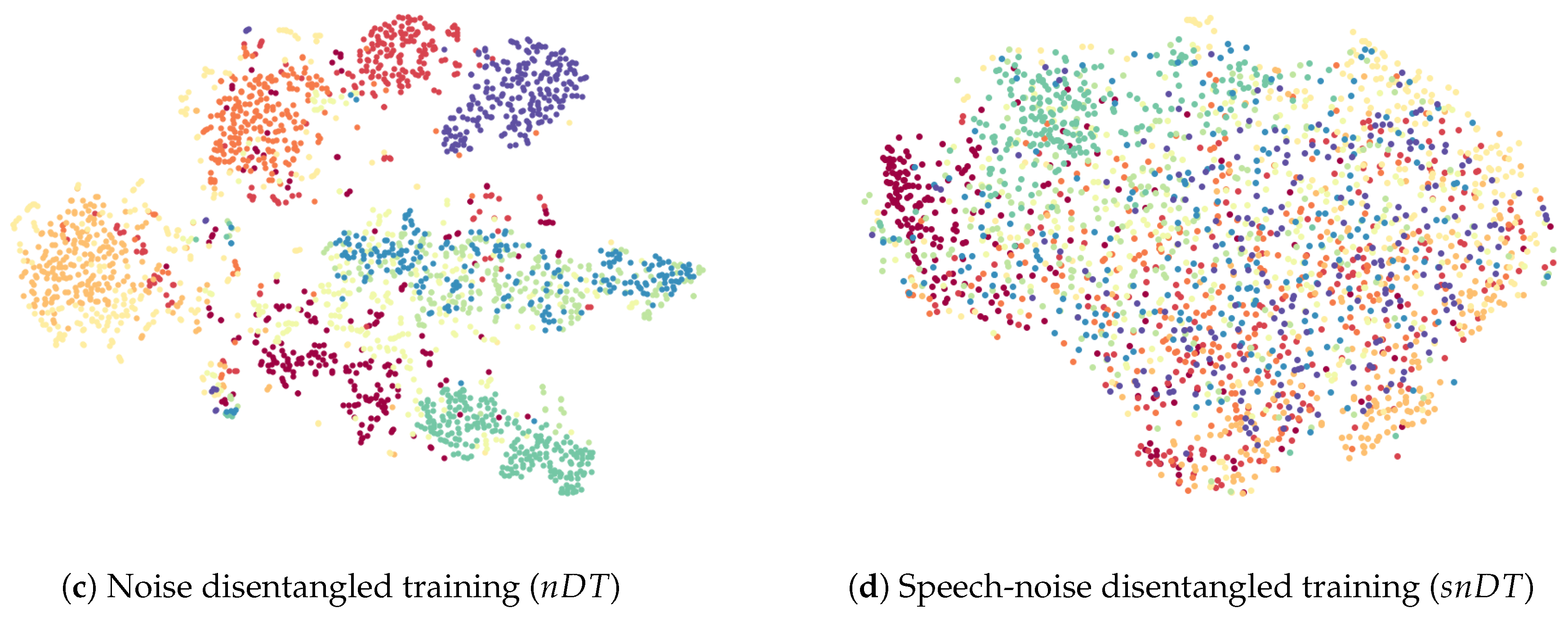
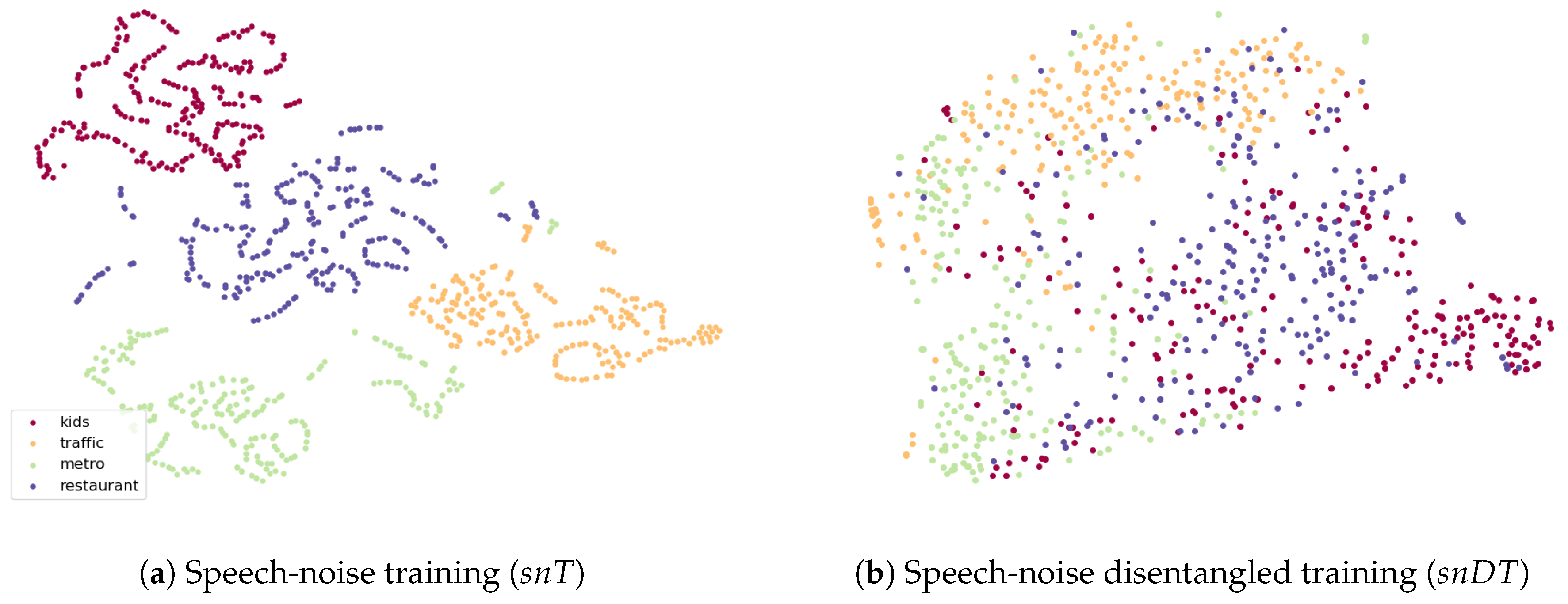
We further explored the effect of disentangled feature learning by visualizing the speech latent feature ( z s ) using t-distributed stochastic neighbor embedding (t-SNE) [55]. The t-SNE is a popular data visualization method which projects high dimensional data into a subspace with a smaller dimension. The projection serves as a useful tool to visually inspect feature representations learned by the model. We extracted speech latent features from a subset of the test samples through trained models and projected the 512-dimensional z s into the two-dimensional space using t-SNE. Figure 7 visualizes the speech latent feature representations obtained in the matched noise conditions. Figure 7d, in particular, shows that by using two disentanglers for adversarial learning, the distribution of z s became almost indistinguishable. This implies that the noise attributes were highly likely to be disentangled in z s . In contrast, without disentangled feature learning, as shown in Figure 7a,b, we were able to separate each type of noise cluster easily in the latent feature space. This indicates that the noise attributes remain intact in z s . Figure 7c shows that the n D T model disentangled the noise components more clearly as compared to the s T and s n T models, yet not as much as the s n D T model. Finally, Figure 8 shows the speech latent feature representations in the mismatched noise conditions. Even though the noise types were not included in the training data, the proposed model disentangled noise components more clearly in the latent feature space compared to the conventional DNN-based models.

5. Conclusions

In this paper, we proposed a novel speech enhancement method in which speech and noise latent features were disentangled via adversarial learning. In order to explore the disentangled representation which has not been exploited in the conventional speech enhancement algorithms, we designed a model using GRLs. The proposed architecture is composed of five sub-networks where the decoders and the disentanglers were trained in an adversarial manner to encourage the encoder to produce noise-invariant features. The speech latent features generated by the encoder reduced the variability among different noise types while retaining the speech information intact. Experimental results showed that the proposed model outperformed the conventional DNN-based speech enhancement algorithms in terms of various measurements in both the matched and mismatched noise conditions. Moreover, the proposed model achieved more competitive noise-invariant property through disentangled feature learning. Visualization of the speech latent features demonstrated that the proposed method was able to disentangle speech attributes from the noisy speech in the latent feature space.
In our future work, we will further develop novel structures and training techniques for a better representation of disentangled speech and noise features than the current model. In addition, we will consider a model that can disentangle the various factors that occur in voice communication systems.

Author Contributions

Conceptualization, S.H.B. and N.S.K.; methodology, S.H.B.; software, S.H.B.; validation, S.H.B. and N.S.K.; formal analysis, S.H.B.; investigation, S.H.B.; data curation, S.H.B. and I.C.; writing—original draft preparation, S.H.B.; writing—review and editing, N.S.K.; visualization, S.H.B. and I.C.; supervision, N.S.K.; project administration, S.H.B. and N.S.K.; funding acquisition, N.S.K.

Funding

This work was supported by the research fund of Signal Intelligence Research Center supervised by Defense Acquisition Program Administration and Agency for Defense Development of Korea.

Conflicts of Interest

The authors declare no conflict of interest.

References

  1. Kim, N.S.; Chang, J.H. Statistical model based techniques for robust speech communication. In Recent Advances in Robust Speech Recognition Technology; Bentham Science: Sharjah, UAE, 2010; pp. 114–132. [Google Scholar]
  2. Chen, J.; Wang, Y.; Yoho, S.E.; Wang, D.; Healy, E.W. Large-scale training to increase speech intelligibility for hearing-impaired listeners in novel noises. J. Acoust. Soc. Am. 2016, 139, 2604–2612. [Google Scholar] [CrossRef] [PubMed] [Green Version]
  3. Lai, Y.H.; Chen, F.; Wang, S.S.; Lu, X.; Tsao, Y.; Lee, C.H. A deep denoising autoencoder approach to improving the intelligibility of vocoded speech in cochlear implant simulation. IEEE Trans. Biomed. Eng. 2017, 64, 1568–1578. [Google Scholar] [CrossRef] [PubMed]
  4. Maas, A.L.; Le, Q.V.; O’neil, T.M.; Vinyals, O.; Nguyen, P.; Ng, A.Y. Recurrent neural networks for noise reduction in robust ASR. In Proceedings of the INTERSPEECH, Portland, OR, USA, 9–13 September 2012; pp. 22–25. [Google Scholar]
  5. Donahue, C.; Li, B.; Prabhavalkar, R. Exploring speech enhancement with generative adversarial networks for robust speech recognition. In Proceedings of the IEEE International Conference on Acoustics, Speech and Signal Processing (ICASSP), Calgary, AB, Canada, 15–20 April 2018; pp. 5024–5028. [Google Scholar]
  6. Ortega-García, J.; González-Rodríguez, J. Overview of speech enhancement techniques for automatic speaker recognition. In Proceedings of the Fourth International Conference on Spoken Language Processing, Philadelphia, PA, USA, 3–6 October 1996; pp. 929–932. [Google Scholar]
  7. Boll, S.F. Suppression of acoustic noise in speech using spectral subtraction. IEEE Trans. Acoust. Speech Signal Process. 1979, 27, 113–120. [Google Scholar] [CrossRef]
  8. Ephraim, Y.; Malah, D. Speech enhancement using a minimum-mean square error short-time spectral amplitude estimator. IEEE Trans. Acoust. Speech Signal Process. 1984, 32, 1109–1121. [Google Scholar] [CrossRef] [Green Version]
  9. Kim, N.S.; Chang, J.H. Spectral enhancement based on global soft decision. IEEE Signal Process. Lett. 2000, 7, 108–110. [Google Scholar]
  10. Lim, J.S.; Oppenheim, A.V. All-pole modeling of degraded speech. IEEE Trans. Acoust. Speech Signal Process. 1978, 26, 197–210. [Google Scholar] [CrossRef]
  11. Gupta, P.; Patidar, M.; Nema, P. Performance analysis of speech enhancement using LMS, NLMS and UNANR algorithms. In Proceedings of the IEEE International Conference on Computer, Communication and Control (IC4), Madhya Pradesh, India, 10–12 September 2015; pp. 1–5. [Google Scholar]
  12. Li, R.; Liu, Y.; Shi, Y.; Dong, L.; Cui, W. ILMSAF based speech enhancement with DNN and noise classification. Speech Commun. 2016, 85, 53–70. [Google Scholar] [CrossRef]
  13. Cohen, I.; Berdugo, B. Speech enhancement for non-stationary noise environments. Signal Process. 2001, 81, 2403–2418. [Google Scholar] [CrossRef]
  14. Kwon, K.; Shin, J.W.; Kim, N.S. NMF-based speech enhancement using bases update. IEEE Signal Process. Lett. 2015, 22, 450–454. [Google Scholar] [CrossRef]
  15. Wilson, K.W.; Raj, B.; Smaragdis, P.; Divakaran, A. Speech denoising using nonnegative matrix factorization with priors. In Proceedings of the IEEE International Conference on Acoustics, Speech and Signal Processing (ICASSP), Las Vegas, NV, USA, 30 March–4 April 2008; pp. 4029–4032. [Google Scholar]
  16. Mohammadiha, N.; Smaragdis, P.; Leijon, A. Supervised and unsupervised speech enhancement using nonnegative matrix factorization. IEEE Trans. Audio Speech Lang. Process. 2013, 21, 2140–2151. [Google Scholar] [CrossRef]
  17. Lu, X.; Tsao, Y.; Matsuda, S.; Hori, C. Speech enhancement based on deep denoising autoencoder. In Proceedings of the INTERSPEECH, Lyon, France, 25–29 August 2013; pp. 436–440. [Google Scholar]
  18. Grais, E.M.; Sen, M.U.; Erdogan, H. Deep neural networks for single channel source separation. In Proceedings of the IEEE International Conference on Acoustics, Speech and Signal Processing (ICASSP), Florence, Italy, 4–9 May 2014; pp. 3734–3738. [Google Scholar]
  19. Xu, Y.; Du, J.; Dai, L.R.; Lee, C.H. A regression approach to speech enhancement based on deep neural networks. IEEE Trans. Audio Speech Lang. Process. 2015, 23, 7–19. [Google Scholar]
  20. Kang, T.G.; Kwon, K.; Shin, J.W.; Kim, N.S. NMF-based target source separation using deep neural network. IEEE Signal Process. Lett. 2015, 22, 229–233. [Google Scholar] [CrossRef]
  21. Zhang, X.L.; Wang, D. A deep ensemble learning method for monaural speech separation. IEEE Trans. Audio Speech Lang. Process. 2016, 24, 967–977. [Google Scholar] [CrossRef] [PubMed]
  22. Huang, P.S.; Kim, M.; Hasegawa, J.M.; Smaragdis, P. Joint optimization of masks and deep recurrent neural networks for monaural source separation. IEEE Trans. Audio Speech Lang. Process. 2015, 23, 2136–2147. [Google Scholar] [CrossRef]
  23. Chen, J.; Wang, D. Long short-term memory for speaker generalization in supervised speech separation. J. Acoust. Soc. Am. 2017, 141, 4705–4714. [Google Scholar] [CrossRef] [PubMed]
  24. Weninger, F.; Erdogan, H.; Watanabe, S.; Vincent, E.; Le Roux, J.; Hershey, J.R.; Schuller, B. Speech enhancement with LSTM recurrent neural networks and its application to noise-robust ASR. In Proceedings of the International Conference on Latent Variable Analysis and Signal Separation, Liberec, Czech, 25–28 August 2015; pp. 91–99. [Google Scholar]
  25. Zhao, H.; Zarar, S.; Tashev, I.; Lee, C.H. Convolutional-recurrent neural networks for speech enhancement. In Proceedings of the IEEE International Conference on Acoustics, Speech and Signal Processing (ICASSP), Calgary, AB, Canada, 15–20 April 2018; pp. 2401–2405. [Google Scholar]
  26. Chandna, P.; Miron, M.; Janer, J.; Gómez, E. Monoaural audio source separation using deep convolutional neural networks. In Proceedings of the International Conference on Latent Variable Analysis and Signal Separation, Grenoble, France, 21–23 February 2017; pp. 258–266. [Google Scholar]
  27. Goodfellow, I.; Pouget-Abadie, J.; Mirza, M.; Xu, B.; Warde-Farley, D.; Ozair, S.; Courville, A.; Bengio, Y. Generative adversarial nets. In Proceedings of the Advances in Neural Information Processing Systems, Montreal, QC, Canada, 8–13 December 2014; pp. 2672–2680. [Google Scholar]
  28. Pascual, S.; Bonafonte, A.; Serrà, J. SEGAN: Speech enhancement generative adversarial network. In Proceedings of the INTERSPEECH, Stockholm, Sweden, 20–24 August 2017; pp. 3642–3646. [Google Scholar]
  29. Soni, M.H.; Shah, N.; Patil, H.A. Time-frequency masking-based speech enhancement using generative adversarial network. In Proceedings of the IEEE International Conference on Acoustics, Speech and Signal Processing (ICASSP), Calgary, AB, Canada, 15–20 April 2018; pp. 5039–5043. [Google Scholar]
  30. Pandey, A.; Wang, D. On adversarial training and loss functions for speech enhancement. In Proceedings of the IEEE International Conference on Acoustics, Speech and Signal Processing (ICASSP), Calgary, AB, Canada, 15–20 April 2018; pp. 5414–5418. [Google Scholar]
  31. Ganin, Y.; Ustinova, E.; Ajakan, H.; Germain, P.; Larochelle, H.; Laviolette, F.; Marchand, M. Domain-adversarial training of neural networks. J. Mach. Learn. Res. 2016, 17, 1–35. [Google Scholar]
  32. Wang, Y.; Narayanan, A.; Wang, D. On training targets for supervised speech separation. IEEE Trans. Audio Speech Lang. Process. 2014, 22, 1849–1858. [Google Scholar] [CrossRef]
  33. Delfarah, M.; Wang, D. Features for masking-based monaural speech separation in reverberant conditions. IEEE Trans. Audio Speech Lang. Process. 2017, 25, 1085–1094. [Google Scholar] [CrossRef]
  34. Pan, S.J.; Yang, Q. A survey on transfer learning. IEEE Trans. Knowl. Data Eng. 2010, 22, 1345–1359. [Google Scholar] [CrossRef]
  35. Shinohara, Y. Adversarial Multi-Task Learning of Deep Neural Networks for Robust Speech Recognition. In Proceedings of the INTERSPEECH, San Francisco, CA, USA, 8–12 September 2016; pp. 2369–2372. [Google Scholar]
  36. Sun, S.; Zhang, B.; Xie, L.; Zhang, Y. An unsupervised deep domain adaptation approach for robust speech recognition. Neurocomputing 2017, 257, 79–87. [Google Scholar] [CrossRef]
  37. Meng, Z.; Li, J.; Chen, Z.; Zhao, Y.; Mazalov, V.; Gang, Y.; Juang, B.H. Speaker-invariant training via adversarial learning. In Proceedings of the IEEE International Conference on Acoustics, Speech and Signal Processing (ICASSP), Calgary, AB, Canada, 15–20 April 2018; pp. 5969–5973. [Google Scholar]
  38. Sun, S.; Yeh, C.F.; Hwang, M.Y.; Ostendorf, M.; Xie, L. Domain adversarial training for accented speech recognition. In Proceedings of the IEEE International Conference on Acoustics, Speech and Signal Processing (ICASSP), Calgary, AB, Canada, 15–20 April 2018; pp. 4854–4858. [Google Scholar]
  39. Wang, Q.; Rao, W.; Sun, S.; Xie, L.; Chng, E.S.; Li, H. Unsupervised domain adaptation via domain adversarial training for speaker recognition. In Proceedings of the IEEE International Conference on Acoustics, Speech and Signal Processing (ICASSP), Calgary, AB, Canada, 15–20 April 2018; pp. 4889–4893. [Google Scholar]
  40. Abdelwahab, M.; Busso, C. Domain adversarial for acoustic emotion recognition. IEEE Trans. Audio Speech Lang. Process. 2018, 26, 2423–2435. [Google Scholar] [CrossRef]
  41. Liao, C.F.; Tsao, Y.; Lee, H.Y.; Wang, H.M. Noise adaptive speech enhancement using domain adversarial training. arXiv 2018, arXiv:1807.07501. [Google Scholar]
  42. Rabiner, L.R.; Gold, B. Theory and Application of Digital Signal Processing; PrenticeHall: Englewood Cliffs, NJ, USA, 1975. [Google Scholar]
  43. Zue, V.; Seneff, S.; Glass, J. Speech database development at MIT: TIMIT and beyond. Speech Commun. 1990, 9, 351–356. [Google Scholar] [CrossRef]
  44. ITU. Test Signals for Use in Telephonometry ITU-T Rec. P. 501. 2012. Available online: https://www.itu.int/rec/T-REC-P.501 (accessed on 11 January 2019).
  45. Varga, A.; Steeneken, H. Assessment for automatic speech recognition: II. NOISEX-92: A database and an experiment to study the effect of additive noise on speech recognition systems. Speech Commun. 1993, 12, 247–251. [Google Scholar] [CrossRef]
  46. Kabal, P. TSP Speech Database; McGill Univ. Tech. Rep.: Montreal, QC, Canada, 2012. [Google Scholar]
  47. Maas, A.L.; Hannun, A.Y.; Ng, A.Y. Rectifier nonlinearities improve neural network acoustic models. In Proceedings of the 30th International Conference on Machine Learning, Atlanta, GA, USA, 16–21 June 2013. [Google Scholar]
  48. Kingma, D.P.; Ba, J. Adam: A method for stochastic optimization. arXiv 2014, arXiv:1412.6980. [Google Scholar]
  49. Ioffe, S.; Szegedy, C. Batch normalization: Accelerating deep network training by reducing internal covariate shift. In Proceedings of the International Conference on Machine Learning, Lille, France, 6–11 July 2015; pp. 448–456. [Google Scholar]
  50. Abadi, M.; Barham, P.; Chen, J.; Chen, Z.; Davis, A.; Dean, J.; Devin, M.; Ghemawat, S.; Irving, G.; Isard, M.; et al. Tensorflow: A system for large-scale machine learning. In Proceedings of the Symposium on Operating Systems Design and Implementation, Savannah, GA, USA, 2–4 November 2016; pp. 265–283. [Google Scholar]
  51. ITU-T. Perceptual Evaluation of Speech Quality (PESQ): An Objective Method for End-to-End Speech Quality Assessment of Narrow-Band Telephone Networks and Speech Codecs. Rec. ITU-T P. 862. 2000. Available online: https://www.itu.int/rec/T-REC-P.862 (accessed on 18 February 2019).
  52. Quackenbush, S.R.; Barnwell, T.P.; Clements, M.A. Objective Measures of Speech Quality; PrenticeHall: Englewood Cliffs, NJ, USA, 1988. [Google Scholar]
  53. Jensen, J.; Taal, C.H. An algorithm for predicting the intelligibility of speech masked by modulated noise maskers. IEEE Trans. Audio Speech Lang. Process. 2016, 24, 2009–2022. [Google Scholar] [CrossRef]
  54. Vincent, E.; Gribonval, R.; Févotte, C. Performance measurement in blind audio source separation. IEEE Trans. Audio Speech Lang. Process. 2006, 14, 1462–1469. [Google Scholar] [CrossRef]
  55. Maaten, L.; Hinton, G. Visualizing data using t-SNE. J. Mach. Learn. Res. 2008, 9, 2579–2605. [Google Scholar]
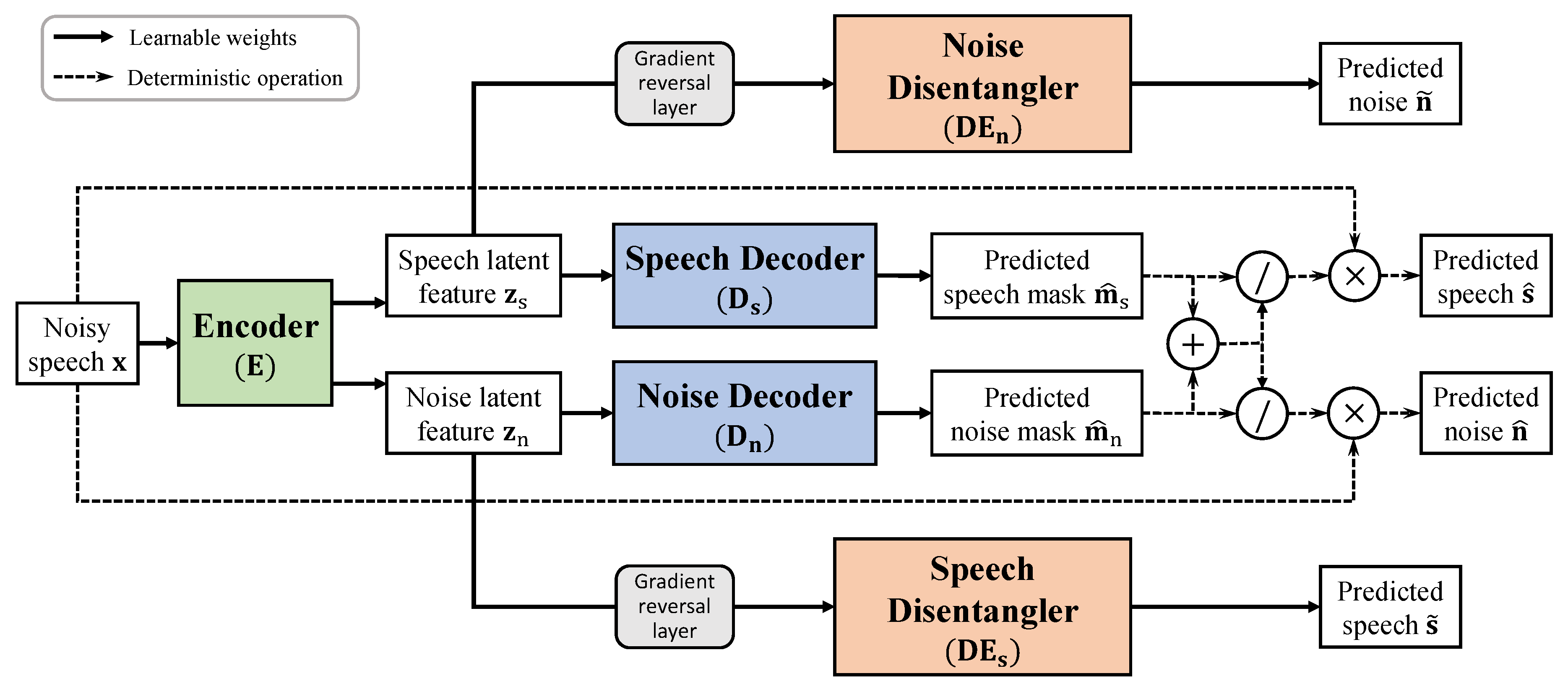
Figure 1. The architecture of the proposed model for disentangled feature learning.
Applsci 09 02289 g001
Figure 2. Plot of losses on training the proposed model.
Applsci 09 02289 g002
Figure 3. The architectures of the baseline models.
Applsci 09 02289 g003
Figure 4. (From top to bottom) The spectrograms of noisy speech degraded by metro noise with 3 dB signal-to-noise ratio (SNR), enhanced speech by the s n T model, enhanced speech by the s n D T model, and the corresponding clean speech, respectively.
Applsci 09 02289 g004
Figure 5. Results of subjective preference test ( % ) comparing the speech quality for the s n T and s n D T models with various SNR values.
Applsci 09 02289 g005
Figure 6. Variances of perceptual evaluation of speech quality (PESQ) scores for the 14 different noise types in various SNR environments.
Applsci 09 02289 g006
Figure 7. Visualization of speech latent feature ( z s ) using t-distributed stochastic neighbor embedding (t-SNE) in the matched noise condition.
Applsci 09 02289 g007aApplsci 09 02289 g007b
Figure 8. Visualization of speech latent feature ( z s ) using t-SNE in the mismatched noise condition.
Applsci 09 02289 g008
Table 1. Results of perceptual evaluation of speech quality (PESQ), segmental signal-to-noise ratio (segSNR), extended short-time objective intelligibility (eSTOI), and signal-to-distortion ratio (SDR) values of the proposed and baseline networks in the matched noise conditions, where 6 and 9 dB cases are unseen SNR conditions.
(a) PESQ(b) segSNR
SNR (dB) noisy sT snT nDT snDT SNR (dB) noisy sT snT nDT snDT
−61.532.002.122.062.22−6−6.871.493.182.853.53
−31.712.232.352.302.45−3−5.393.064.313.934.92
01.902.442.572.522.660−3.654.575.585.276.29
32.112.642.762.722.853−1.806.087.036.797.86
62.332.832.952.903.0260.327.418.338.149.20
92.542.993.103.053.1792.578.649.569.3810.43
Aver.2.022.522.642.592.73Aver.−2.475.216.336.067.04
(c) eSTOI(d) SDR
SNR (dB) noisy sT snT nDT snDT SNR (dB) noisy sT snT nDT snDT
−60.440.560.590.570.61−6−5.977.077.967.228.75
−30.520.640.670.650.69−3−3.119.6310.429.8511.10
00.590.710.740.730.760−0.1711.9212.6712.1613.21
30.670.770.800.790.8232.8014.0614.7114.2715.14
60.740.820.840.840.8665.7815.8116.4216.0316.81
90.800.860.880.870.8998.7817.3417.9417.5618.24
Aver.0.630.730.750.740.77Aver.1.3512.6413.3512.8513.88
Table 2. Results of PESQ, segSNR, eSTOI, and SDR values of the proposed and baseline networks in the mismatched noise conditions, where 6 and 9 dB cases are unseen SNR conditions.
(a) PESQ(b) segSNR
SNR (dB) noisy sT snT nDT snDT SNR (dB) noisy sT snT nDT snDT
−61.331.681.771.791.90−6−6.59−0.861.781.701.90
−31.551.932.022.022.13−3−5.080.812.852.722.81
01.772.162.252.272.350−3.352.583.503.474.04
31.982.382.462.442.553−1.484.164.974.895.69
62.202.592.672.652.7560.645.826.646.607.44
92.412.782.862.832.9392.917.298.118.088.97
Aver.1.882.252.342.332.43Aver.−2.163.304.644.585.14
(c) eSTOI(d) SDR
SNR (dB) noisy sT snT nDT snDT SNR (dB) noisy sT snT nDT snDT
−60.390.460.480.480.51−6−6.001.962.442.202.59
−30.470.550.580.570.60−3−3.114.895.375.215.57
00.550.630.660.660.680−0.177.898.378.268.61
30.630.710.740.730.7532.7910.5010.9210.7811.17
60.710.770.800.800.8165.7813.0113.4113.2413.66
90.780.820.840.840.8698.7815.1115.5215.3715.82
Aver.0.590.660.680.680.70Aver.1.348.899.349.189.57