Abstract
In this study, the issues of complicated interactions between process variables were solved by decoupling techniques; in particular, simplified decoupling was used due to its simplicity and robustness. A new approach to solving decoupling realizability was developed by using the modified particle swarm optimization (PSO) algorithm. However, time delays still existed in the diagonal elements of the decoupled matrix, and they resulted in a more sophisticated controller design and sluggish responses in the outputs. To overcome the adverse effects of time delays, a Smith predictor, also known as a dead time compensator, is normally used. In this work, a Smith predictor structure in combination with simplified decoupling for multivariable processes was proposed in order to enhance system performances in terms of the servomechanism problem. The proportional integral or proportional integral derivative (PI/PID) controller tuning rules for several common industrial processes, such as first-order, second-order, and second-order with negative zero systems, were obtained. Many multivariable industrial processes were adopted to simulate the effectiveness of the proposed method in terms of the servomechanism problem and robust response.
1. Introduction
Multivariable processes with multiple time delays are common in most industrial systems. For such systems, interactions between process variables cause difficulties in feedback controller design. Most advanced control strategies deal with that kind of problem by two different approaches: decentralized and centralized control. To design a decentralized control, most control engineers normally adopt traditional single-loop PID controllers for multivariable systems, known as multi-loop PI/PID controllers, because of their simplicity, effectiveness, and easy implementation [1,2,3]. However, they only work well for modest interactive processes. In systems with strong interactions between channels, centralized control is advisable. Its scheme can be classified into two kinds: a decoupling network in combination with a diagonal matrix controller [4,5,6] or a pure centralized strategy [7,8,9]. In this work, therefore, the centralized control with the decoupling network is addressed to convert a multi-input multi-output (MIMO) system into a multi-loop single-input single-output (SISO) system and conventional design approaches are used to control the whole system.
In practice, simplified decoupling is the favorite choice because of its simple decoupling network, the unitary diagonal elements, and robustness [4,5]. When solving decoupling problems, one has to approximate very complicated transfer functions to some standard forms and also deal with realizability issues, which are a major cause of improper (non-causal) transfer functions [5,6,7,10,11,12]. Numerous approximation techniques or reduced-order models are available, such as the prediction error method (PEM), the least-squares algorithm, the linear least-squares approximation [7] or Gaussian approach in the frequency domain, and the coefficient matching (CM) method [2,5]. However, the major disadvantage of these mentioned method is the computational burden when the order of MIMO systems increases. In this work, the particle swarm optimization (PSO) algorithm was adopted to approximate the complicated functions of decoupling elements to some well-known forms of industrial processes, such as first-order plus time delay (FOPTD), second-order plus time delay (SOPTD), and second-order plus time delay with negative zero (SOPTDNZ) systems. A minor modification was proposed to handle the improper transfer functions which may be obtained from the proposed algorithm.
However, time delays still exist in the diagonal elements of the apparent decoupled matrix. It is obvious that processes with significant dead time are hard to analyze and design based on standard feedback controllers and also result in sluggish responses in outputs. The Smith predictor (SP) scheme, known as the dead time compensator (DTC), is an appropriate method to deal with this situation by removing the delay terms from the closed-loop transfer functions [13]. However, the original scheme is only applied for SISO systems with their controllers tuned for a tradeoff between robustness and performance. To overcome this drawback, many variations of the SP have been proposed, and the most frequently used structure is a first-order lag filter (FOLF) on the feedback loop, also called the filter Smith predictor (FSP) [14,15]. From this method, the DTC structure can handle integrating and unstable processes [16,17]. In addition, other scholars have also extended this scheme to MIMO cases as well [18,19,20,21,22,23].
In order to expand the SP to MIMO systems, two approaches normally can be used. The first one is an FSP structure which is applied directly to the whole multivariable system [18,19,21,22]. The second one is done in combination with decoupling techniques which simplify the transfer function matrix of processes and then address an SP scheme for each single loop like that of SISO systems [20]. In the present work, the latter was adopted by using the simplified decoupling technique and the original SP for the sake of simplicity. The great advantage of this combination is that it completely removes delay terms out of the diagonal elements of the decoupled apparent matrix. Therefore, a delay-free part can be used for feedback controller design. In some cases, however, the first-order lag filter, if needed, would be put behind the PI/PID controllers to improve the tracking performance as well as robustness.
It is well known that the internal model control (IMC) method [23] is very effective for the design of PI/PID controllers. In this paper, a general form of controllers is presented, including a PI/PID controller and a FOLF in series [2,3]. The proposed method is based on the direct synthesis approach in which the primary PI/PID controllers are designed based on the desired closed-loop transfer functions [24]. Due to the properties of the SP structure, only the delay-free parts of the diagonal elements of the decoupled apparent matrix were addressed when designing the multiloop PI/PID controllers. Consequently, the resulting analytical tuning rules were derived for some common industrial processes. In order to evaluate the robustness of the controllers, the structure was performed in the presence of diagonal multiplicative output uncertainty [23,25,26].
This paper is organized as follows. Section 2 briefly introduces the simplified decoupling Smith predictor structure for multivariable processes; the approximation method by using the modified PSO algorithm is also addressed to reduce the order of process models and solve the issues of realizability of the simplified decoupling technique. Further, the IMC-PI/PID approach for controller tuning rules of some common industrial processes are presented, and the performance and robustness of the proposed control strategies are also discussed in this section. Some case studies are illustrated by simulations in Section 3. Finally, conclusions are given in Section 4.
2. Materials and Methods
2.1. Simplified Decoupling Smith Predictor Structure
Consider an n-input and n-output open-loop multivariable process with the general transfer function matrix for stable, square, and multidelays, which is represented by the following matrix:
where , of which denotes the physically proper, stable, and delay-fee transfer function. represents the time delay.
The multivariable Smith predictor control scheme is shown in Figure 1, where and are the process and its model, respectively. is also the process model but all the delays have been eliminated. is the primary controller of the following form:
The closed-loop transfer function matrix from set-points to outputs becomes
When the model is perfect, , and Equation (3) is rewritten as
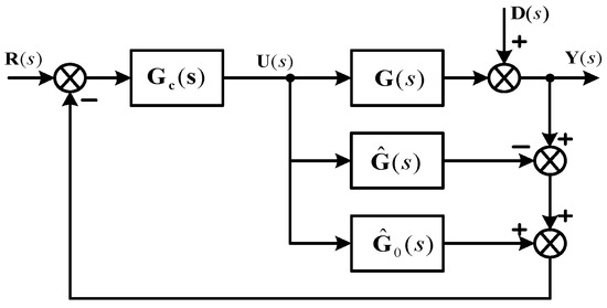
Figure 1.
Block diagram of multivariable Smith predictor (SP) control.
The time delay terms have been removed from the denominators of the closed-loop system transfer matrix. Similarly, there are no delay terms in the transfer function matrix from disturbances to outputs, and when the model is perfect, (). Therefore, the primary controller can be designed for the delay-free part and it is the main attractiveness of this control scheme. Equation (4) can be rewritten as follows:
where is the closed-loop transfer matrix corresponding to the designed controller of the delay-free part.
It can be seen that the actual system performances could not be guaranteed because of the part in Equation (5), regardless of how good the performance of is. In special cases where all delay terms of each row of the transfer function matrix are identical, can be rewritten by . Consequently, and the system outputs are the delayed outputs of ; that is, to some extent, the system performance and robustness still meet requirements. In most cases, however, this desired property is not preserved. In order to overcome this problem and improve the performance of the multivariable Smith predictor control system, a decoupling Smith predictor (DSP) system was proposed (Figure 2), where is a decoupling matrix for the system transfer function matrix , is the decoupled process, and . is the same as except that all the delays are removed. It is obvious that the and will be diagonal matrices due to the properties of decoupling techniques. Therefore, the problem of controller design for multivariable systems with multiple time delays is simplified to multiple single-loop Smith predictors and various simple methods can be utilized to design the control systems.
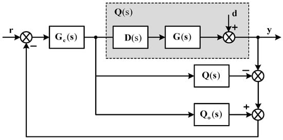
Figure 2.
Decoupling SP (DSP) control system.
The decoupling techniques are available for ideal, simplified, and inverted decoupling [4]. However, in this study, simplified decoupling was chosen because of its robustness and simple decoupling network (i.e., the diagonal elements of the decoupling matrix, , were set as unity) [4,5]. Truong and Lee proposed an extended method of simplified decoupling for general forms of a MIMO case where the decoupled apparent processes are given as follows [5]:
where , for which is the transpose of its cofactor matrix; and , for which is the Hadamard or Schur product of element-by-element multiplication.
Using Equation (6), the decoupler elements for some typical processes were obtained and are summarized in Table 1.

Table 1.
The matrix elements of the simplified decoupler for 2 × 2 and 3 × 3 processes.
The diagonal elements of the decoupled process are also expressed in Table 2. It is obvious that each element is complicated and incapable of serving in analysis and design problems. A CM method using Maclaurin series expansion was proposed by Truong to reduce the decoupled transfer functions into some standard forms and solve the problems of decoupler realizability as well [5]. The greatest disadvantage of that method is the burden of algebraic computations when the order of MIMO systems increases. Therefore, in this work, a novel approach to deal with these issues of simplified decoupling was proposed by using the modified PSO algorithm [27,28,29].
Table 2.
The diagonal elements of the decoupled matrix for 2 × 2 and 3 × 3 processes.
2.2. The Modified PSO Algorithm for Model Reduction
The concept of PSO was developed based on the social behavior of swarms looking for the most fertile feeding location [27]. All solutions in PSO can be represented as particles in a swarm. Each particle has a position in a search space which represents a parameter value and a velocity vector used to update new positions. At each step, all particles are updated with the two best solution values: personal best position (Pbest) so far and global best position (Gbest) (i.e., the best value obtained among all particles up to that step). The well-known update equations of position and velocity of each particle are as follows:
where and are the velocity and position of the ith particle, respectively; t, iteration, , and are acceleration (scaling, learning) factors; and are real numbers generated randomly in the (0–1) range; is the inertial weight; and M is the maximum number of iterations.
In this work, the following form of the transfer function, Equation (11), was used as a general approximated model for the sake of simplicity. Apparently, a higher-order transfer function could be developed to obtain a better approximation for diagonal elements of a decoupled matrix, but it would make it difficult to derive an analytical PID controller. Moreover, based on reviewing related publications in the process control field, Equation (11) was found to be suitable for most process applications. Further, in this study, it can address equivalent models for the decoupler elements () and the diagonal elements of the decoupled process () shown in Table 1 and Table 2.
where are time constants which should be positive values, assuming ; is gain; and is a non-negative parameter. When , the model, Equation (11), becomes the popular SOPTD system, Equation (16), or even the FOPTD system, Equation (15), if the smaller time constant of the system is also equal to zero. is a delay time, and in order to facilitate the approximation procedure, it is a predetermined value based on the unit step response of the original model.
The parameters that need to be tuned are written in the following vector form:
The different constraints of these parameters are defined as
where are determined based on the open-loop unit step responses of the original model.
The structure of the approximation algorithm is illustrated in Figure 3. This structure can work for both open-loop and closed-loop systems. In this work, a unit step input was applied to the open-loop system, which was always stable. However, in case the open-loop system was unstable, a simple feedback controller such as a proportional control was adopted to make the closed-loop systems stable. Then, the proposed method could be applied normally.
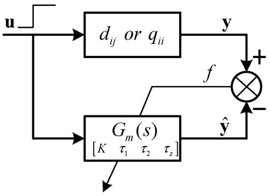
Figure 3.
Structure of the approximation algorithm.
The gain constraints and other boundaries of time constants could be determined based on the step response of the system. These pairs of input–output data were recorded and adopted for the training algorithm as well. The fitness function was calculated by
At each step of velocity and position update, the improperness of a reduced-order model is always apparent. If there are any violations due to any particle positions, new positions would be created randomly. The proposed modified PSO algorithm was used here to solve the realizability problem of the simplified decoupler. The flow chart of the proposed algorithm is shown in the Figure 4.
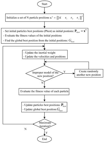
Figure 4.
The flow chart of the proposed particle swarm optimization (PSO) algorithm.
The purpose of using the PSO algorithm was to propose a method for finding an approximation transfer function of a complicated system. After utilizing the reduction technique to approximate the complex dynamics of decoupling elements into appropriate lower-order models, most industrial processes normally have some standard forms, such as FOPTD, SOPTD, and SOPTDNZ systems, given as Equations (15)–(17), respectively:
It is obvious that time delays still exist in the diagonal elements of a decoupled matrix which result in sluggish responses in the outputs. In this work, Smith predictors were adopted to overcome this issue, and as mentioned above, the delay terms were also eliminated from the closed loops. As a result, we could use various methods to design multi-loop controllers for multi-loop delay-free systems (18–20); that is, could be removed from Equations (15)–(17) when designing the controllers:
2.3. IMC-PI/PID Approach for Controller Design
The multivariable Smith predictor is based on the multiple single-loop Smith predictor control design. Let the primary controller be as in Equation (2), and then, each diagonal controller has the standard form of the PID controller in series with the FOLF:
The was designed with respect to the delay-free part of such that the closed-loop system formed by and had the desired performance. Figure 5 shows block diagrams of feedback control strategies, including the classical feedback control and the internal model control as well [24]. Note that, in this case, the controlled plant is a delay-free transfer function.
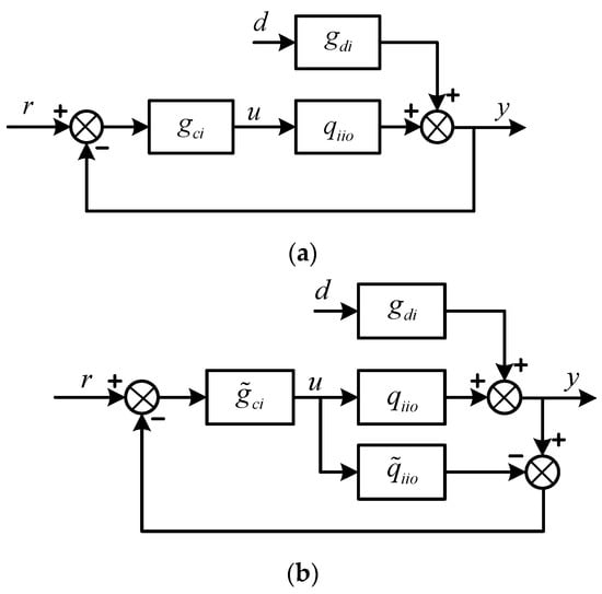
Figure 5.
The one-degree-of-freedom feedback control diagram: (a) classical feedback control; (b) internal model control.
According to the IMC theory, the process models are factored into two parts:
where contains delay time terms and/or right half plane (RHP)zeroes and . According to Equations (18)–(20), .
Generally, the IMC controller is designed as
The term is called the IMC filter and normally has the following form:
There are some criteria used to choose the appropriate value of which can be found in the available literature. For example, Skogestad (2003) suggested choosing to be equal to the time delay of the process. However, in this work, was an adjustable parameter which controlled the tradeoff between performance and robustness; was the relative order and had to be large enough to make the IMC controller (semi)proper; and was chosen to cancel the jth unstable poles in the process model.
Therefore, the ideal feedback controller for achieving the desired loop responses can be easily obtained by
The resulting controller given by Equation (26) normally does not have the standard PI/PID controller form despite it being physically realizable. To take advantage of an available commercial PID controller, it must be converted into the equivalent PID type. In this case, it is necessary to utilize some approximation techniques. In this paper, Maclaurin expansion was used to approximate a PID controller for some typical industrial processes such as the transfer functions (18–20).
Since the feedback controller has the offset-free integral term, can be rewritten as
The rational approximation form of Equation (26) can be found by expanding in a Maclaurin series [1,2,5]:
2.4. IMC-PI/PID Tuning Rules for Typical Processes without Time Delay
In this work, three free-delay process models were considered:
Case 1: The first-order system:
The proposed IMC filter structure
The ideal feedback controller is obtained by
Therefore, in this case, the PI controller settings are obtained:
Note that, in this case, .
Case 2: The second-order system:
The proposed IMC filter structure
The ideal feedback controller is obtained by
Rewriting Equation (36) into the form of Equation (21), the controller is obtained as Equation (37):
Therefore, the setting rules of the controller are obtained:
Case 3: The second-order with negative zero:
The proposed IMC filter structure
The ideal feedback controller is obtained by
The ideal controller (44) does not have the standard form of Equation (21). Therefore, it was necessary to use the approximate techniques according to Equation (28), and the setting rules were derived as follows:
The tuning rules for different types of process models are summarized in Table 3.
Table 3.
Tuning rules for different types of delay-free process models.
2.5. System Performance and Robustness Analysis
2.5.1. Integral Absolute Error (IAE) Index
To evaluate the closed-loop performance, the IAE criterion was considered, which is defined as
where is a finite time which is chosen for the integral approach steady-state value.
2.5.2. Total Variation (TV)
To evaluate the magnitude of the manipulated input usage, the total up and down movement of the control signal was considered as
TV is a good measure of the smoothness of controller output and should be small [2,5,25].
2.5.3. Robust Stability Analysis
The robustness of a control system is one of the most important issues in any controller design. The dynamics of real plants usually have many sources of uncertainty, which cause poor performance or even instability in the control systems. In this paper, the robust stability was studied by considering the multiplicative output uncertainty in each loop of the diagonal element of the decoupled matrix, as shown in Figure 6. It can be expressed as follows:
where , and denotes a normalized perturbation with norm less than 1 (); is the nominal decoupled plant model; denotes the set of possible perturbed process models; and is the diagonal decoupled transfer, which is considered as the function of the perturbation of its nominal model due to uncertainty in the multiplicative output .
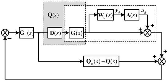
Figure 6.
DSP structure with multiplicative output uncertainty.
The structure of the DSP structure is shown in Figure 7 where the transfer function matrix from the outputs to the inputs of can be determined by
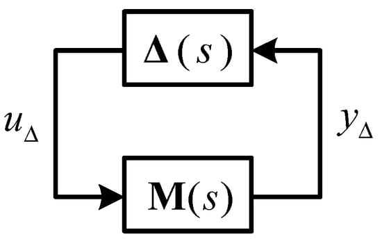
Figure 7.
structure for robustness analysis.
According to the synthesis, the control system will remain stable under multiplicative output uncertainty if the following constraint inequality is satisfied:
3. Results
In this section, three examples are considered to demonstrate the performances of the proposed method in comparison with those of other well-known methods.
Example 1.
Wood and Berry (WB) distillation column.
The WB column is one of the most representative two-input two-output (TITO) process models widely used for evaluating the performance of the multi-loop controllers. The original matrix transfer function of WB can be found in [30] and expressed as Equation (54):
The matrix elements of the simplified decoupler for a 2 × 2 process can be calculated by the equations in Table 1:
Therefore, the simplified decoupling matrix can be easily obtained:
For the purpose of controller design, the diagonal elements of the decoupled matrix must be calculated by the equations in Table 2 for a 2 × 2 case:
Since it is impossible to design an analytical PID controller based on these equations, the modified PSO algorithm presented in Section 2 was adopted in order to reduce in Equations (58) and (59) to the standard form of Equation (11). The approximation procedure of is as follows:
- Step 1:
- Plotting the step response of (Figure 8) and recording its output for training.
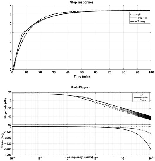 Figure 8. Step and Bode responses of original q11 and its approximations (Wood and Berry (WB) column).
 - Step 2:
- Based on the step response, the constraints of the tuned parameters in Equation (11) are predetermined, including .
- Step 3:
- Running the proposed PSO algorithm according to Figure 4 to find the best approximation.
It is similar for the approximation of . The obtained results are the following equations:
Figure 8 and Figure 9 also illustrate the comparison of the responses of approximation models of the proposed method with the CM method of Truong and Lee [5] in time and frequency domains. It can be seen that the step responses of the solution transfer functions using PSO were better approximated; that is, they were as close as possible to the step responses of the original models. Further, the fitness function, Equation (14), guaranteed the minimum error of these two outputs. Actually, the purpose of using the PSO algorithm was to propose a novel and simple approach to seeking approximation models with effortless computation. The proposed method cannot guarantee the optimal solution but it is easy to implement in applications.
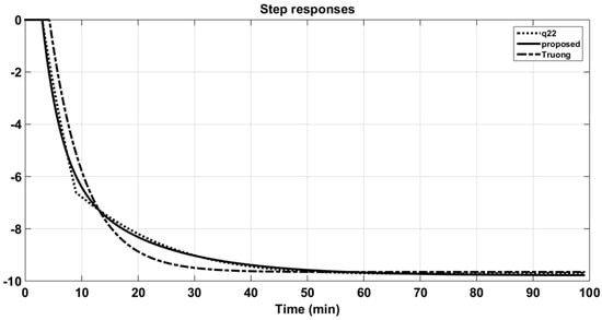
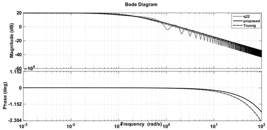
Figure 9.
Step and Bode responses of original q22 and its approximations (WB column).
The implementing diagram of the DSP structure is shown in Figure A1, Appendix A. The performance of the proposed method was also compared with those of existing design methods such as simplified decoupling [5], the decentralized control of Wang et al. [31], and the simplified filtered Smith predictor [21]. The sequential unit step changes in the set-points were made to the first and second loops, respectively. The robust stability was examined for all of the comparative design methods by using Equation (53).
The resulting controller parameters and performance indices are listed in Table 4. The closed-loop responses to the set-point changes, the control signals of loops 1 and 2, and the structured singular values (SSV) plots for robust stability are shown in Figure 10a,b, Figure 11a,b and Figure 12, respectively. It is apparent from the table and figures that the proposed controller provided superior performance.
Table 4.
Controller parameters and resulting performance indices for the WB column.
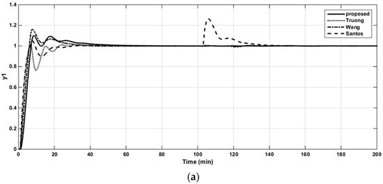
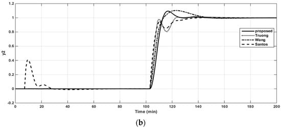
Figure 10.
Closed-loop responses to the unit step changes in the set-point of loop 1 (a). Closed-loop responses to the unit step changes in the set-point of loop 2 (b).
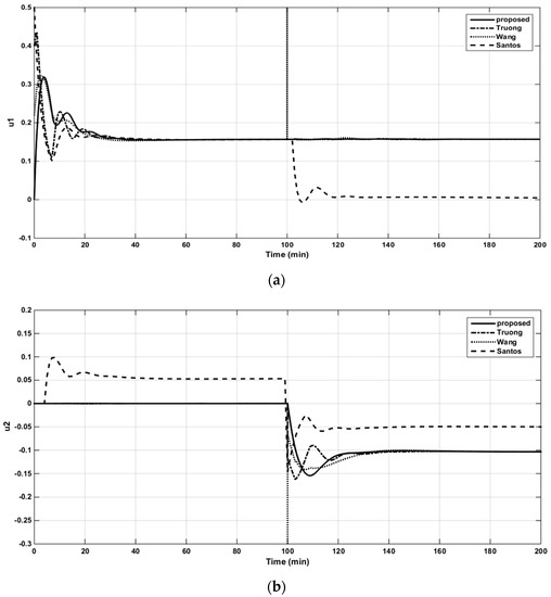
Figure 11.
The control signal in loop 1 of the WB column (a). The control signal in loop 2 of the WB column (b).
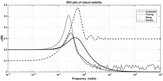
Figure 12.
The SSV plots for robust stability in the WB column.
The robustness of the controller was evaluated by inserting the perturbation uncertainties of ±10% and ±20% in the process gain, time constant, and time delay into the actual process, simultaneously, whereas the controller settings were those provided for the nominal process. The simulation results of the model mismatch for various tuning methods of two cases are given in Table 5 and Table 6, respectively. In the first case (±10%), the responses of all tuning methods were still stable, but the proposed method had the best performance in general. In the latter (±20%), however, the responses of Truong’s and Wang’s methods became unstable, while Santos et al.’s method and the DSP structure still gave acceptable results. However, Table 6 shows that it is obvious that the proposed method had the better performance.
Table 5.
Robustness analysis for the WB column under ±10% parametric uncertainty in all parameters.
Table 6.
Robustness analysis for the WB column under ±20% parametric uncertainty in all parameters.
Example 2.
Vinante and Luyben (VL) column.
The transfer function matrix for a VL column introduced by Luyben [32] has the following form:
This plant was chosen to evaluate the proposed method because of the special case in . According to Table 1, is a non-causal element (), which means it cannot satisfy the realizability problem. In this case, the steady state gain, , of this element can be used instead. The simplified decoupling matrix can be easily obtained by using Table 1 (2 × 2 process):
Similar to Example 1, the modified PSO algorithm in Section 2 was adopted in order to reduce to the standard form of Equation (11). The obtained results are the following equations:
The step responses of the elements of the diagonal decoupled matrix and their approximations are shown in Figure 13 and Figure 14. Their Bode plots of magnitude and phase are also compared. It can be seen that the proposed method had better approximation when compared in the phase plot.
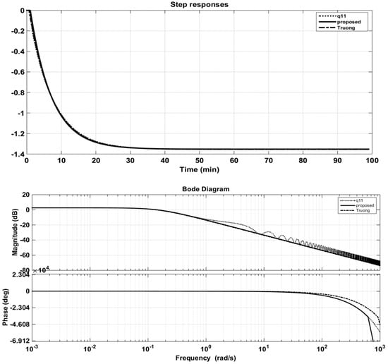
Figure 13.
Step and Bode responses of original q11 and its approximations (Vinante and Luyben (VL) column).
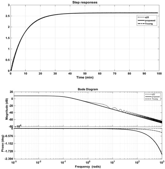
Figure 14.
Step and Bode responses of original q22 and its approximations (VL column).
In this simulation study, the performance of proposed method was compared with the simplified decoupling method (Truong and Lee [5]) as well as the centralized inverted decoupling method (Garrido et al. [8]). The implementing diagram for VL column is shown in Figure A2, Appendix A. The resulting multi-loop PID controllers by the proposed and other methods were tabulated and are shown in Table 7. For the sequential unit step changes in the set-points, Figure 15a,b compare the closed-loop time responses afforded by the proposed and other methods. The proposed controller showed superior responses with faster settling times and no overshoots compared with the other methods. The sequential unit step changes considered as disturbances were also investigated for the first and second loops. The values of the performance indices (Table 7) confirmed the superior performance of the proposed controller for the load changes as well as the set-point changes. The control signals of the two loops are presented in the Figure 16a,b.
Table 7.
Controller parameters and resulting performance indices for the VL column.
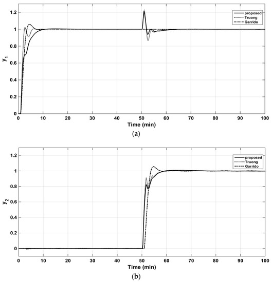
Figure 15.
Closed-loop responses to the unit step changes in the set-point of loop 1 (VL column) (a). Closed-loop responses to the unit step changes in the set-point of loop 2 (VL column) (b).
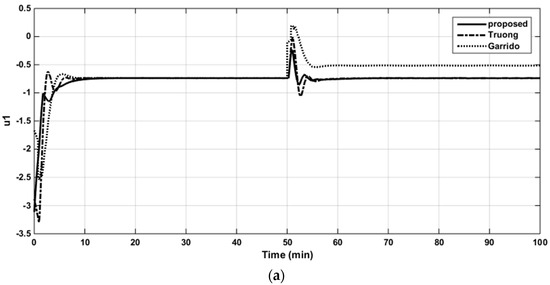
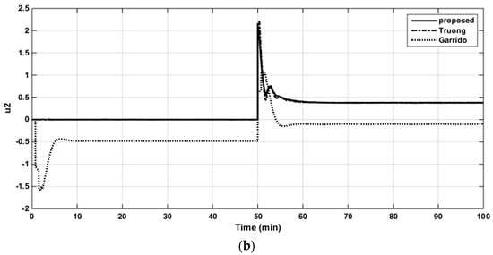
Figure 16.
The control signal in loop 1 of the VL column (a). The control signal in loop 2 of the VL column (b).
For the robustness study, the SSV analysis is illustrated in Figure 17 and the perturbation uncertainties of ±20% were inserted in all three parameters (time constants, gain, and time delay) of the nominal model, simultaneously. As shown in Table 8, the controller settings of the proposed method provided superior robust performance compared with the others.
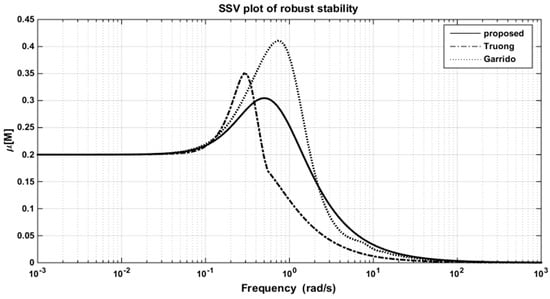
Figure 17.
The SSV plots for robust stability in the VL column.
Table 8.
Robustness analysis for the VL column under ±20% parametric uncertainty in all parameters.
Example 3.
Ogunnaike and Ray (OR) column.
A well-known multiproduct distillation column for the separation of a binary ethanol–water mixture studied by many researchers was considered [5,33]. The open-loop transfer function matrix is given by Equation (66):
Using Table 1 for the 3 × 3 case, it can be seen that the equations for calculations of were quite complex and that it was not as easy to directly derive the decoupler matrix as the two previous examples. In this case, the proposed PSO algorithm was also used as described step by step in Example 1 to obtain each element of the decoupler matrix. The final obtained result was as follows:
Then, using Table 2 and the proposed approximation technique, the diagonal matrix of the decoupled process was derived according to the following equations:
From Figure 18, Figure 19 and Figure 20, it can be concluded that the proposed approximation would give better results if the size of the system were increased.
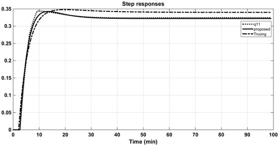
Figure 18.
Step responses of the original q11 and its approximations (Ogunnaike and Ray (OR) column).
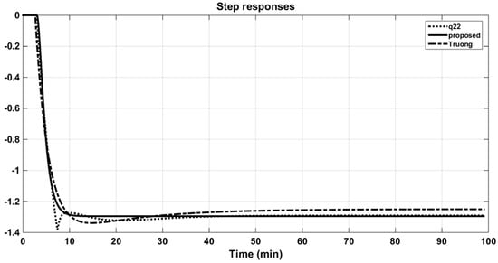
Figure 19.
Step responses of the original q22 and its approximations (OR column).
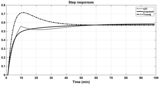
Figure 20.
Step responses of the original q33 and its approximations (OR column).
In this case, the proposed method was compared with those of decentralized control with multi-loop PI/PID controllers [2] and simplified decoupling [5]. The implementing diagram for OR column is shown in Figure A3, Appendix A. In the simulation, the sequential step changed in the set-points of loops 1–3, and from the results (Figure 21a–c), one can see that the proposed controller had faster rising and settling responses than those of the others. Disturbance rejection performance was also evaluated by considering the mutual effects of sequential changes on loops 1–3. In Figure 21a–c, it is clear that the proposed controller gave the least effect (i.e., lowest in the magnitudes of variations and fastest recovering times). The control signals of the three loops are presented in the Figure 22a–c. The resulting controller parameters together with the performance indices are summarized in Table 9.
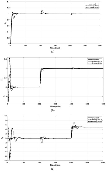
Figure 21.
Closed-loop responses to the unit step changes in the set-point of loop 1 (OR column) (a). Closed-loop responses to the unit step changes in the set-point of loop 2 (OR column) (b). Closed-loop responses to the unit step changes in the set-point of loop 3 (OR column) (c).
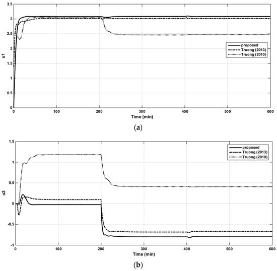
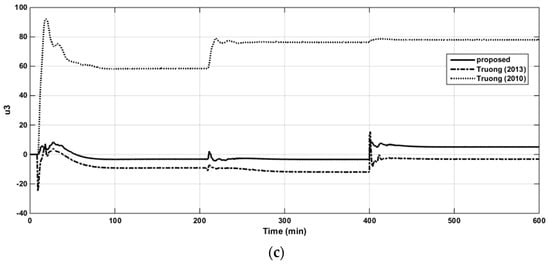
Figure 22.
The control signal in loop 1 of the OR column (a). The control signal in loop 2 of the OR column (b). The control signal in loop 3 of the OR column (c).
Table 9.
Controller parameters and resulting performance indices for the OR column.
The comparison of the structured singular values for robust stability of the proposed and other methods is illustrated in Figure 23. In addition, to demonstrate the robust performance of the proposed method, a simulation study was also done by inserting the perturbation uncertainties of ±20% in all three process parameters. The simulation results for the plant–model mismatch were tabulated and are shown in Table 10. As seen from the table, the proposed controller consistently afforded superior performance.
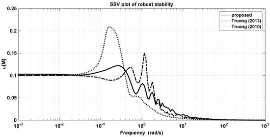
Figure 23.
The SSV plots for robust stability in the OR column.
Table 10.
Robustness analysis for the OR column under ±20% parametric uncertainties in all parameters.
4. Conclusions
In this paper, a new structure of a Smith predictor was proposed for multivariable systems by combining the SP with a simplified decoupling network. The general formulation of simplified decoupling was derived from previous works. However, in this study, the PSO algorithm was adopted to approximate model transfer functions and solve the problem of realizability. Multi-loop PI/PID controllers in series with first-order lag filters were used and the general tuning rules were also derived for the delay-free parts of some standard forms of industrial processes. The proposed approach is straightforward, easy to implement, and effective when the size of systems is increased. The time-domain simulations demonstrated the superior performance of the proposed structure with, fast and well-balanced closed-loop time responses for both the set-point and load changes. Robustness was investigated by SSV analysis in multiplicative output uncertainty. In order to guarantee robust stability, perturbation uncertainties of ±20% were inserted in all three process parameters, and the simulation results showed that the proposed method afforded superior robust performance in the plant–model mismatch case.
Author Contributions
The individual contributions of authors: conceptualization, T.N.L.V., V.L.C.; methodology, V.L.C., T.N.L.V.; writing of original draft preparation, V.L.C.; writing of review and editing, V.L.C., N.T.N.T.; supervision, J.H.J., T.N.L.V.; funding acquisition, J.H.J., T.N.L.V.
Funding
This research was supported by Ho Chi Minh City University of Technology and Education, and the “Human Resources Program in Energy Technology” of the Korea Institute of Energy Technology Evaluation and Planning (KETEP), with financial resources from the Ministry of Trade, Industry & Energy, Republic of Korea. [No. 20174030201760].
Conflicts of Interest
The authors declare no conflict of interest.
Appendix A
According to the proposed structure, the Simulink programs in Matlab are used to demonstrate the responses of the process systems in Example 1, 2 and 3. In this section, three block diagrams of the Simulink program are included
The block diagram of Simulink program in Example 1, WB column.

Figure A1.
The implementing diagram of the DSP structure for WB column.
Figure A1.
The implementing diagram of the DSP structure for WB column.

The block diagram of Simulink program in Example 2, VL column.

Figure A2.
The implementing diagram of the DSP structure for VL column.
Figure A2.
The implementing diagram of the DSP structure for VL column.

The block diagram of Simulink program in Example 3, OR column.

Figure A3.
The implementing diagram of the DSP structure for OR column.
Figure A3.
The implementing diagram of the DSP structure for OR column.

References
- Truong, N.L.V.; Lee, M. Analytical design of multi-loop PI controllers for interactive multivariable processes. J. Chem. Eng. Jpn. 2010, 43, 196–208. [Google Scholar]
- Truong, N.L.V.; Lee, M. Independent design of multi-loop PI/PID controllers for interacting multivariable processes. J. Process Control 2010, 20, 922–933. [Google Scholar]
- Nandong, J.; Zang, Z. Multi-loop design of multi-scale controllers for multivariable processes. J. Process Control 2014, 24, 600–612. [Google Scholar] [CrossRef]
- Gagnon, F.; Pomerleau, A.; Desbiens, A. Simplified, ideal or inverted decoupling. ISA Trans. 1998, 37, 265–276. [Google Scholar] [CrossRef]
- Truong, N.L.V.; Lee, M. An extended method of simplified decoupling for multivariable processes with multiple time delays. J. Chem. Eng. Jpn. 2013, 46, 279–293. [Google Scholar]
- Garrido, J.; Vázquez, F.; Morilla, F. An extended approach of inverted decoupling. J. Process Control 2011, 21, 55–68. [Google Scholar] [CrossRef]
- Garrido, J.; Vázquez, F.; Morilla, F. Centralized multivariable control by simplified decoupling. J. Process Control 2012, 22, 1044–1062. [Google Scholar] [CrossRef]
- Garrido, J.; Vázquez, F.; Morilla, F. Centralized inverted decoupling control. Ind. Eng. Chem. Res. 2013, 52, 7854–7866. [Google Scholar] [CrossRef]
- Vijay Kumar, V.; Rao, V.S.R.; Chidambaram, M. Centralized PI controllers for interacting multivariable processes by synthesis method. ISA Trans. 2012, 51, 400–409. [Google Scholar] [CrossRef]
- Xiong, Q.; Cai, W.J. Effective transfer function method for decentralized control system design of multi input multi-output processes. J. Process Control 2006, 16, 773–784. [Google Scholar] [CrossRef]
- Xiong, Q.; Cai, W.J.; He, M.J. Equivalent transfer function method for PI/PID controller design of MIMO processes. Process Control 2007, 17, 665–673. [Google Scholar] [CrossRef]
- Rajapandiyan, C.; Chidambaram, M. Controller design for MIMO processes based on simple decoupled equivalent transfer functions and simplified decoupler. Ind. Eng. Chem. Res. 2012, 51, 12398–12410. [Google Scholar] [CrossRef]
- Smith, O.J. Closed control of loops with dead time. Chem. Eng. Prog. 1957, 53, 217–219. [Google Scholar]
- Normey-Rico, J.E.; Camacho, E.F. Unified approach for robust dead-time compensator design. J. Process Control 2009, 19, 38–47. [Google Scholar] [CrossRef]
- Torrico, B.C.; Correia, W.B.; Nogueira, F.G. Simplified dead-time compensator for multiple delay SISO systems. ISA Trans. 2016, 60, 254–261. [Google Scholar] [CrossRef] [PubMed]
- Sanz, R.; Garcia, P.; Albertos, P. A generalized Smith predictor for unstable time-delay SISO systems. ISA Trans. 2018, 72, 197–204. [Google Scholar] [CrossRef] [PubMed]
- Lloyds Raja, G.; Ali, A. Smith predictor based parallel cascade control strategy for unstable and integrating processes with large time delay. J. Process Control 2017, 52, 57–65. [Google Scholar] [CrossRef]
- Seshagiri Rao, A.; Chidambaram, M. Smith delay compensator for multivariable no-square systems with multiple time delays. Comput. Chem. Eng. 2006, 30, 1243–1255. [Google Scholar]
- Tito, L.M.; Santos, R.; Flesch, C.C.; Normey-Rico, J.E. On the filtered Smith predictor for MIMO processes with multiple time delays. J. Process Control 2014, 24, 383–400. [Google Scholar]
- Garrido, J.; Vázquez, F.; Morilla, F.; Normey-Rico, J. Smith predictor with inverted decoupling for square multivariable time delay systems. Int. J. Syst. Sci. 2016, 47, 374–388. [Google Scholar] [CrossRef]
- Santos, T.L.M.; Torrico, B.C.; Normey-Rico, J.E. Simplified filtered Smith predictor for MIMO processes with multiple time delays. ISA Trans. 2016, 65, 339–349. [Google Scholar] [CrossRef] [PubMed]
- Rodríguez, C.; Normey-Rico, J.E.; Guzmán, J.L.; Berenguel, M. On the filtered Smith predictor with feedforward compensation. J. Process Control 2016, 41, 354–356. [Google Scholar] [CrossRef]
- Morari, M.; Zafiriou, E. Robust Process Control; Prentice Hall: Englewood Cliffs, NJ, USA, 1989. [Google Scholar]
- Seborg, D.E.; Edgar, T.F.; Mellichamp, D.A. Process Dynamics and Control; John Wiley & Sons: New York, NY, USA, 1989. [Google Scholar]
- Skogestad, S.; Postlethwaithe, I. Multivariable Feedback Control Analysis and Design, 1st ed.; John Wiley & Sons: New York, NY, USA, 1996. [Google Scholar]
- Sanchez-Pena, R.S.; Bolea, Y.; Puig, V. MIMO Smith predictor: Global and structured robust performance analysis. J. Process Control 2009, 19, 163–177. [Google Scholar] [CrossRef]
- Kennedy, J.; Eberhart, R. Particle swarm optimization. In Proceedings of the 1995 IEEE International Conference on Neural Networks, Nagoya, Japan, 4–6 October 1995; pp. 1942–1948. [Google Scholar]
- Guedria, N.B. Improved accelerated PSO algorithm for mechanical engineering optimization problems. Appl. Soft Comput. 2016, 40, 455–467. [Google Scholar] [CrossRef]
- Wang, D.; Tan, D.; Liu, L. Particle swarm optimization algorithm: An overview. Soft Comput. 2018, 22, 387–408. [Google Scholar] [CrossRef]
- Wood, R.K.; Berry, M.W. Terminal composition control of binary distillation column. Chem. Eng. Sci. 1973, 28, 1707–1717. [Google Scholar] [CrossRef]
- Wang, Q.G.; Huang, B.; Guo, X. Auto-tuning of TITO decoupling controllers from step tests. ISA Trans. 2000, 39, 407–418. [Google Scholar] [CrossRef]
- Luyben, W.L. Simple method for tuning SISO controllers in multivariable systems. Ind. Eng. Chem. Process Des. Dev. 1986, 25, 654–660. [Google Scholar] [CrossRef]
- Ogunnaike, B.A.; Lemaire, J.P.; Morari, M.; Ray, W.H. Advanced multivariable control of a pilot-plant distillation column. AIChE J. 1983, 29, 632–640. [Google Scholar] [CrossRef]


© 2019 by the authors. Licensee MDPI, Basel, Switzerland. This article is an open access article distributed under the terms and conditions of the Creative Commons Attribution (CC BY) license (http://creativecommons.org/licenses/by/4.0/).