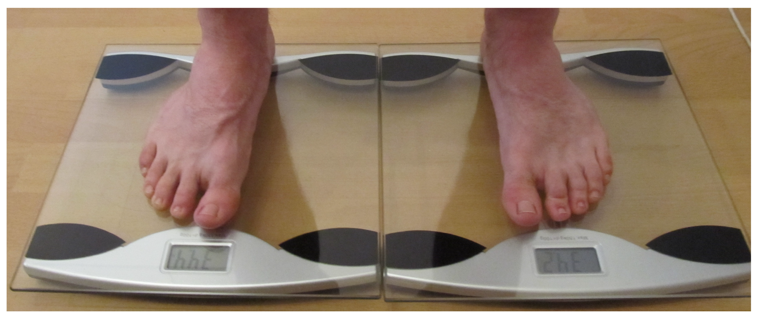
Figure 1.
Measuring leg load distribution by using two equal commercial scales.
Figure 1.
Measuring leg load distribution by using two equal commercial scales.
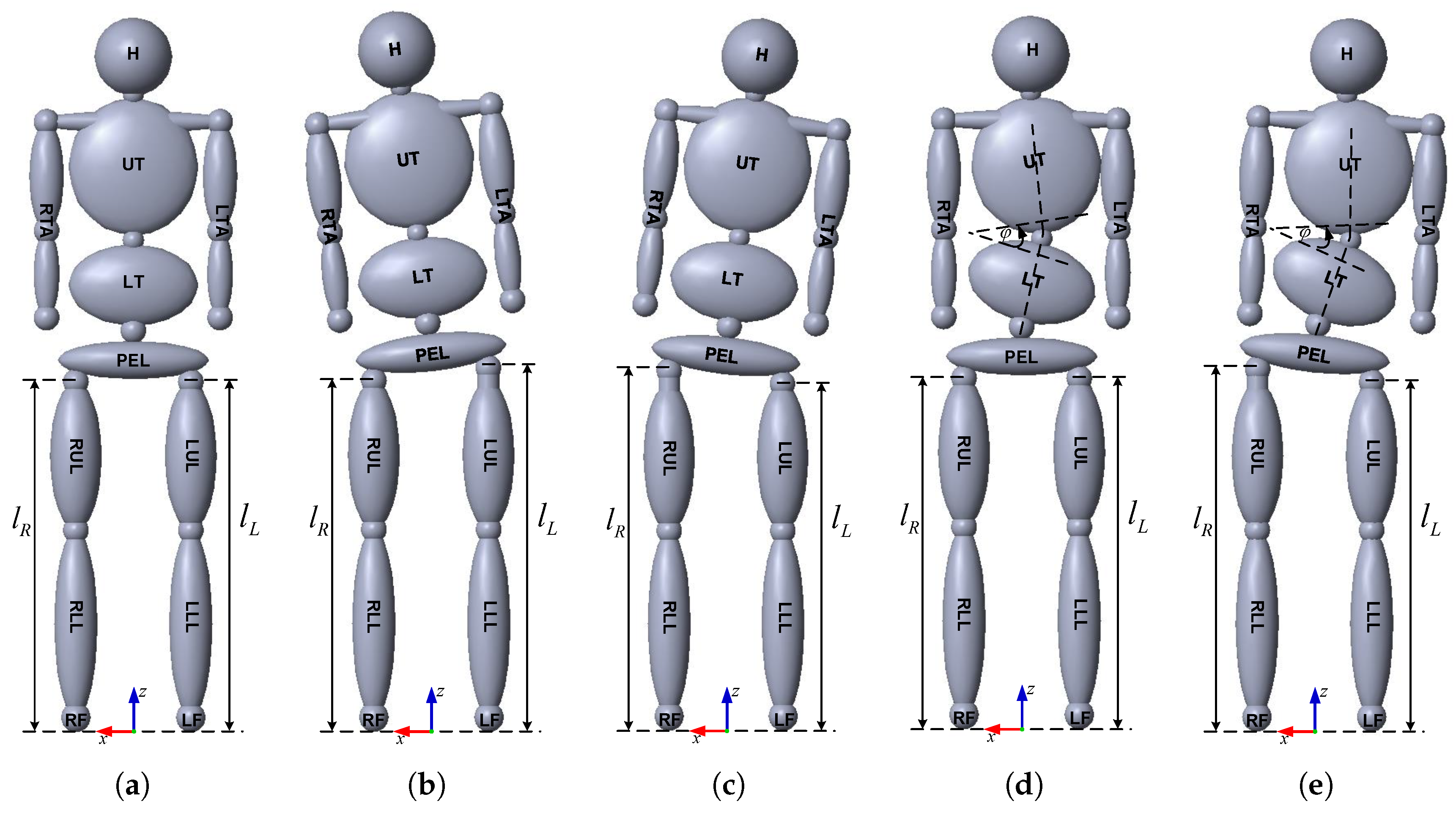
Figure 2.
12-segment anthropometric human body model with variable leg length and scoliosis (RF, Right Foot; LF, Left Foot; RLL, Right Lower Leg; LLL, Left Lower Leg; RUL, Right Upper Leg; LUL, Left Upper Leg; PEL, Pelvis; LT, Lower Trunk; UT, Upper Trunk; H, Head; RTA, Right Total Arm; LTA, Left Total Arm). Left leg length is given as , right leg length is , and the angle of scoliosis is : (a) human body without LLD and scoliosis (); (b) human body with LLD (); (c) human body with LLD (); (d) human body with scoliosis (); and (e) human body with LLD and scoliosis ().
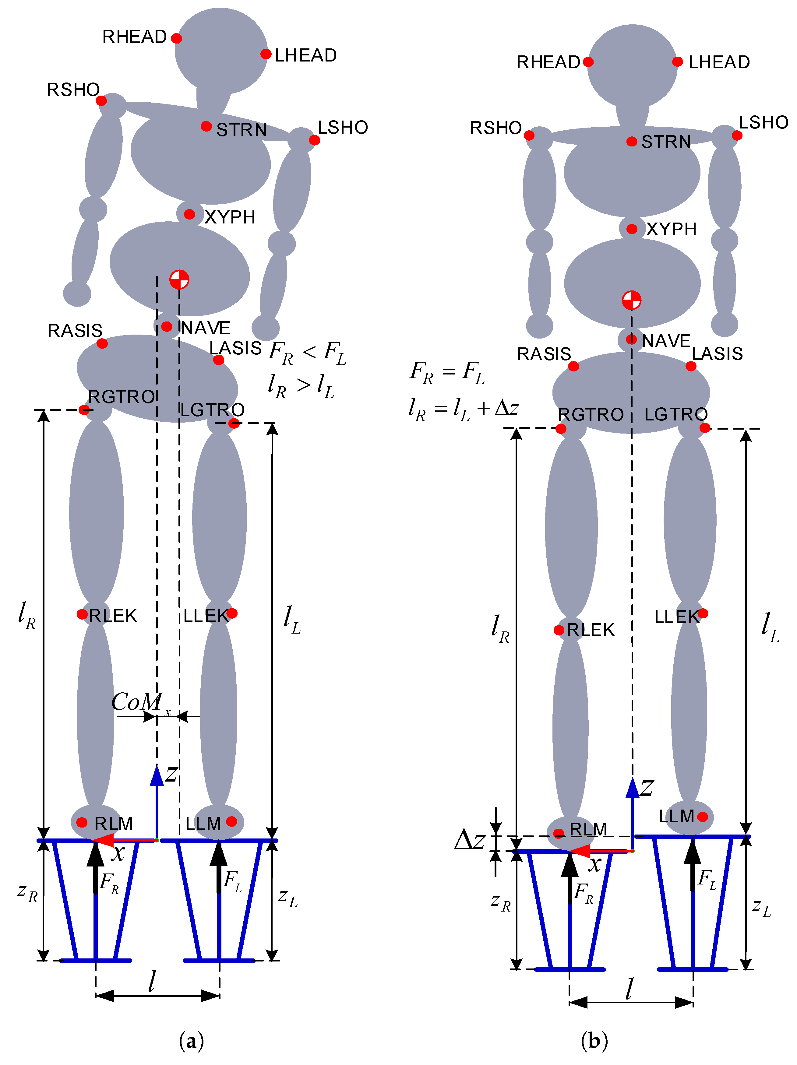
Figure 3.
Human Body Balancing: (a) human body with LLD (); and (b) balanced human body ().
Figure 3.
Human Body Balancing: (a) human body with LLD (); and (b) balanced human body ().
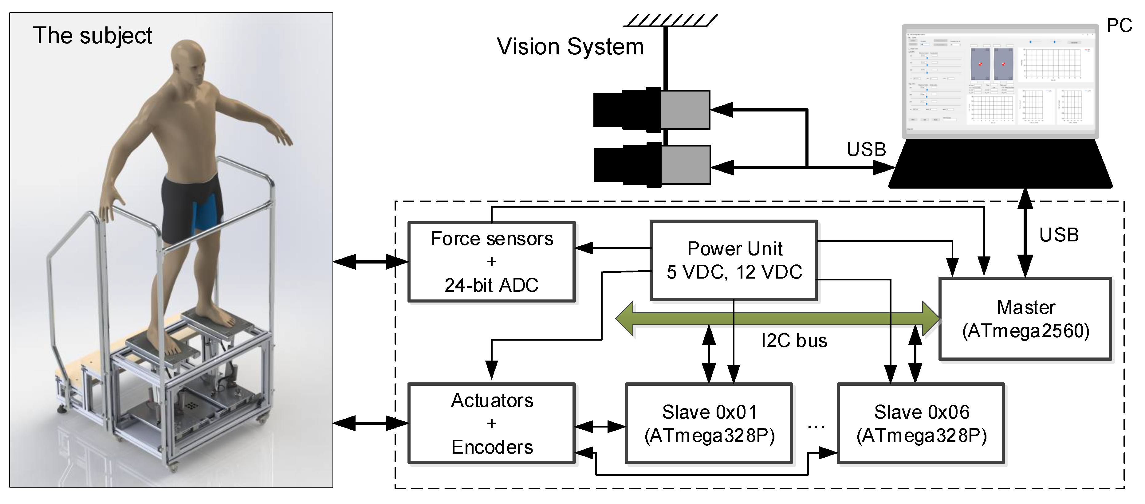
Figure 4.
System for evaluation and compensation of leg ength discrepancy for human body balancing.
Figure 4.
System for evaluation and compensation of leg ength discrepancy for human body balancing.
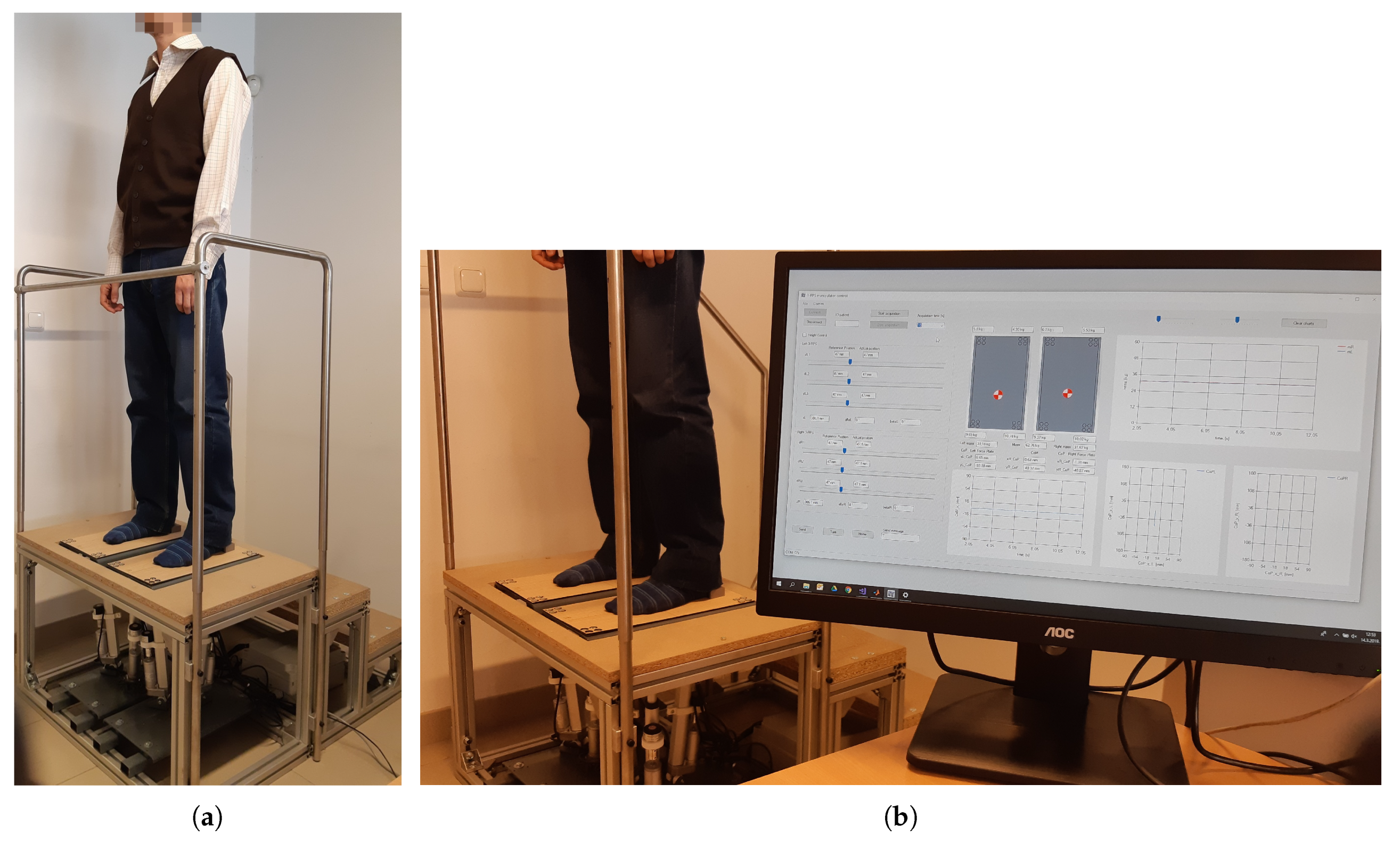
Figure 5.
Display of the mechanical set with two 3-RPS parallel manipulators with moving force plates: (a) with the patient on the force plates; and (b) with the application used to diagnose the load on each of the patient’s legs.
Figure 5.
Display of the mechanical set with two 3-RPS parallel manipulators with moving force plates: (a) with the patient on the force plates; and (b) with the application used to diagnose the load on each of the patient’s legs.
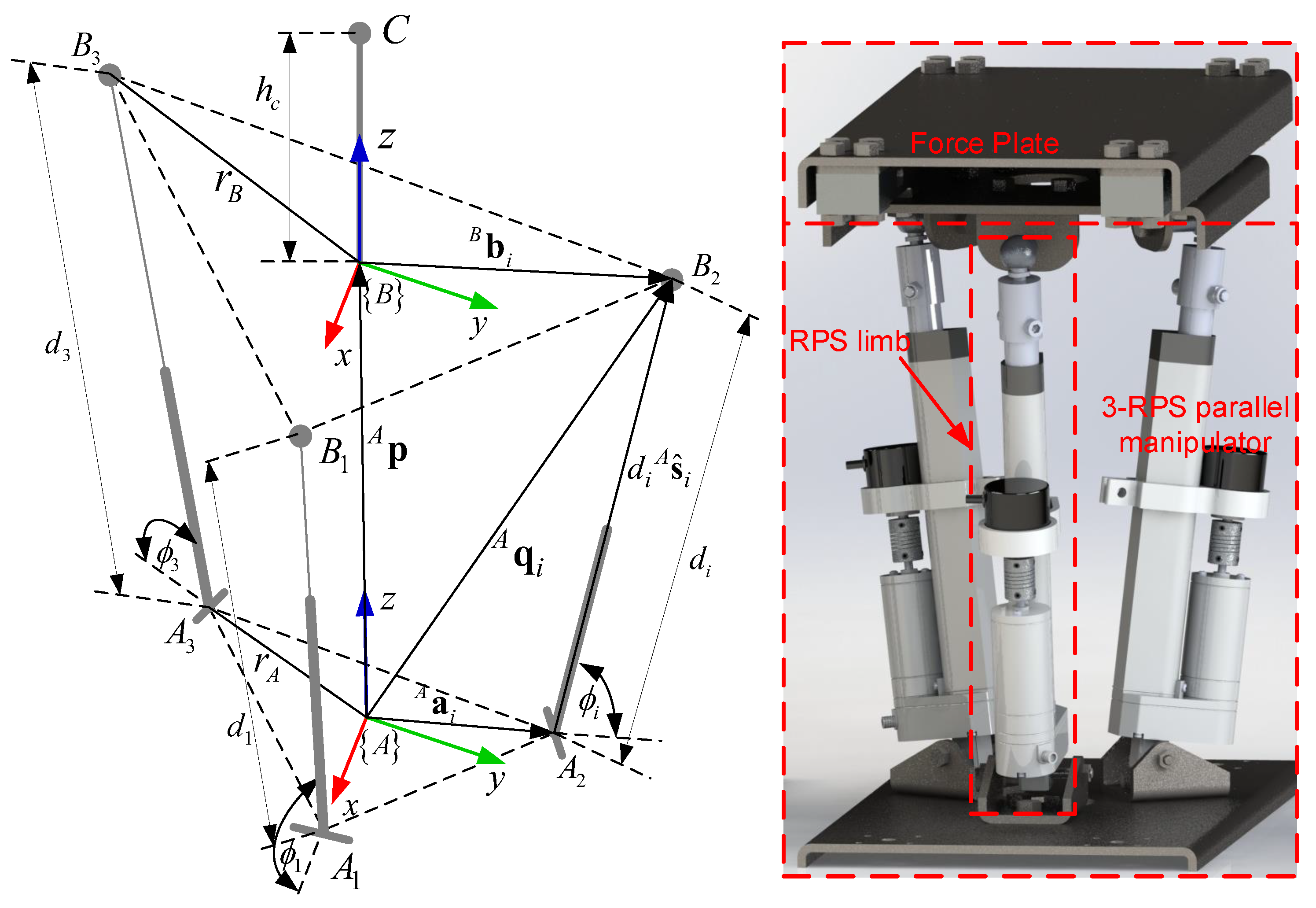
Figure 6.
Geometry of 3-RPS parallel manipulator.
Figure 6.
Geometry of 3-RPS parallel manipulator.
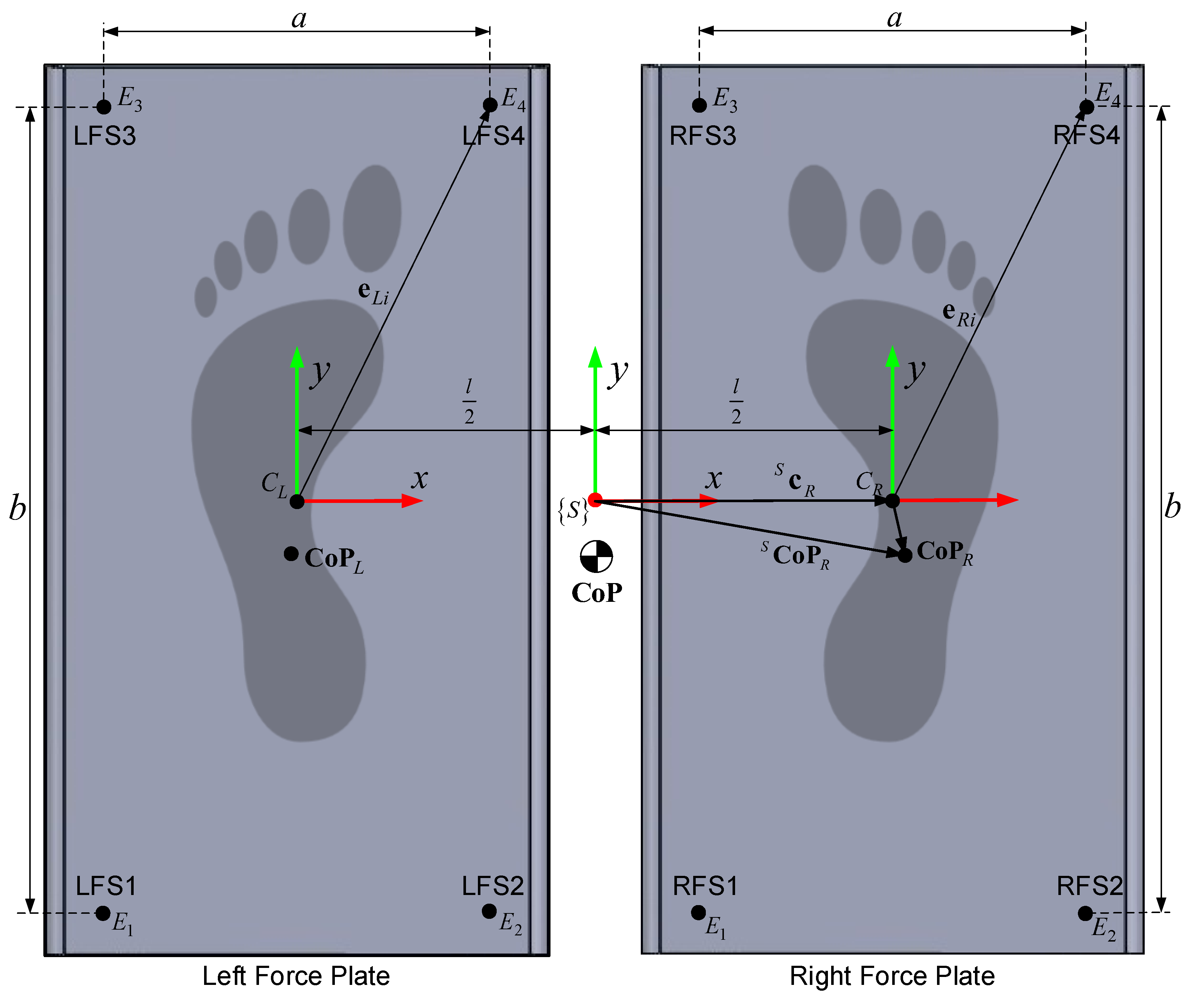
Figure 7.
Left and right leg force plate frames.
Figure 7.
Left and right leg force plate frames.
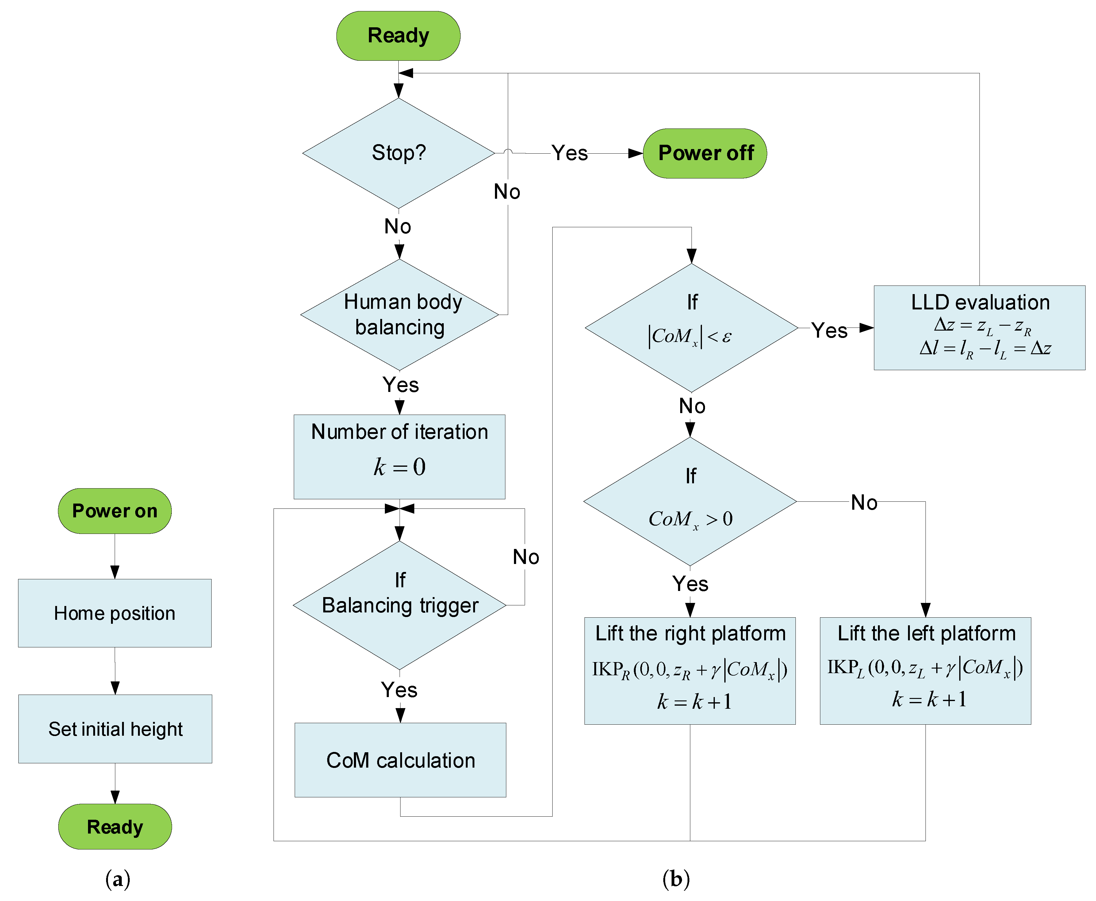
Figure 8.
Flowchart: (a) Turning the system on and moving the 3-RPS parallel manipulators to their initial height; and (b) Human Body Balancing Algorithm.
Figure 8.
Flowchart: (a) Turning the system on and moving the 3-RPS parallel manipulators to their initial height; and (b) Human Body Balancing Algorithm.
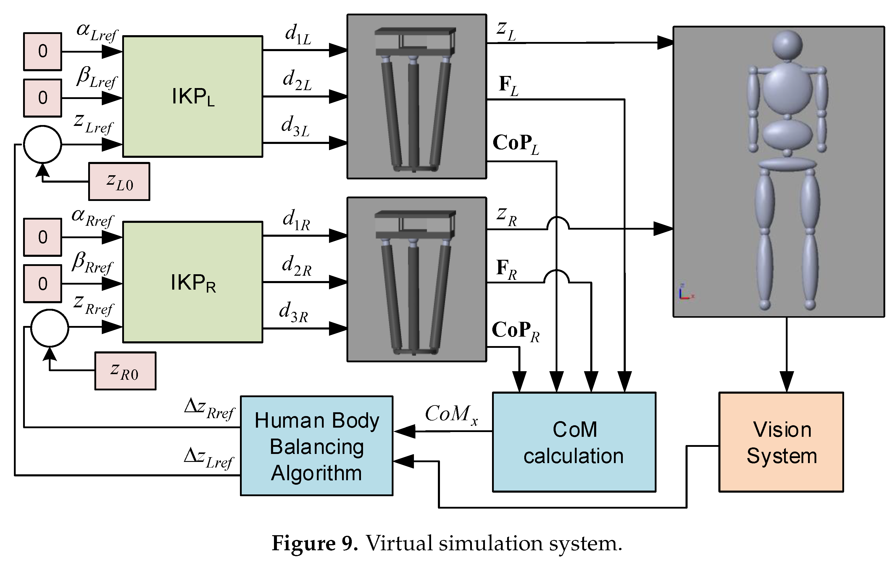
Figure 9.
Virtual simulation system.
Figure 9.
Virtual simulation system.
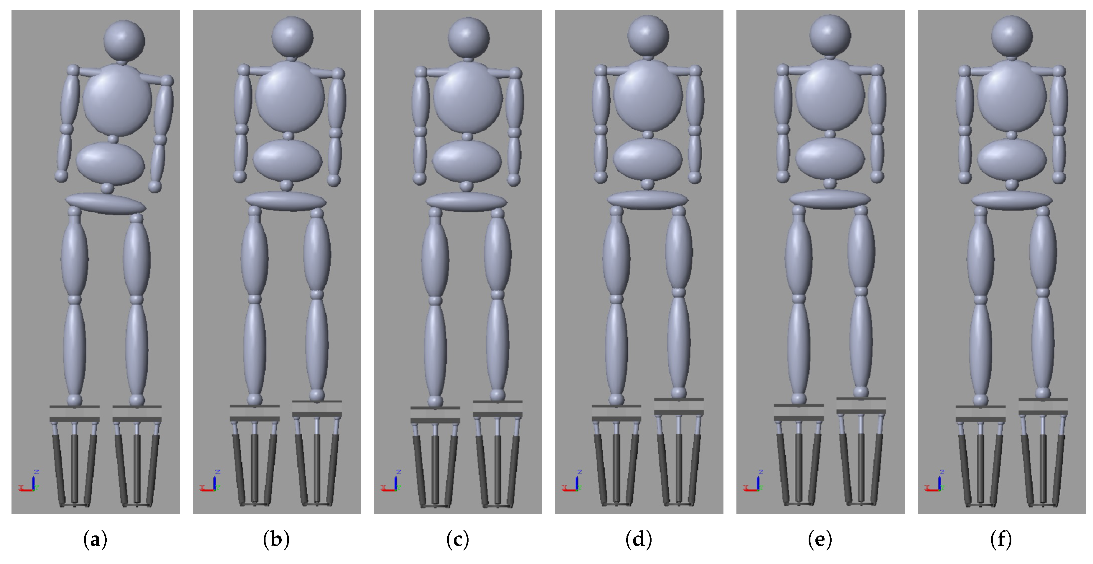
Figure 10.
Scenario 1: (a) Initial state of the human body with LLD (algorithm iteration k = 0); (b) algorithm iteration k = 1; (c) algorithm iteration k = 2; (d) algorithm iteration k = 3; (e) algorithm iteration k = 4; and (f) the human body is balanced (algorithm iteration k = 5).
Figure 10.
Scenario 1: (a) Initial state of the human body with LLD (algorithm iteration k = 0); (b) algorithm iteration k = 1; (c) algorithm iteration k = 2; (d) algorithm iteration k = 3; (e) algorithm iteration k = 4; and (f) the human body is balanced (algorithm iteration k = 5).
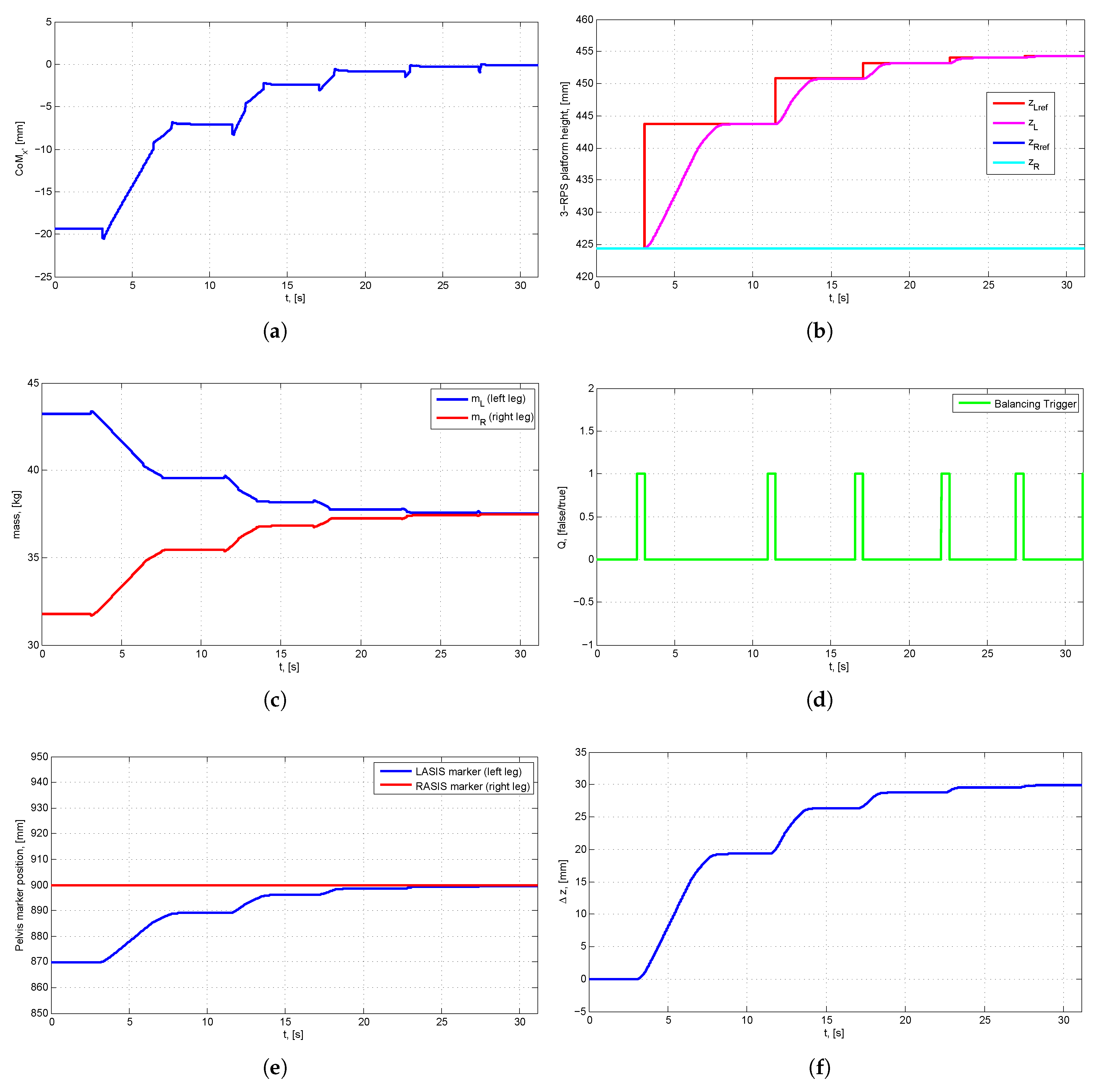
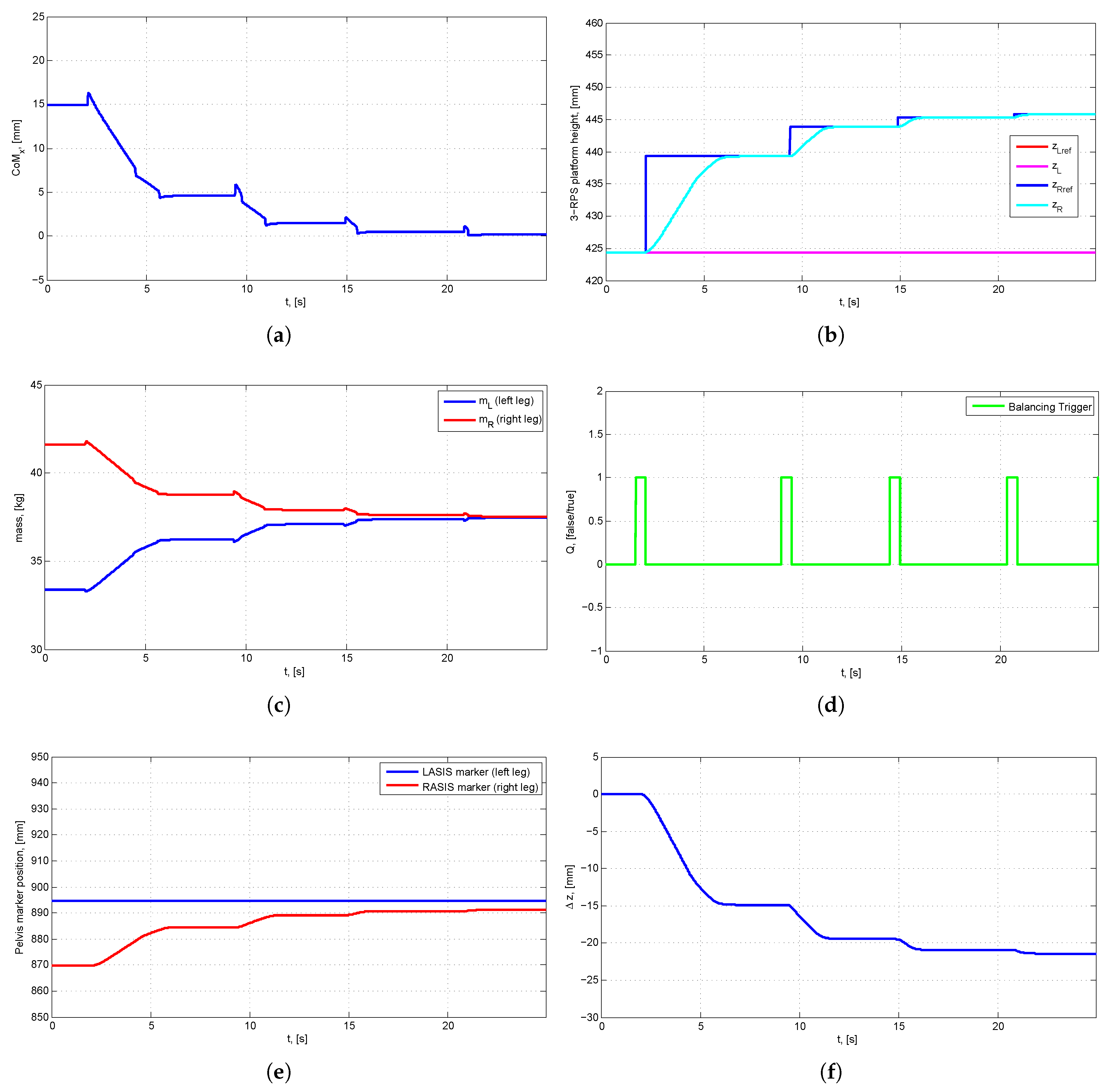
Figure 11.
Scenario 1: (a) , the position of the human body’s CoM; (b) reference height of the left () and right () force plate, current height of the left () and right () force plate; (c) the load on the left () and right () leg; (d) the balancing trigger signal (Q) marking the start of a new HBBA iteration; (e) position of the LASIS and RASIS markers, which are located on the pelvis; and (f) left and right force plate height difference (), which corresponds with the LLD evaluation () in the HBBA’s final step.
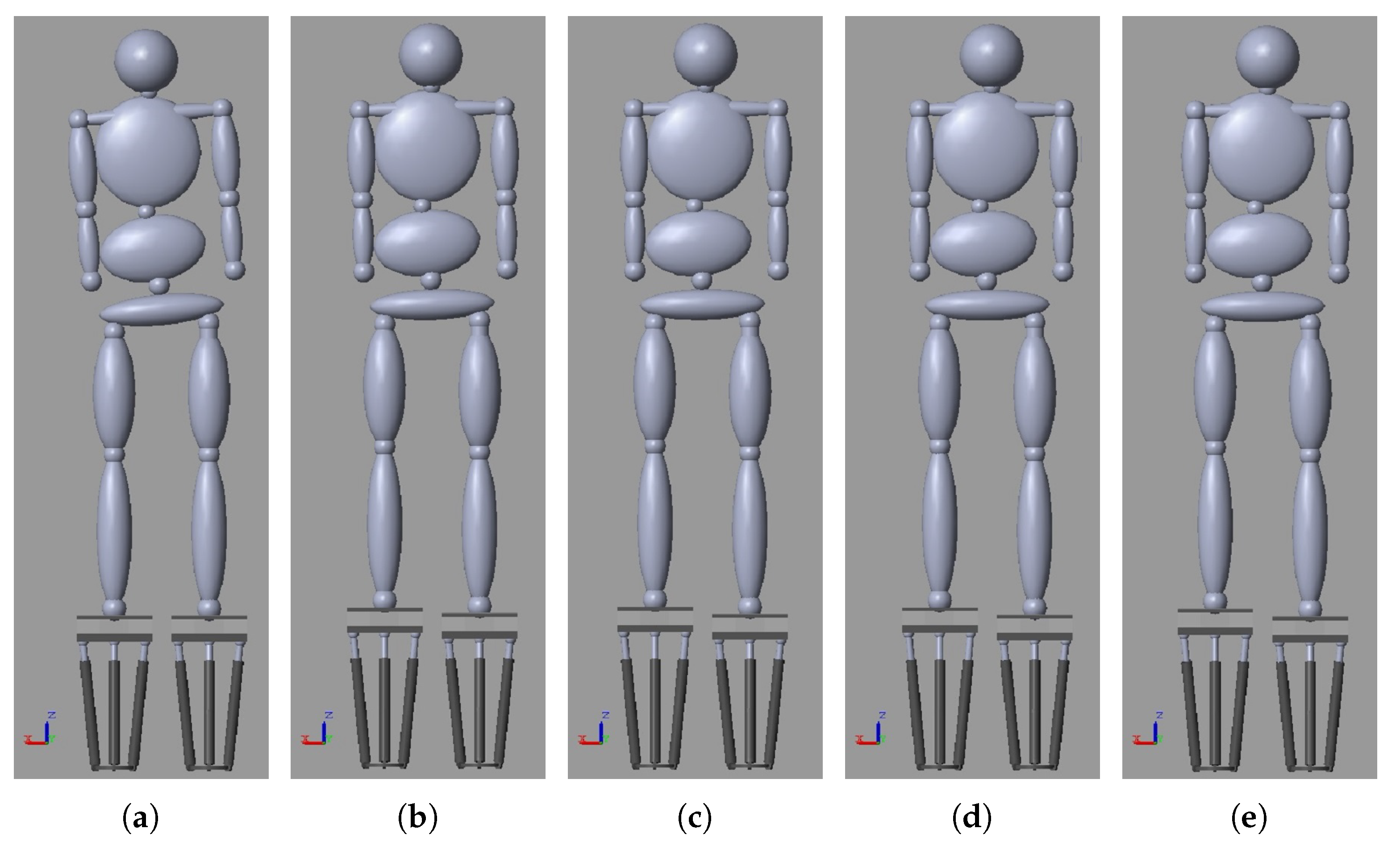
Figure 12.
Scenario 2: (a) Initial state of the human body with LLD and scoliosis (algorithm iteration k = 0); (b) algorithm iteration k = 1; (c) algorithm iteration k = 2; (d) algorithm iteration k = 3; and (e) the human body with LLD and scoliosis is balanced (algorithm iteration k = 4).
Figure 12.
Scenario 2: (a) Initial state of the human body with LLD and scoliosis (algorithm iteration k = 0); (b) algorithm iteration k = 1; (c) algorithm iteration k = 2; (d) algorithm iteration k = 3; and (e) the human body with LLD and scoliosis is balanced (algorithm iteration k = 4).
Figure 13.
Scenario 2: (a) , the position of the human body’s CoM; (b) reference height of the left () and right () force plate, current height of the left () and right () force plate; (c) the load on the left () and right () leg; (d) the balancing trigger signal (Q) marking the start of a new HBBA iteration; (e) position of the LASIS and RASIS markers, which are located on the pelvis; and (f) left and right force plate height difference (), which corresponds with the LLD evaluation () in the HBBA’s final step.
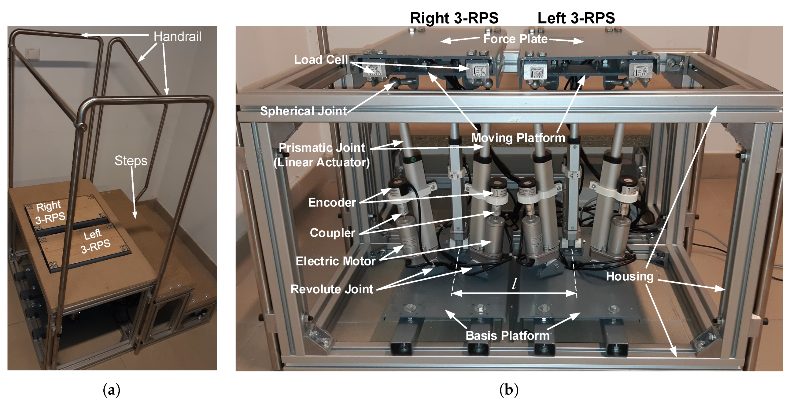
Figure 14.
Parts of the mechanical set with two 3-RPS parallel manipulators with moving force plates: (a) handrail and steps of the mechanical set; and (b) left and right 3-RPS parallel manipulators with moving force plates.
Figure 14.
Parts of the mechanical set with two 3-RPS parallel manipulators with moving force plates: (a) handrail and steps of the mechanical set; and (b) left and right 3-RPS parallel manipulators with moving force plates.
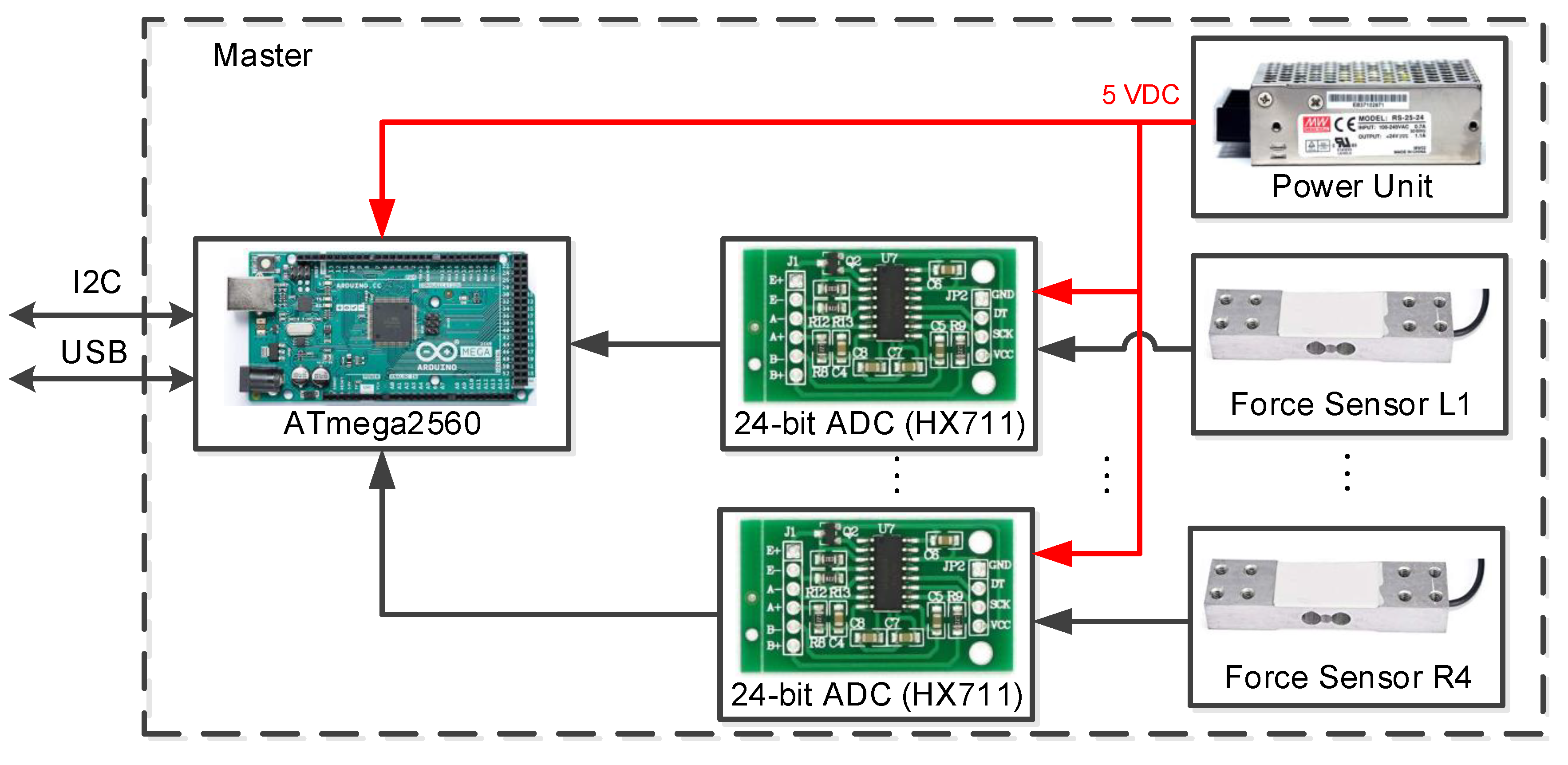
Figure 15.
Electronic schematic of the master device.
Figure 15.
Electronic schematic of the master device.
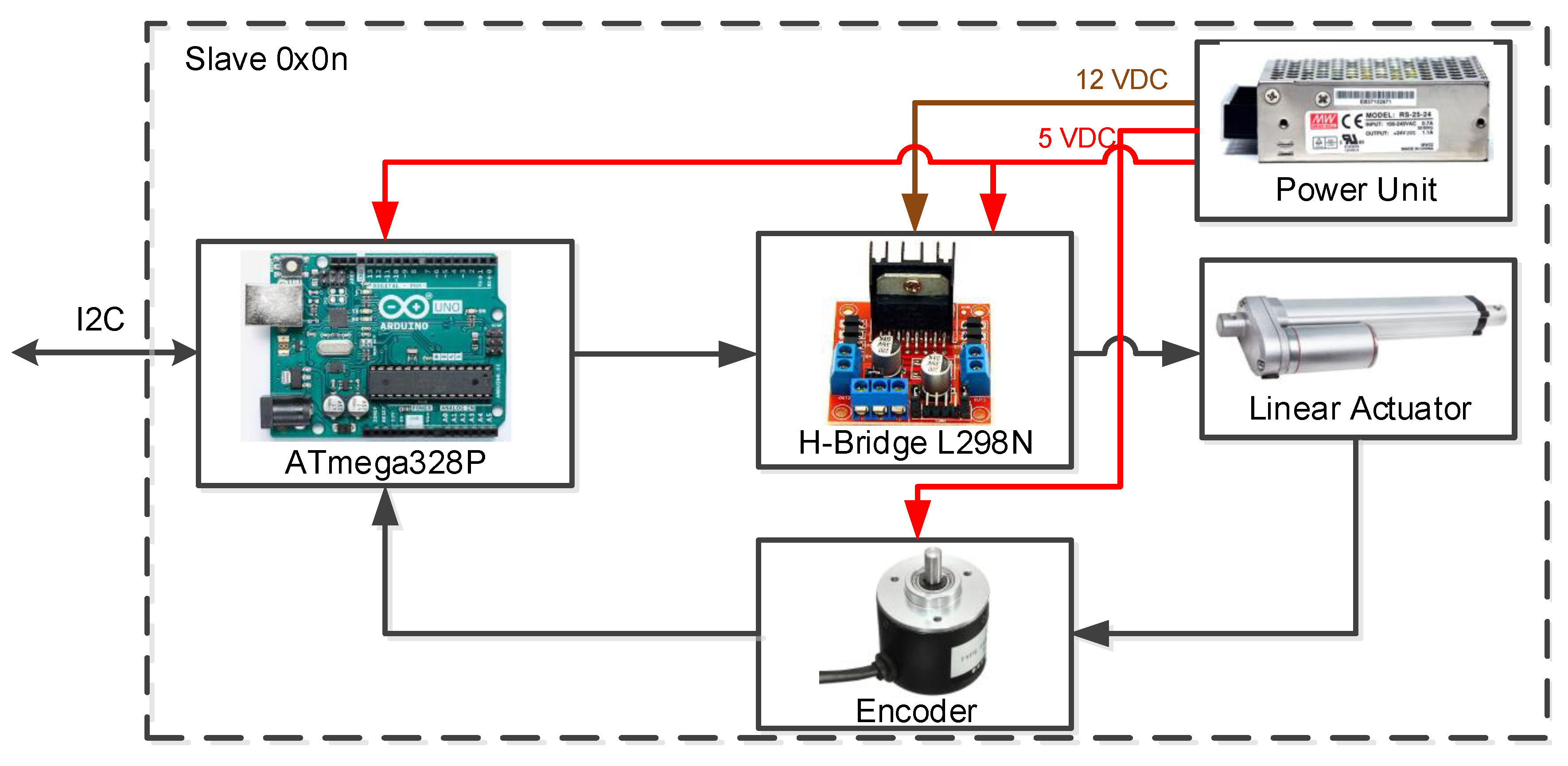
Figure 16.
Electronic schematic of the slave device.
Figure 16.
Electronic schematic of the slave device.
Figure 17.
PC application for control and data collection.
Figure 17.
PC application for control and data collection.
Figure 18.
Measurements of loads on the left and right legs and the CoM along the x-axis () for three chosen volunteers: (a) Volunteer 1, the loads on the left and the right legs; (b) Volunteer 1, CoM along the x-axis (); (c) Volunteer 2, the loads on the left and the right legs; (d) Volunteer 2, CoM along the x-axis (); (e) Volunteer 3, the loads on the left and the right legs; and (f) Volunteer 3, CoM along the x-axis ().
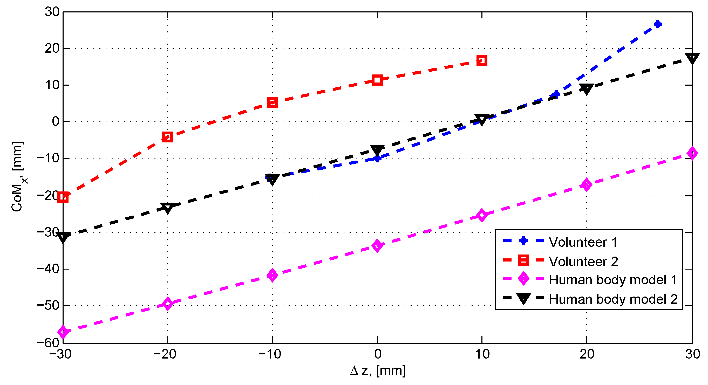
Figure 19.
Experiment 2: Shift of the CoM along the x-axis () depending on a force plate height difference .
Figure 19.
Experiment 2: Shift of the CoM along the x-axis () depending on a force plate height difference .
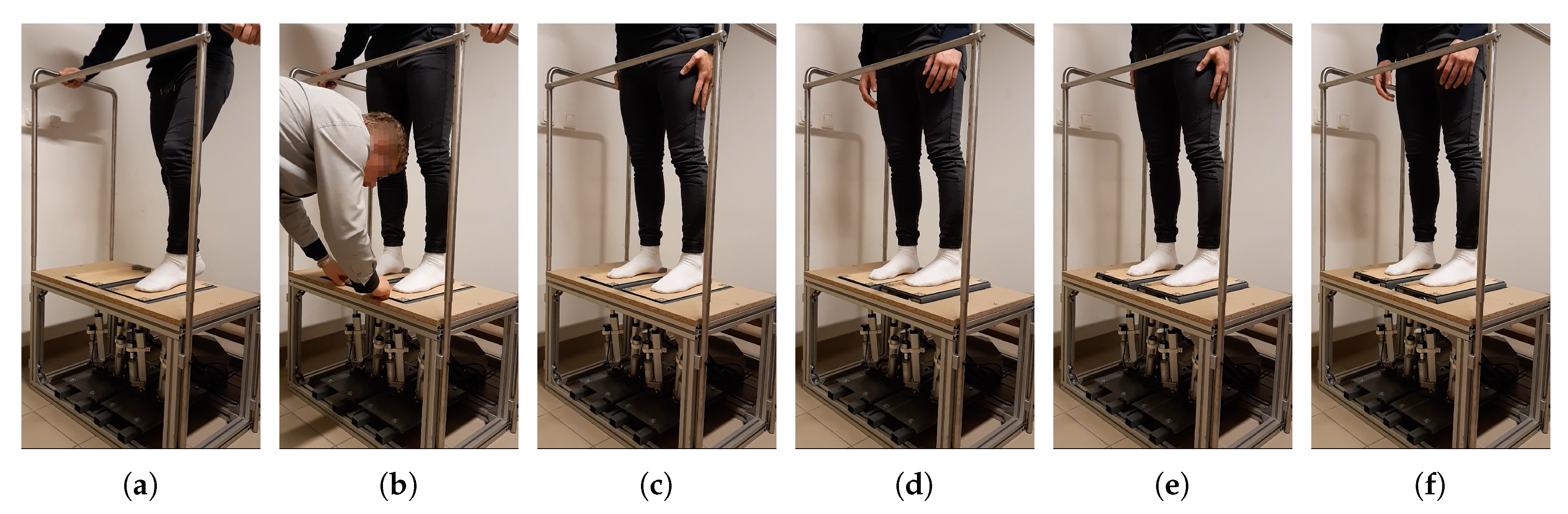
Figure 20.
Experiment 3: (a) Volunteer 3 placing the left leg on the force plate; (b) a researcher helps Volunteer 3 set the left and right legs on their respective marked locations; (c) Volunteer 3 is balanced (d) LLD simulation by shortening the right (lengthening the left) leg by 15 mm (initial algorithm state k = 0); (e) algorithm iteration k = 1; and (f) Volunteer 3 is balanced (algorithm iteration k = 2).
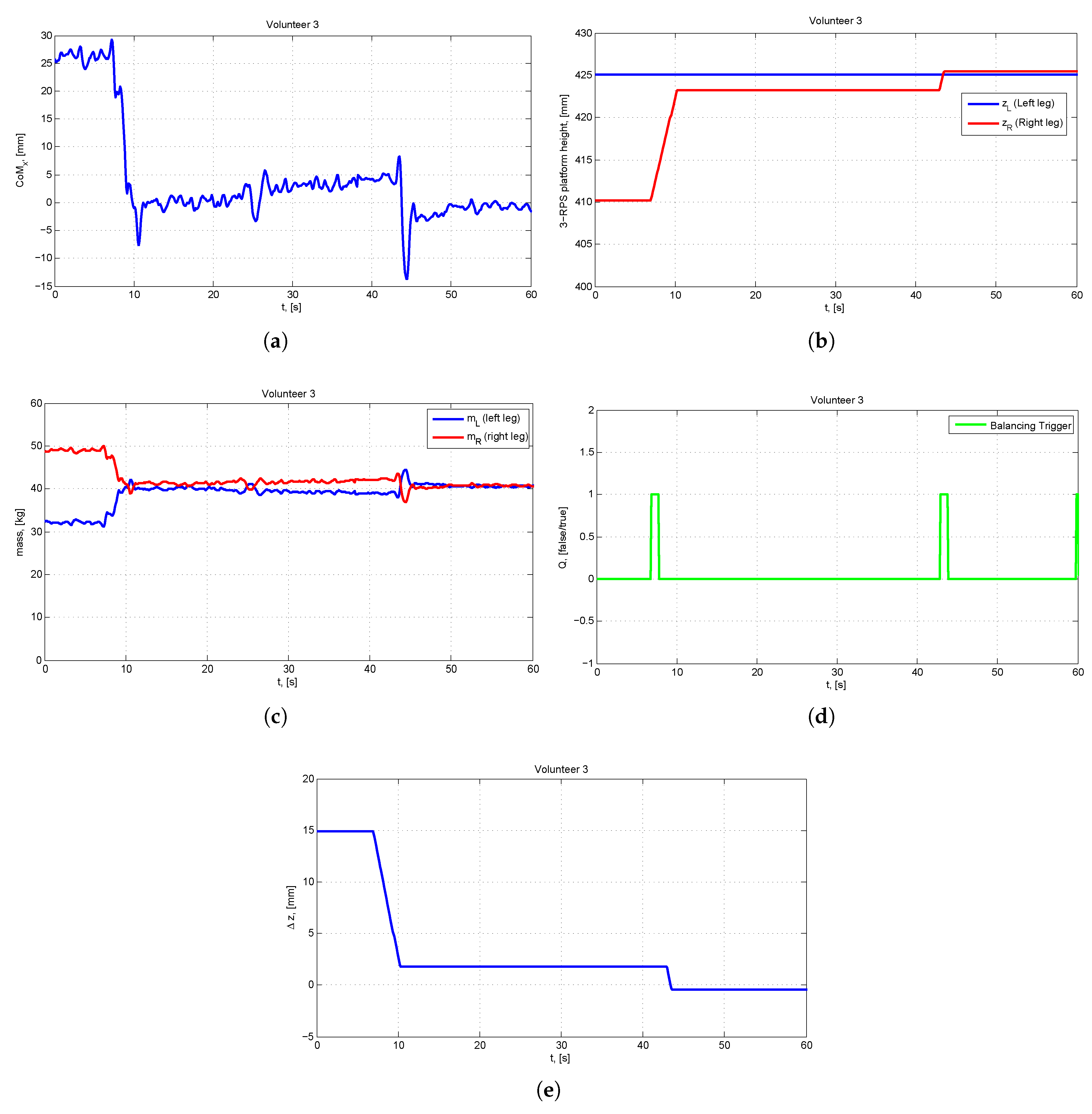
Figure 21.
Experiment 3: (a) , the position of the human body’s CoM; (b) reference height of the left () and right () force plate, current height of the left () and right () force plate; (c) the load on the left () and right () leg; (d) the balancing trigger signal (Q) marking the start of a new HBBA iteration; and (e) left and right force plate height difference (), which corresponds with the LLD evaluation () in the HBBA’s final step.
Table 1.
Scenario 1:
Figure 11 response values at the end each iteration of the HBBA.
Table 1.
Scenario 1:
Figure 11 response values at the end each iteration of the HBBA.
| Iteration | [mm] | [mm] | [mm] | [mm] | [kg] | [kg] | LASIS [mm] | RASIS [mm] |
|---|
| k = 0 | −19.35 | 424.40 | 424.40 | 0 | 43.22 | 31.78 | 869.8 | 899.8 |
| k = 1 | −7.06 | 443.75 | 424.40 | 19.35 | 39.53 | 35.47 | 889.1 | 899.8 |
| k = 2 | −2.42 | 450.81 | 424.40 | 26.41 | 38.19 | 36.81 | 896.1 | 899.8 |
| k = 3 | −0.81 | 453.23 | 424.40 | 28.83 | 37.73 | 37.27 | 898.5 | 899.8 |
| k = 4 | −0.27 | 454.04 | 424.40 | 29.64 | 37.58 | 37.42 | 899.4 | 899.8 |
| k = 5 | −0.09 | 454.31 | 424.40 | 29.91 | 37.53 | 37.47 | 899.7 | 899.8 |
Table 2.
Scenario 2:
Figure 13 response values at the end of each iteration of the HBBA.
Table 2.
Scenario 2:
Figure 13 response values at the end of each iteration of the HBBA.
| Iteration | [mm] | [mm] | [mm] | [mm] | [kg] | [kg] | LASIS [mm] | RASIS [mm] |
|---|
| k = 0 | 14.88 | 424.40 | 424.40 | 0 | 33.39 | 41.61 | 894.8 | 869.8 |
| k = 1 | 4.60 | 424.40 | 439.28 | −14.88 | 36.22 | 38.78 | 894.8 | 884.6 |
| k = 2 | 1.48 | 424.40 | 443.88 | −19.48 | 37.09 | 37.91 | 894.8 | 889.2 |
| k = 3 | 0.47 | 424.40 | 445.36 | −20.96 | 37.37 | 37.63 | 894.8 | 890.7 |
| k = 4 | 0.17 | 424.40 | 445.83 | −21.43 | 37.46 | 37.54 | 894.8 | 891.2 |
Table 3.
Experiment 1: Measurement results of the CoM along the x-axis (), mass, loads on the left () and right () legs, the positions of the LASIS and RASIS anatomical points, and the BMI. The loads on the left and right legs are shown as percentages [%] of the human body mass.
Table 3.
Experiment 1: Measurement results of the CoM along the x-axis (), mass, loads on the left () and right () legs, the positions of the LASIS and RASIS anatomical points, and the BMI. The loads on the left and right legs are shown as percentages [%] of the human body mass.
| Variable | | Mass [kg] | [%] | [%] | Height [cm] | LASIS [cm] | RASIS [cm] | BMI [kg m] |
|---|
| Mean | −2.99 | 75.26 | 51.12 | 48.88 | 174.9 | 101.2 | 101.2 | 24.45 |
| SD | 8.45 | 14.15 | 2.95 | 2.95 | 10.6 | 7.1 | 7.1 | 2.89 |
| Min | −27.08 | 53.68 | 44.90 | 41.94 | 155.0 | 88.0 | 88.0 | 18.72 |
| Max | 15.38 | 108.92 | 58.06 | 55.10 | 193.0 | 115.0 | 115.0 | 29.76 |
Table 4.
Measurement results of the CoM along the x-axis (), mass, loads on the left () and right () legs, the positions of the LASIS and RASIS anatomical points for three chosen volunteers.
Table 4.
Measurement results of the CoM along the x-axis (), mass, loads on the left () and right () legs, the positions of the LASIS and RASIS anatomical points for three chosen volunteers.
| Subject | | Mass [kg] | [kg] | [kg] | Height [cm] | LASIS [cm] | RASIS [cm] |
|---|
| Mean [mm] | SD [mm] |
|---|
| Volunteer 1 | 13.25 | 0.798 | 91.15 | 40.29 | 50.86 | 178 | 104 | 104 |
| Volunteer 2 | −9.80 | 0.490 | 55.34 | 29.44 | 25.90 | 157 | 96 | 96 |
| Volunteer 3 | −0.21 | 0.861 | 81.14 | 40.65 | 40.49 | 179 | 106 | 106 |
Table 5.
Experiment 3:
Figure 21 response values from for each iteration of the HBBA.
Table 5.
Experiment 3:
Figure 21 response values from for each iteration of the HBBA.
| Iteration | [mm] | [mm] | [mm] | [mm] | [kg] | [kg] |
|---|
| k = 0 | 26.4 | 425.0 | 410.0 | 15.0 | 32.16 | 48.98 |
| k = 1 | 4.4 | 425.0 | 423.2 | 1.8 | 39.21 | 41.94 |
| k = 2 | −0.6 | 425.0 | 425.4 | −0.4 | 40.73 | 40.46 |

 ,
, 


