Abstract
Previous studies have attempted to find autonomic differences of the cardiac system between the congestive heart failure (CHF) disease and healthy groups using a variety of algorithms of pattern recognition. By comparing previous literature, we have found that there are two shortcomings: (1) Previous studies have focused on improving the accuracy of models, but the number of features used has mostly exceeded 10, leading to poor generalization performance; (2) Previous works rarely distinguish the severity levels of CHF disease. In order to make up for these two shortcomings, we proposed two models: model A was used for distinguishing CHF patients from the normal people; model B was used for diagnosing the four severity levels of CHF disease. Based on long-term heart rate variability (HRV) (40000 intervals–8h) signals, we extracted linear and non-linear features from the inter-beat-interval (IBI) series. After that, the sequence forward selection algorithm (SFS) reduced the feature dimension. Finally, models with the best performance were selected through the leave-one-subject-out validation. For a total of 113 samples of the dataset, we applied the support vector machine classifier and five HRV features for CHF discrimination and obtained an accuracy of 97.35%. For a total of 41 samples of the dataset, we applied k-nearest-neighbor (K = 1) classifier and four HRV features for diagnosing four severity levels of CHF disease and got an accuracy of 87.80%. The contribution in this work was to use the fewer features to optimize our models by the leave-one-subject-out validation. The relatively good generalization performance of our models indicated their value in clinical application.
1. Introduction
Heart failure is the disability of the heart in pumping blood to the body efficiently [1]. Many previous works have confirmed that autonomic imbalance is the leading cause of congestive heart failure (CHF) disease. The autonomic nervous system (ANS) consists mainly of two branches, the sympathetic nervous system (SNS) and the parasympathetic nervous system (PNS) [2,3]. For the subjects in the normal group, the activities of two nervous systems are in a state of dynamic equilibrium. However, studies have shown that CHF breaks this equilibrium state due to excessive sympathetic activity [4]. The New York Heart Association (NYHA) has classified CHF into four scales based on the severity of the disease, NYHA I, II, III, and IV, respectively. Some papers have classified patients with mild heart failure (NYHA I or II) as low-risk patients and patients with severe heart failure (NYHA III or IV) as high-risk patients [5]. For patients with mild heart failure, the excessive activation of SNS and the continuous reduction of PNS activity would lead to an extreme imbalance of autonomic nerves if there is no suitable treatment, which would inevitably lead to further deterioration of the disease [5].
Heart rate variability (HRV), which represents the variation of inter-beat-interval, provides very useful information on the dynamics of heartbeat behavior [6,7]. Previous researchers have typically extracted linear and nonlinear HRV features from the inter-beat-interval (IBI) signals. The linear features are the signal parameters in time-domain, frequency-domain, and time-frequency domain [7,8,9]. In order to reveal other valuable information contained in the IBI signal, some researchers have used the complexity analysis method to extract nonlinear indicators [10,11,12,13,14,15,16,17,18,19,20]. In 2003, Asyali et al. [21] applied Bayesian classifiers and nine long-term measurements for CHF discrimination with an accuracy of 93.24%. In 2007, İşler et al. [22] utilized eight features of wavelet entropy and classical short-term HRV measurements and k-nearest-neighbor classifiers for CHF diagnosis and achieved an accuracy of 96.39%. In 2012, Yu et al. [23] applied support vector machine (SVM) classifier and genetic algorithm (GA) for CHF recognition and achieved an accuracy of 98.79%. In their work, 16 features by using bi-spectral heart rate (HR) analysis of short-term measurements were applied for CHF recognition [23]. In 2016, Acharya et al. [24] applied empirical mode decomposition (EMD) for automated identification of congestive heart failure. Using 22 short-term HRV measurements with support vector machines, they achieved an accuracy of 97.64% [24]. In 2017, Mahajan et al. [25] applied Ensemble classifiers and 10 short-term HRV measurements for CHF discrimination with an accuracy of 98.10%.
In 2013, Melillo et al. [5] tried to assess the severity levels of CHF disease by using long-term HRV measurements. The classification and regression tree (CART) classifier were used to separate lower-risk patients from higher-risk patients with an accuracy of 85.4%. In 2015, Shahbazi et al. [26] proposed a generalized discriminant analysis method, applied k-nearest-neighbor classifier for CHF risk assessment based on long-term HRV, and obtained an accuracy of 100%. In 2016, Chen et al. [27] built a four-level risk assessment model for CHF detection and quantification based on the DT-SVM (decision tree based support vector machine) algorithm. The model obtained a total accuracy of 96.61% in risk assessment among individuals of N (no risk), P1 (mild risk), P2 (moderate risk), and P3 (severe risk) [27]. In that paper, they used 180 features, including 126 dynamic measurements and 54 static measurements [27]. In 2019, Li et al. [28] proposed a four-stage classification problem using an end to end deep model, which extracted 20 features by convolution at max-pooling layers, and an accuracy of 97.6% was achieved.
From the previous work above, we have found that there are two points which need to be further explored: 1) They have focused on improving the accuracy of models, but the number of features in their pattern recognition models mostly exceeds 10 [23,24,25,27,28]. However, the limited number of features improves certainly the interpretability of the classification; 2) Compared with the diagnosis of the severity levels of CHF, researchers were more inclined to diagnose CHF patients from normal people. For CHF risk assessment, their research was the consolidation of multiple NYHA scales into one category for identification [5,26,27,28]. Therefore, researchers rarely distinguished the four severity scales of CHF disease clearly, which is a four-class classification problem. In view of the above-mentioned reasons, we proposed two models based on long-term HRV (40,000 HRV intervals–8h): model A was used for distinguishing CHF patients from the normal people (binary classification); model B was used for diagnosing the four severity levels of CHF disease (four-class classification). Detailed processes of building the two models are described in the following sections.
2. Materials
2.1. Data Collection
In previous studies, the RR interval time series (RRITS) was often used as the data source for analyzing HRV measures [21,22,23,24,25,26,27]. The RRITS was calculated as the interval between two consecutive R peaks of heartbeat in the electrocardiographic (ECG) signals. The data we studied were all from the RRITS database in the PhysioBank server. The data can be downloaded online from http://www.physionet.org/cgi-bin/atm/ATM for free. Each recording in the RRITS database was manually reviewed and corrected by experts. Supported by the National Research Resource Center of the National Institutes of Health, the PhysioBank server is a joint project involving many research and medical institutions [29,30].
As shown in Table 1, our study used a total of four RRITS databases. A total of 116 24-hour RR interval recordings were included in the dataset of 72 normal subjects and 44 CHF subjects. The data of normal subjects comes from two databases: the MIT/BIH Normal Sinus Rhythm Database (Nrsdb) and the Normal Sinus Rhythm RR Interval Database (Nrs2db) [29]. The data of CHF patients were obtained from the BIDMC Congestive Heart Failure Database (Chfdb) and the Congestive Heart Failure RR Interval Database (Chf2db) [30]. Due to the lack of recordings of NYHA IV CHF patients in the CHF RR database, we labeled NYHA III-IV CHF patients as NYHA IV CHF patients in the database.

Table 1.
RR interval time series (RRITS) database with the normal and congestive heart failure (CHF) subjects.
2.2. Data Preprocessing
The flowchart of the data processing is given in Figure 1. We first downloaded the RRITS signal from the public database. However, we found that RRITS included too many ectopic heartbeat intervals that cover up important physiological information [5]. According to beat annotations files provided from the database, we removed the ectopic intervals of each RRITS signal with manual review and correction. Therefore, the NN interval time series will be obtained by removing all ectopic intervals, such as ventricular ectopic, supraventricular ectopic, or unknown. In order to ensure the reliability of the signal, the ratio of the length of the NN interval time series to the length of the RRITS (NN/RR) was calculated. The ratio was used as a measure of data reliability to exclude the recordings where the ratio was less than the threshold. In general, the ratio is set to 80% because it is a satisfactory compromise between the number of subjects included in the research work and the NN signal quality [5]. Based on the above excluding criterion, one recording was excluded from each of NYHA II, NYHA III, and NYHA IV CHF groups, respectively. Finally, we randomly selected continuous 40,000 NN intervals as one segment for each recording. As shown in Table 2, we obtained 113 samples for building model A, including 72 healthy samples and 44 CHF samples. We obtained 41 samples for building model B, including 4 NYHA I CHF samples, 7 NYHA II CHF samples, 16 NYHA III CHF samples, and 14 NYHA IV CHF samples.
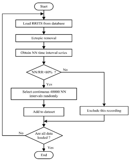
Figure 1.
Flowchart of the data processing in this study. RRITS: RR interval time series.
Table 2.
Dataset for building model A and B.
It was necessary to specify that in order to make the HRV signals more stable and homogeneous when extracting the frequency domain features, some previous researchers removed the linear trend of the HRV signal and used the cubic-spline interpolation method to re-sample it at a rate of 4 samples per second [22,23,31,32]. However, we applied the Lomb-Scargle (LS) periodogram proposed in [31,32] to calculate the power spectrum. In this case, HRV signals did not require resampling in our research [33,34].
3. Methods
After preprocessing the HRV signals, we extracted linear and nonlinear features. Then, the sequence forward selection (SFS) algorithm was used to reduce the dimension of the feature space. Finally, a variety of classification algorithms were used for building model A and B, and the models with the best performance were selected.
3.1. Feature Extraction
3.1.1. Linear Feature
Features extracted in the time-domain and frequency-domain are listed in Table 3 [7,8]. We extracted 8 time-domain features in this study. Frequency-domain HRV measures were analyzed based on the estimation of the power spectrum (PSD) through the LS method. After estimating PSD, three main spectral components were distinguished from the spectrum: very low frequency (VLF), low frequency (LF), and high frequency (HF) components. These frequency bands were bounded with the limits 0–0.04, 0.04–0.15, and 0.15–0.40 Hz, respectively [7]. To a certain extent, frequency-domain HRV measures reflected the activity of the autonomic system. As described in Table 3, we extracted 8 frequency-domain HRV features.
Table 3.
Heart rate variability (HRV) measures in the time-domain and frequency-domain.
In addition to the classical HRV measures, we also used time-frequency domain measures based on the wavelet theory. HRV signal fluctuates in an irregular and complex manner [35]. Quantification power of the features based on time-domain and frequency-domain analysis is limited when analyzing non-stationary HRV signals. Therefore, we characterized and quantified the non-stationary properties of physiological signals based on wavelet theory. We used the mother wavelet ‘db4’ to perform a 4-scale decomposition. From the low frequency to high frequency, we got 5 frequency bands, and the wavelet coefficients of 5 bands were CA4, CD4, CD3, CD2, and CD1, respectively. Then, the mean and the standard deviation of the coefficients of each band were calculated [9,36]. Finally, we extracted 10 features based on the time-frequency domain.
3.1.2. Non-Linear HRV Features
In this paper, non-linear indicators were obtained by local Hurst exponent analysis based on the wavelet theory, detrended fluctuation analysis (DFA), entropy analysis, and Poincare plot analysis.
Biomedical signals are generated by complex self-regulating systems that process inputs with a wide range of characteristics [10,11]. Previous studies have shown that HRV signals with healthy people are a multi-fractal signal. However, the HRV signal with CHF patients is approximately a single fractal signal [10,11]. The fractal properties are characterized by Δh (Δh = hmax − hmin, h is the Hurst exponent) [11]. In 1999, Ivanov et al. [11] evaluated the local Hurst exponent h through the modulus of the maxima values of the wavelet transform at each point in the time series and scales a = 2 × 1.15i, i = 10,...41. They have found the Hurst exponent has a great ability to distinguish CHF patients from normal people [11]. We analyzed the fractal characteristics of the subjects based on long-term HRV signals. The scales in our research were consistent with other papers, i.e., a = 2 × 1.15i, i = 10,...41.
DFA is often used to quantify HRV signals. This technique is a modification of root-mean-square analysis of random walks applied to non-stationary signals [12,13]. In this paper, we extracted two features using the DFA algorithm: α1 was obtained by least square fitting of F(n) and small scale n (4 ≤ n ≤ 16); α2 was obtained by least square fitting of F(n) and larger scale n than 16.
Sample entropy (SampEn) and fuzzy measure entropy (FuzzyMEn) are often used as measures for the analysis of the complexity of HRV signals [14,15,16,17]. Usually, SampEn and FuzzyMEn are influenced by the parameters of embedding dimension m and tolerance threshold r [16,17]. In this paper, the best combination of m and r for SampEn and FuzzyMEn were obtained by statistical significance analysis.
The Poincare plot can reflect the nonlinear characteristics of the nature of the HRV signal. It is a graph of each RR (or NN) interval against the next interval [18,19]. In this article, we extracted three features based on the Poincare diagram analysis, i.e., SD1 (the width of the Poincare plot), SD2 (the length of the Poincare plot), and SD1/SD2 [20].
3.2. Feature Selection
We extracted 34 features, including 26 linear features and 8 non-linear features in our research. For high-dimension feature sets, building models directly has a large computation cost [37]. On the contrary, the limited number of features improves certainly the interpretability of the classification [37]. Therefore, it is necessary to use the feature selection method to find the best feature subset. This optimal feature subset uses the least number of features to get the best performance of the classifier [37]. In this paper, we used the SFS algorithm for reducing the feature dimension. SFS algorithm is a bottom-up search procedure, which starts from an empty feature set and adds one feature at each iteration step by using some evaluation functions [38,39]. In this paper, we used the classification performance of the classifier as the evaluation function of the feature selection process.
3.3. Classification
In order to build models with the best performance, our work applied a variety of classification algorithms, including support vector machine (SVM), linear discriminant analysis (LDA), k-nearest-neighbor (KNN), decision tree (DT), and Bayesian (NB). Relevant principles of classification algorithms can be referred to the previous studies [21,22,23,24,25,26,27]. The kernel function for SVM classifier was a radial basis function. We used the five algorithms mentioned for building model A and B. All features were normalized between 0 and 1 using the min-max method proposed in [22,32] before classification.
The performance of different classifiers was evaluated by the indicators of precision (Prec), sensitivity (Sens), specificity (Spec). The calculation of these three evaluation indicators refers to Equations (1)–(3). Besides, AUC, i.e., the area under the ROC (receiver operating characteristic) curve, was also simply calculated by Equation (4) [5,40]. To compute these estimators, true positives (TP), true negatives (TN), false positives (FP), and false negatives (FN) should be measured first. For the four-class classification, we divided the problem into four 2-class classifications. In each 2-class problem, we viewed one kind of NYHA scales as a positive case and the other three NYHA scale as negative cases.
After building the models, there are usually two ways to validate the performance of the models:
Cross-subject validation [36,41]: If the dataset has N subjects, and one subject provides n samples, this validation uses all the samples (m × n samples for the test set) from m different subjects as the test set, and uses all the remaining samples ((N−m) × n samples for training set) to train the classifier. This way one can obtain M accuracies by training M models if the m subjects selected each time are different from each other. Then, the average of M accuracies as the final accuracy of models is calculated.
Intra-subject validation [36,41]: The common ten-fold cross-validation is this way. Because this method of validation requires random scrambling of samples, it will result in multiple samples for each subject being present in both the test set and the training set.
Obviously, compared with cross-subject validation, the intra-subject validation usually obtains a higher recognition rate [24,42]. However, the model using intra-subject validation does not predict well for unknown data. On the contrary, this shows that the models using cross-subject validation and obtaining accuracy have a great application value. Since each subject in our study provided a segment, the leave-one-subject-out was cross-subject validation for evaluating models [22,23,32,40].
4. Results
4.1. The Setting of Feature Parameters
- The nonlinear feature α1 was extracted based on the DFA algorithm, and the small scale n ranges were from four to 16. Different ranges of the large scale n () show very different quantification power for HRV signals. In order to find an optimal scale range for large scale n, we analyzed the statistical difference of the feature α2 between the normal and CHF groups. The span of the scale range is 48, and the length of the sliding step is four.
As shown in Table 4 and Figure 2, α2 was significantly different between the normal and CHF groups at the n values of 16 ≤ n ≤ 64, 56 ≤ n ≤ 104, 60 ≤ n ≤ 108, with 16 ≤ n ≤ 64 corresponding to the smallest p-value (p = 4 × 10⁻⁴ by Student’s t-test, marked red in Figure 2). Therefore, we chose 16 ≤ n ≤ 64 for the calculation of feature α2.
Table 4.
The statistical t-test results of the feature α2 in the 14 scale ranges for the normal and congestive heart failure (CHF) groups.
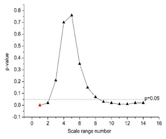
Figure 2.
The quantification power (p-value) of the feature α2.
Table 5 gives the statistical F-test results of the feature α2 with various scales for CHF disease with four severity levels. The F-test is generally used for the significant test between multiple groups. According to the statistical results, the feature α2 was not statistically significantly different in all scales for CHF diseases with different severity levels. The range of scale from 16 to 64 was relatively better than other ranges and was applied for calculating feature α2 when building model B.
Table 5.
The statistical F-test results of the feature α2 in the 14 scale ranges for four severity levels of congestive heart failure (CHF).
- 2.
- Different parameters (m and r) of sample entropy (SampEn) and fuzzy measure entropy (FuzzyMEn) also lead to different quantification power of HRV signals. In order to find the best combinations of parameters, the parameter m changed from one to three with a step of one, and r changed from 0.10 to 0.20 with a step of 0.05. For the normal and CHF groups, Table 6 gives the statistical Kolmogorov-Smirnov (KS) test results of SampEn and FuzzyMEn with a different combination of parameters. For CHF diseases with different severity levels, Table 7 gives the statistical F-test results of SampEn and FuzzyMEn with different combinations of parameters.
Table 6. The statistical Kolmogorov-Smirnov (KS) test results of the sample entropy (SampEn) and fuzzy measure entropy (FuzzyMEn) with different combinations of m and r for the normal and congestive heart failure (CHF) groups.
Table 7. The statistical F-test results of the sample entropy (SampEn) and fuzzy measure entropy (FuzzyMEn) with different combinations of m and r for the different severity levels of congestive heart failure (CHF).
As shown in Table 6, m = 1 and r = 0.15 obtained the SampEn values with the most significant statistical difference (p = 1 × 10⁻³ by KS test) between the two groups; m = 1 and r = 0.20 got the FuzzyMEn values with the most significant statistical difference (p = 9 × 10⁻⁷ by KS test) between the two groups. Therefore, m = 1 and r = 0.15 was set for SampEn, and m = 1 and r = 0.20 for FuzzyMEn in model A. Similarly, based on F-test results in Table 7, m = 1 and r = 0.10 was set for SampEn and FuzzyMEn in model B.
4.2. Validation
4.2.1. Model A
Table 8 shows the leave-one-subject-out validation performance of model A for different classification algorithms. The highest accuracy of 97.35% was achieved by using both SVM and KNN (K = 1) classifiers. However, the SVM used fewer features (number of features (NF) = 5) to achieve the same accuracy of KNN (K = 1). In order to better apply model A to the clinical diagnosis of CHF disease, we tried our best to make CHF patients not misdiagnosed as normal subjects. Therefore, with the same accuracies of SVM and KNN (K = 1), the sensitivity indicator was an important index. For the sensitivity and AUC indicators, the performance of the SVM was (Sensitivity = 97.56% and AUC = 0.963) better than the performance of KNN (K = 1, Sensitivity = 95.12%, and AUC = 0.959). Therefore, considering the better NF, sensitivity, accuracy, and AUC, our work used the SVM classifier to build model A.
Table 8.
Performance parameters of various classifier algorithms for building model A.
4.2.2. Model B
After accurately diagnosing CHF disease, it was necessary to categorize the four severity levels of the CHF disease. Considering that NYHA I CHF patients only have four recordings, the value of K cannot be too large for KNN algorithm. In our research, the value of K equaled 1, 3, and 5, respectively. Table 9 briefly shows the leave-one-subject-out validation parameters of model B for each classification algorithm. We applied KNN (K = 1) classifier and four features for building model B with the highest accuracy of 87.80%. The selected best features were seen to be PNN20, PNN50, TOTPWR, and FuzzyMEn, respectively. In order to further analyze the performance of the model, we divided the four-class classification problem into four binary classification problems. In each binary classification problem, one severity level of CHF disease was considered to be the target class, and other severity levels of CHF disease were considered to be the negative class. Table 10 shows the leave-one-subject-out validation performance of the KNN (K=1) classifier for building model B. For mild CHF disease (CHF I-II), the values of precision and sensitivity are smaller than those of severe CHF disease (CHF III-IV). The reason is that the number of mild CHF subjects is too small.
Table 9.
The performance parameters of five classifier algorithms for building model B.
Table 10.
Performance of the k-nearest-neighbor (KNN) (K = 1) classifier for building model B.
5. Discussion
5.1. Comparison of Similar Work
Table 11 highlights the results in previous related studies that used HRV signals as the data source for analysis. The accuracy of models built by previous researchers has exceeded 95%, which indicated that there is a big difference in the cardiac system between the normal and CHF groups. However, the number of features they used mostly exceed 10. In contrast, we applied the SVM classifier and only five features for model A with an accuracy of 97.35%. We used a larger sample size to build our model A to make it more stable than previous studies. Previous work is more inclined to find the difference between the normal and CHF groups. In Table 11, researchers have evaluated the different severity levels of CHF disease, and a large number of features were used for binary and four-class classifications [27,28].
Table 11.
Comparison between related previous work and our work.
However, we applied the KNN (K = 1) classifier and four features for diagnosing the four severity levels of CHF disease with an accuracy of 87.80%. In 2016, Acharya et al. [24] divided the RRITS of each recording in the database into a segment with 2000 intervals and applied the SVM classifier and 22 features for CHF discrimination with an accuracy of 97.60%. In 2018, Li et al. [42] divided the RRITS of each recording in the database into a segment with 300 intervals and applied the CNN classifier and one feature for CHF discrimination with an accuracy of 81.85%. In these two papers, one subject provided more than one RRITS segments in the database, and the use of ten-fold cross-validation to evaluate the performance of classifier means that the data of the training set and the data of the test set may come from the same subject. That was to say, the evaluation of these two models was intra-subject and not cross-subject validation. Because of large similarities between multiple segments of the same subject, intra-subject validation of evaluating models tended to achieve an over-optimistic accuracy. However, the two models we built were evaluated using more robust cross-subject validation, and a higher accuracy was obtained.
5.2. Limitations of This Study
We used 113 subjects to build the two proposed models. As we can see from Table 1 and Table 2, the number of NYHA I and NYHA II CHF subjects was significantly smaller than that of NYHA III and NYHA IV CHF subjects. For the lack of recordings of NYHA IV CHF patient in the CHF RR database, we labeled NYHA III-IV CHF patients as NYHA IV CHF patients in the database. Obviously, the small number and imbalance of the dataset will make it difficult to further improve the accuracies of the classifiers [44,45]. Besides, due to the relatively small amount of recordings, we only leave one subject for cross-validation. As long as our dataset is small and unbalanced, it is impossible to confirm the generalization of our results unless a larger public dataset is available [44,45]. Therefore, we still need to validate our models with larger dataset in the future.
6. Conclusions
This paper proposed two models for automatic CHF diagnosis. Model A was used for distinguishing CHF patients from normal people (binary classification), and model B was used to diagnosing four severity levels of CHF diseases (four-class classification). Model A applied the SVM classifier and five HRV indicators (TOTPWR, PLF/PHF, SD1, α2, and SampEn) with an accuracy of 97.35%. Model B applied the KNN (K = 1) classifier and four HRV indicators (PNN20, PNN50, TOTPWR, and FuzzyMEn) with an accuracy of 87.80%. The advantage of model A and B was the use of a small amount of features while ensuring that the model has high accuracy. This advantage indicated the application value of our models in clinical practice.
Author Contributions
Conceptualization, Z.H. and W.W.; Methodology, Z.H.; Validation, Z.H. and W.W.; Formal analysis, C.C. and R.Z.; Data curation, C.C. and R.Z.; Writing—original draft preparation, Z.H.; writing—Review and editing, G.L. and W.W.
Funding
This research was funded by the National Science Foundation of China (Grant No. 61103132 and No. 61872301) and the Fundamental Research Funds for the Central Universities of China (Grant No. XDJK2013A020).
Acknowledgments
The authors would like to thank all the participants taken part in the experiments.
Conflicts of Interest
The authors declare no conflict of interest.
References
- Flavell, C.; Stevenson, L.W. Take heart with heart failure. Circulation 2001, 104, 89–91. [Google Scholar] [CrossRef][Green Version]
- Floras, J.S. Sympathetic nervous system activation in human heart failure: clinical implications of an updated model. J. Am. Coll. Cardiol. 2009, 54, 375–385. [Google Scholar] [CrossRef] [PubMed]
- Schwartz, P.J. Vagal stimulation for heart diseases: from animals to men. - An example of translational cardiology. Jpn. Circ. J. 2011, 75, 20–27. [Google Scholar] [CrossRef]
- Kishi, T. Heart failure as an autonomic nervous system dysfunction. J. Cardiol. 2012, 59, 117–122. [Google Scholar] [CrossRef] [PubMed]
- Melillo, P.; De, L.N.; Bracale, M.; Pecchia, L. Classification tree for risk assessment in patients suffering from congestive heart failure via long-term heart rate variability. IEEE J. Biomed. Health Inform. 2013, 17, 727–733. [Google Scholar] [CrossRef]
- Akselrod, S.; Gordon, D.; Madwed, J.B.; Snidman, N.C.; Shannon, D.C.; Cohen, R.J. Hemodynamic regulation: investigation by spectral analysis. Am. J. Physiol. 1985, 249, 867–875. [Google Scholar] [CrossRef] [PubMed]
- Malik, M.; Bigger, J.T.; Camm, A.J.; Kleiger, R.E.; Malliani, A.; Moss, A.J.; Schwartz, P.J. Heart rate variability Standards of measurement, physiological interpretation, and clinical use. Ann. Noninvas. Electrocardiol. 1996, 93, 1043–1065. [Google Scholar] [CrossRef]
- Montano, N.; Ruscone, T.G.; Porta, A.; Lombardi, F.; Pagani, M.; Malliani, A. Power spectrum analysis of heart rate variability to assess the changes in sympathovagal balance during graded orthostatic tilt. Circulation 1994, 90, 1826–1831. [Google Scholar] [CrossRef]
- Yang, F.; Liao, W. Modeling and decomposition of HRV signals with wavelet transforms. IEEE Eng. Med. Biol. Mag. 1997, 16, 17–22. [Google Scholar] [CrossRef]
- Ivanov, P.C.; Zhi, C.; Hu, K.; Stanley, H.E. Multiscale aspects of cardiac control. Physica A 2004, 344, 685–704. [Google Scholar] [CrossRef][Green Version]
- Ivanov, P.C.; Amaral, L.A.; Goldberger, A.L.; Havlin, S.; Rosenblum, M.G.; Struzik, Z.R.; Stanley, H.E. Multifractality in human heartbeat dynamics. Nature 1999, 399, 461–465. [Google Scholar] [CrossRef]
- Peng, C.K.; Havlin, S.; Hausdorff, J.M.; Mietus, J.E.; Stanley, H.E.; Goldberger, A.L. Fractal mechanisms and heart rate dynamics *: Long-range correlations and their breakdown with disease. J. Electrocardiol. 1995, 28, 59. [Google Scholar] [CrossRef]
- Huikuri, H.V.; Makikallio, T.H.; Peng, C.; Goldberger, A.L.; Hintze, U.; Moller, M. Fractal Correlation Properties of R-R Interval Dynamics and Mortality in Patients with Depressed Left Ventricular Function After an Acute Myocardial Infarction. Circulation 2000, 101, 47–53. [Google Scholar] [CrossRef]
- Lake, D.E.; Richman, J.S.; Griffin, M.P.; Moorman, J.R. Sample entropy analysis of neonatal heart rate variability. Am J. Physiol. Regul. Integr. Comp. Physiol. 2002, 283, R789. [Google Scholar] [CrossRef]
- Liu, C.; Zhao, L. Using Fuzzy Measure Entropy to improve the stability of traditional entropy measures. In Proceedings of the Computing in Cardiology, Hangzhou, China, 18–21 September 2011; pp. 681–684. [Google Scholar]
- Zhao, L.; Wei, S.; Zhang, C.; Zhang, Y.; Liu, C. Determination of Sample Entropy and Fuzzy Measure Entropy Parameters for Distinguishing Congestive Heart Failure from Normal Sinus Rhythm Subjects. Entropy 2015, 17, 6270–6288. [Google Scholar] [CrossRef]
- Wang, Y.; Wei, S.; Zhang, S.; Zhang, Y.; Zhao, L.; Liu, C.; Murray, A. Comparison of time-domain, frequency-domain and non-linear analysis for distinguishing congestive heart failure patients from normal sinus rhythm subjects. Biomed. Signal Process. Control 2018, 42, 30–36. [Google Scholar] [CrossRef]
- Rn, M.A.W.; Stevenson, W.G.; Moser, D.K.; Trelease, R.B.; Harper, R.M. Patterns of beat-to-beat heart rate variability in advanced heart failure. Am. Heart J. 1992, 123, 704. [Google Scholar]
- Marciano, F.; Migaux, M.L.; Acanfora, D.; Furgi, G.; Rengo, F. Quantification of Poincare’ maps for the evaluation of heart rate variability. In Proceedings of the Computers in Cardiology, Bethesda, MD, USA, 25–28 September 1994; pp. 577–580. [Google Scholar]
- Brennan, M.; Palaniswami, M.; Kamen, P. Do existing measures of Poincaré plot geometry reflect nonlinear features of heart rate variability? IEEE Trans. Biomed. Eng. 2001, 48, 1342–1347. [Google Scholar] [CrossRef]
- Asyali, M.H. Discrimination power of long-term heart rate variability measures. In Proceedings of the International Conference of the IEEE Engineering in Medicine and Biology Society, Cancun, Mexico, 17–21 September 2003; pp. 200–203. [Google Scholar]
- İşler, Y.; Kuntalp, M. Combining classical HRV indices with wavelet entropy measures improves to performance in diagnosing congestive heart failure. Comput. Biol. Med. 2007, 37, 1502–1510. [Google Scholar] [CrossRef]
- Yu, S.N.; Lee, M.Y. Bispectral analysis and genetic algorithm for congestive heart failure recognition based on heart rate variability. Comput. Biol. Med. 2012, 42, 816–825. [Google Scholar] [CrossRef]
- Acharya, U.R.; Fujita, H.; Sudarshan, V.K.; Oh, S.L.; Muhammad, A.; Koh, J.E.W.; Tan, J.H.; Chua, C.K.; Chua, K.P.; Tan, R.S. Application of empirical mode decomposition (EMD) for automated identification of congestive heart failure using heart rate signals. Neural Comput. Appl. 2017, 28, 3073–3094. [Google Scholar] [CrossRef]
- Mahajan, R.; Viangteeravat, T.; Akbilgic, O. Improved detection of congestive heart failure via probabilistic symbolic pattern recognition and heart rate variability metrics. Int. J. Med. Inform. 2017, 108, 55–63. [Google Scholar] [CrossRef]
- Shahbazi, F.; Asl, B.M. Generalized discriminant analysis for congestive heart failure risk assessment based on long-term heart rate variability. Comput. Methods Programs Biomed. 2015, 122, 191–198. [Google Scholar] [CrossRef]
- Chen, W.; Zheng, L.; Li, K.; Wang, Q.; Liu, G.; Jiang, Q. A Novel and Effective Method for Congestive Heart Failure Detection and Quantification Using Dynamic Heart Rate Variability Measurement. PLoS ONE 2016, 11, e0165304. [Google Scholar] [CrossRef]
- Li, D.; Li, X.; Zhao, J.; Bai, X. Automatic staging model of heart failure based on deep learning. Biomed. Signal Process. Control 2019, 52, 77–83. [Google Scholar] [CrossRef]
- Goldberger, A.L.; Amaral, L.A.N.; Glass, L.; Hausdorff, J.M.; Ivanov, P.C.; Mark, R.G.; Mietus, J.E.; Moody, G.B.; Peng, C.; Stanley, H.E. PhysioBank, PhysioToolkit, and PhysioNet Components of a New Research Resource for Complex Physiologic Signals. Circulation 2000, 101, 215–220. [Google Scholar] [CrossRef] [PubMed]
- Facc, D.S.B.; Facc, W.S.C.; Monrad, E.S.; Smith, H.S.; Wright, R.F.; Lanoue, A.; Gauthier, D.F.; Ransil, B.J.; Grossman, W.; Braunwald, E. Survival of patients with severe congestive heart failure treated with oral milrinone. J. Am. Coll. Cardiol. 1986, 7, 661–670. [Google Scholar]
- Tarvainen, M.P.; Rantaaho, P.O.; Karjalainen, P.A. An advanced detrending method with application to HRV analysis. IEEE Trans. Biomed. Eng. 2002, 49, 172–175. [Google Scholar] [CrossRef]
- Narin, A.; Isler, Y.; Ozer, M. Investigating the performance improvement of HRV Indices in CHF using feature selection methods based on backward elimination and statistical significance. Comput. Biol. Med. 2014, 45, 72–79. [Google Scholar] [CrossRef] [PubMed]
- Laguna, P.; Moody, G.B.; Mark, R.G. Power spectral density of unevenly sampled data by least-square analysis: performance and application to heart rate signals. IEEE Trans. Biomed. Eng. 1998, 45, 698–715. [Google Scholar] [CrossRef]
- Clifford, G.D.; Lionel, T. Quantifying errors in spectral estimates of HRV due to beat replacement and resampling. IEEE Trans. Biomed. Eng. 2005, 52, 630–638. [Google Scholar] [CrossRef] [PubMed]
- Stanley, H.E.; Ahlers, G. Introduction to Phase Transitions and Critical Phenomena. Phys. Today 1973, 26, 71–72. [Google Scholar] [CrossRef]
- Chen, L.; Zhao, Y.; Ye, P.; Zhang, J.; Zou, J. Detecting driving stress in physiological signals based on multimodal feature analysis and kernel classifiers. Expert Syst. Appl. 2017, 85, 279–291. [Google Scholar] [CrossRef]
- Biagetti, G.; Crippa, P.; Falaschetti, L.; Orcioni, S.; Turchetti, C. Multivariate Direction Scoring for Dimensionality Reduction in Classification Problems. In Intelligent Decision Technologies; Czarnowski, I., Caballero, A., Howlett, R., Jain, L., Eds.; Springer: Cham, Switzerland, 2016. [Google Scholar]
- Kudo, M.; Somol, P.; Pudil, P.; Shimbo, M.; Sklansky, J. Comparison of Classifier-Specific Feature Selection Algorithms. In Advances in Pattern Recognition; Ferri, F.J., Iñesta, J.M., Amin, A., Pudil, P., Eds.; Lecture Notes in Computer Science; Springer: Berlin/Heidelberg, Germany, 2000; Volume 1876, pp. 677–686. [Google Scholar]
- Schenk, J.; Kaiser, M.; Rigoll, G. Selecting Features in On-Line Handwritten Whiteboard Note Recognition: SFS or SFFS? In Proceedings of the International Conference on Document Analysis and Recognition, Barcelona, Spain, 26–29 July 2009; pp. 1251–1254. [Google Scholar]
- Pecchia, L.; Melillo, P.; Sansone, M.; Bracale, M. Discrimination Power of Short-Term Heart Rate Variability Measures for CHF Assessment. IEEE Trans. Inform. Technol. Biomed. 2011, 15, 40–46. [Google Scholar] [CrossRef] [PubMed]
- Li, X.; Song, D.; Zhang, P.; Zhang, Y.; Hou, Y.; Hu, B. Exploring EEG Features in Cross-Subject Emotion Recognition. Front. Neurosci. 2018, 12, 162. [Google Scholar] [CrossRef]
- Li, Y.; Zhang, Y.; Zhao, L.; Zhang, Y.; Liu, C.; Zhang, L.; Zhang, L.; Li, Z.; Wang, B.; Ng, E.Y.K. Combining Convolutional Neural Network and Distance Distribution Matrix for Identification of Congestive Heart Failure. IEEE Access 2018, 6, 39734–39744. [Google Scholar] [CrossRef]
- Guidi, G.; Pettenati, M.C.; Melillo, P.; Iadanza, E. A Machine Learning System to Improve Heart Failure Patient Assistance. IEEE J. Biomed. Health Inform. 2014, 18, 1750–1756. [Google Scholar] [CrossRef]
- Ali, A.; Shamsuddin, S.M.; Ralescu, A.L. Classification with class imbalance problem: a review. Int. J. Adv. Soft Comput. Appl. 2013, 5, 176–204. [Google Scholar]
- Zou, Q.; Xie, S.; Lin, Z.; Wu, M.; Ju, Y. Finding the Best Classification Threshold in Imbalanced Classification. Big Data Res. 2016, 5, 2–8. [Google Scholar] [CrossRef]


© 2019 by the authors. Licensee MDPI, Basel, Switzerland. This article is an open access article distributed under the terms and conditions of the Creative Commons Attribution (CC BY) license (http://creativecommons.org/licenses/by/4.0/).