Abstract
This article analyses the dispersion of vibration accelerations of a railway bridge during the passage of a train, and presents an analysis of their parameters after the application of the theory of covariance functions. The measurements of vibration accelerations at the fixed points of the beams of the overlay of the bridge were recorded in the time scale as digital arrays (matrices). The values of inter-covariance functions of the arrays of data of measurements of digital vibration accelerations and the values of auto-covariance functions of the individual arrays, changing the quantization interval in the time scale, were calculated. The compiled software Matlab 7 in the operator package environment was used in calculations. This article aims at determining the interdependencies of results of vibrations of bridge points rather than at the impact which a train makes on a bridge without emphasizing the modal parameters of the bridge. The aforementioned interdependencies make it possible to predict the results of hard-to-reach points.
1. Introduction
An analysis of the dispersion of vibration accelerations of the beams of the railway bridge overlay with a locomotive moving at 60 km/h and a freight train moving at 80 km/h was conducted in this study [1]. The theory of covariance functions was used in the analysis of vibration parameters. Graphical expressions of covariance functions illustrate the change of inter-dependence of vibration parameters over a given time scale [2]. The degree of the change of spatial dependences depends on technological and dynamic properties of the object being examined and the stability of the structure of the bridge trusses [3].
Many articles have been written on analyses of rail bridge vibrations. Such research has mainly focused on bridge conditions [4], such as a resonance mechanism explained by Xia et al. [5], vibration mode-coupling and intermittent contact loss and vibration instability in a large motion bistable compliant mechanism by Nikman et al. [6,7], the stability of dynamic response by Capsoni et al. [8], the dependence of bridge vibration parameters on cross winds by Xu et al. [9] and the use of bridge-track-vehicle element by Cheng et al. [10].
There are methods described in literature (1, 2 and 3 [11,12,13]) aimed at optimizing the number of metering points. Although there may be many different algorithms for the placement of sensors in order to optimize the number and locations of sensors on the structure, increasing the volume of available information is the key criterion identified in the examined sources of literature [14,15]. The purpose of the information received is to identify structural defects or to provide information on structural changes (usually using modal analysis). Artificial Neural Networks (ANNs), Pattern Search (PS) and Evolutionary Strategies (ES), such as the Genetic Algorithms (GA) [5], the Particle Swarm Optimization (PSO) [6], and the Covariance-Matrix Adaptation Evolution Strategy (CMA-ES) are some of the countless examples available in the literature [7,16,17,18]. This article focuses on analysing hard-to-reach significant points (because the examined object is an old-structure bridge that is not adapted for dynamic research) by performing dynamic load tests (with a train moving at different speeds). This article is aimed at determining the interdependencies of results of vibrations of bridge points rather than the impact that a train makes on a bridge without emphasizing the modal parameters of the bridge. The identification of the aforementioned interdependencies makes it possible to predict the results of hard-to-reach points.
Methods of reversal analysis efficiently support studies of vibrations of railway bridges. Simplification of the measurement process and fewer sensors for determining vibration parameters make it possible to use the received compositional models. Diagnosing bridge condition status with the proposed methods is an important bridge resource forecasting tool for assessing the moving level of moving rolling stocks. The aim of this paper is to show that the proposed method can be used to assess the dependence of accelerometer points, and thus, that fewer sensors can be used in the experiment (because of a complicated bridge design, it is often impossible to physically measure significant acceleration of bridge points because of a difficult access to the bridge).
There are many ways to diagnose bridge structures. The assessment of bridge structures is very important because of long service life, structural deformations, natural wear and tear and increasing need for axle load. A dynamic enhancement factor (DAF), which determines dynamic impact of moving trains on the bridge, is an important factor. The accurate assessment of DAF ensures sustainable management of existing bridges [1]. Assessing the main natural frequencies and mode forms of the bridge is of particular importance [19]. They can also be monitored using GAMMA Portable Radar Interferometer (GPRI) [20]. The TTB model could also be used for testing rail bridge parameters, and shows that shorter wavelengths are important for safety analyses. Longer wavelengths are more relevant to vehicle train quality [21]. It is also possible to apply the linear superposition principle to analyses of the fatigue characteristics of rail bridges [22]. The bridge model can be supplemented with mechanical bridge performance tests and approved using the FEM bridge model [23].
2. Modelling Vibration Parameters
Accelerometers were placed on beams and the vibrations of the beams were measured. Sensors were positioned on the upper plane (i.e., the top view). The sensor layout was selected to display dynamic variations at all significant points. Signals received during measurements were processed using Brüel & Kjær software (Sampling frequency 400 Hz). The weight of the moving locomotive was 119 t. The tests were conducted under the same environmental conditions, namely, the temperature was 30 °C and humidity was at 70%.
The array of vibration accelerations consists of 8 vectors. Data of vectors 1–4 capture accelerations of the rear steady point 1 of the railway bridge beam at time intervals during the movement of the locomotive (vectors 1 and 2) and train (vectors 3 and 4). Vectors 1 and 3 show changes in vertical acceleration, while vectors 2 and 4 show changes in longitudinal acceleration. The data of vectors 5–8 show the change of the vertical accelerations of the mid-points of beams 1 and 2 of the railway bridge at time intervals 0.00097 s during the movement of a locomotive (vectors 5 and 6) and a train (vectors 7 and 8) [11].
The study presents a means to calculate of the most reliable trend values of the vibration vector which uses the least squares method. The trend of the vibrations vector is assumed to be a discrete dimension with a fixed value. The use of the least squares method partially eliminates random vibration errors. When processing large-scale measurement data, the method of the least squares also provides asymptotically effective values of the calculated parameters when the distribution of the measurement data is not normal [12].
The array of the measurement of vibration accelerations consists of 8 vectors (columns). Each vector is understood as a random function with random measurement errors. In application of the method of least squares, the most reliable trend value, also called the weighted average, is calculated for each vector [13]. Assuming that the vector trend value differs according to the harmonic law, when the forecasted wave length corresponds to the length of the vibration acceleration vector, the parametric equation of a single vector value is expressed as:
where is the random acceleration error, is the acceleration value, and is the acceleration vector trend. Coefficient is expressed as:
where
is the value of the unit of measure, rad, Equation (1) in the expression of matrices is expressed as:
where is the vector of random errors, is the vector of vibrations accelerations, and is the matrix of coefficients of parametric equations [14].
The most reliable trend value of the vibration acceleration vector is calculated using the condition of the method of the least squares:
where is the diagonal matrix of weight of vibration accelerations.
Weights of single acceleration values are calculated according to the formula:
where is the standard deviation of the measurement result the weight of which is assumed to be equal to 1 . Thus, the value is chosen freely because it has no impact on the calculation results. The measurement result is selected for weights to be close to 1 (to reduce the scope of calculations).
From the equation
the following value is derived:
Formula (6) shows that the value of depends on the value of vibration acceleration . Thus, acceleration of a higher value is less accurate, because
Using formula (5) the following is obtained:
where the acceptable average value is
The extremity of the function (4) is determined by finding its partial derivatives according to the parameter , equating it to zero and having solved the equation [15]:
we receive:
and
The solution is equal to zero.
where
The accuracy of estimates of parameters calculated in application of the method of the least squares is assessed by their covariance matrix [15].
3. Object of the Research and Measurement Results
In this article, an old bridge in Jonava, Kaunas district, Republic of Lithuania, was chosen as the object of research. It was built in 1914 but destroyed during the World War II by the Soviet Union and Nazi German troops. A new railway bridge was built in 1948. The aim of this article was to evaluate the dynamic parameters of the railway bridge after more than 70 years of intensive operation.
Signals received during measurements were processed using Brüel & Kjær software (Figure 1) [15]. Signal filtering was used to eliminate noises in observance of the requirements laid down in source [17,18] which require considering frequencies to the greater of: (a) 30 Hz, (b) frequency of the main form of vibrations of the element being examined multiplied by 1.5; (c) frequency of the third form of vibrations of the element.
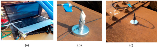
Figure 1.
Brüel & Kjær measurement system of dynamic parameters (a), piezo-ceramic low frequency (b) and less sensitive (c) converters for measuring vertical and horizontal fluctuations.
Measurements were carried out with the locomotive moving at 60 km/h and a passenger train moving at 80 km/h. Vertical acceleration of 2 points (Figure 2, Figure 3 and Figure 4) and vertical and longitudinal accelerations of point 1 were measured. Points 3 and 4 are points in the middle of the bridge are located on beams 1 and 2, respectively, while point 1 is a support point (bridge bearing).
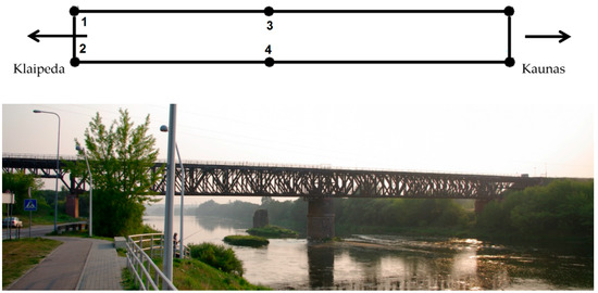
Figure 2.
Layout of the points of measurement in the bridge structure.
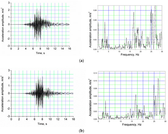
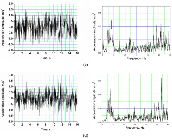
Figure 3.
Vertical vibrations and their spectral density of beams 1 (a,c) and 2 (b,d) of the road overlay, (a,b) during the locomotive movement; (c,d) during the freight train movement.
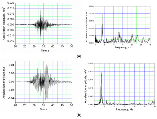
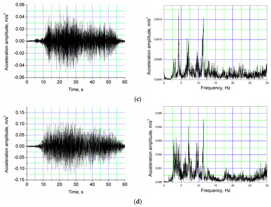
Figure 4.
Vertical (a,c) and longitudinal (b,d) vibrations and their spectral density of the support (filtered vibrations above 30 Hz): (a,b) during the locomotive movement; (c,d) during the freight train movement.
Measurement data arrays were processed using the compiled computer software with Matlab programme package operators.
Since a size (scalar) is the trend of cases of this problem, the following equation is used:
where is the estimate of the standard deviation , which is calculated according to the formula:
The quality of data of all 8 acceleration vectors was assessed at their precision indicator by one standard deviation. Estimates of standard deviations are presented in Table 1.

Table 1.
Shapes and frequencies of bridge overlay vibrations; values of their suppression coefficients.
The results in Figure 3 and Figure 4 show vertical (a,c) and longitudinal (b,d) vibrations and their spectral density of 1, 3 and 4 points (Figure 1) point 1. The spectral density graphs illustrate the change of acceleration amplitudes in the frequency range from 0 to 30 Hz. The analysis of the acceleration amplitudes of vertical direction manifesting at the middle section of the bridge during the running of a locomotive, which are presented in graphs in Figure 3a,b (the graphs show acceleration measurement results at 3 and 4 points (Figure 1)), revealed that the amplitude at 3.25 Hz dominated in the frequency range from 1 to 10 Hz, while the respective analysis of the frequency range from 10 to 30 Hz showed the dominant amplitudes at 16.81, 24.75, 25.06, 26.69 and 26.8 Hz. The analysis of the acceleration amplitudes of vertical direction manifesting at the middle section of the bridge during the movement of a freight train, which are presented in graphs in Figure 3c,d (the graphs show acceleration measurement results at 3 and 4 points (Figure 1)), revealed that the acceleration amplitudes from 2.25 to 3.94 Hz dominated at the frequency range from 1 to 10 Hz, while the respective analysis of the frequency range from10 to 30 Hz showed the dominant amplitudes at 23.88, 26.00 and 27.13 Hz. The analysis of the acceleration amplitudes of vertical and horizontal direction manifesting at the bridge support during the running of a locomotive, which are presented in graphs in Figure 4a,b (the graphs show results of measurement of acceleration at 1 point (Figure 1)) showed that the dominant amplitude was 3.80 Hz in the frequency range from 1 to 30 Hz. The analysis of the acceleration amplitudes of vertical and horizontal direction manifesting at the bridge support during the running of a freight train, which are presented in graphs in Figure 4c,d (the graphs show results of measurement of acceleration at 1 point (Figure 1)) revealed the manifestation of dominant amplitudes in the frequency range from 1 to 11.5 Hz, with significantly dominating amplitudes at 4.25, 7.11 and 11.48 Hz.
Figure 5 illustrates the first shapes of the 5 modes used in the experimental modal analysis, while Table 1 presents the key data of the experimental modal analysis: frequency values of the modes and suppression coefficients for each mode.
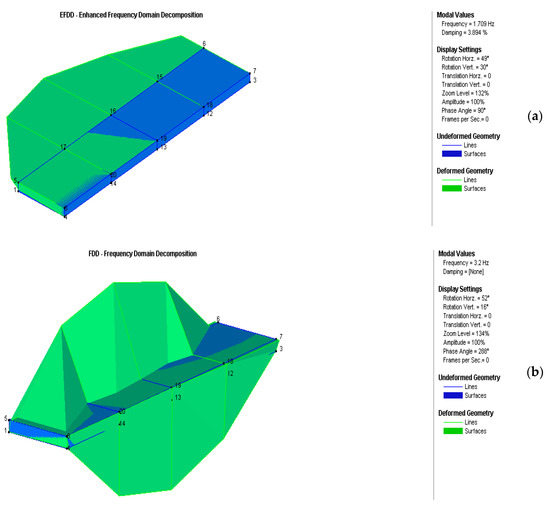
Figure 5.
Shapes of modes received in the experimental modal analysis: (a) horizontal bending—half wave; (b) vertical rotation—half wave; (c) horizontal bending—half wave; (d) vertical rotation—2 half waves; (e) vertical bending—2 half waves.
Table 2 shows Figure 3 and Figure 4; statistical parameters of acceleration values, 1-4 vectors are described in Figure 4, and vectors 5–8 are described in Figure 3. Figure 3 the unfiltered acceleration values o 4 are filtered and filtered at 30 Hz (filtered vibrations above 30 Hz), resulting in this difference.
Table 2.
Precision indicators of acceleration vectors.
4. Covariance Model of Vibration Signal Parameters
In the theoretical model [24,25,26,27], errors of measurement of digital vibration signals are assumed to be random and systematic.
The trend of measurement data of vectors is eliminated in each vector of the arrays of measurement of vibrations parameters. Time interval of dissemination of vibrations is used as one of the parameters.
A random function compiled on the basis of arrays of measurement data of vibration parameters is considered stationary (in the broad sense), i.e., with the average of while the covariance function depends solely on the difference between arguments − Discrete Fourier transformation [16,17,18,19,28,29,30,31,32] may be used to process digital signals. Auto-covariance function of one data array or inter-covariance function of two arrays is expressed as follows [78]:
or
where are the centred measurement vectors of vibration parameters , after the elimination of the trend, u is the vibrations parameter, is the variable quantum interval, k is the number of units of measure, Δ is the value of units of measure, T is time, and M is the symbol of an average.
According to the available vibration parameter measurement data, the covariance function estimate is calculated as follows:
where n is the total number of discrete intervals.
Formula (14) may be applied in the form of an auto-covariance or inter-covariance function. In case of an auto-covariance function, arrays and are parts of individual arrays, and when a function is a covariance function, there are two different arrays.
The estimate of the normalized covariance function is:
where is the estimate of standard deviation of a random function.
The following formulas are used to eliminate the trend of the digital i measurement array vectors:
where is the array of reduced values of i digital array, with eliminated vector trend; − i array of the measured vibration parameters, e is the the only vector measured at (n × 1); n is the number of lines in i array, is the vector of weighted averages of i array vectors, is the j vector of reduced values of i array, j = 1, …, m.
Arithmetic or a weighted average is used to eliminate the vector trend. The vector of arithmetic averages of i array vectors is calculated according to the formula:
The weighted average of vectors is calculated in application of the method of the least squares.
Estimate of covariance matrix of i array of vibration parameters looks as follows:
where array dimensions must be the same.
The accuracy of the calculated correlation coefficient is defined by the standard deviation assessing its value according to the formula
where k => 8000 r is the correlation coefficient. The greatest standard deviation estimate is received when r value is close to zero, then where we have [29,30,31,32,33,34,35,36,37,38,39,40,41].
5. Results of the Analysis of the Vibration Accelerations Model
Eight arrays of data of measurements of vibration accelerations were received using accelerometer 8344. Signals were captured at the following time intervals: and 64 s and 16 s. vibration signal acceleration values were fitted in each vector of the array.
The expression of each measurement vector is a random function for random measurement errors, when, by bringing its expression close to the shape of a stationary function, trend components, which were calculated in application of the method of the least squares, were eliminated.
Values of the quantization interval of the normalized covariance functions range from 1 to . Estimate of the normalized auto-covariance function was calculated for each vector of vibrations and graphical expressions of 8 normalized auto-covariance functions were received.
Estimates of normalized inter-covariance functions were calculated in the same manner according to 8 vectors for both vibrations, and 28 graphical expressions of them were received according to their respective combinations.
All normalized auto-covariance functions for 8 vibration acceleration vectors receive their highest correlation coefficient values at the quantization interval values and further decrease to at for 1–4 vectors and for 5–8 vectors. According to the data of different vectors, the rate of decrease of correlation is different.
Normalized inter-covariance functions have correlation coefficient values close to zero for all pairs of vectors, except , and decrease to at and
Figure 6, Figure 7, Figure 8, Figure 9, Figure 10, Figure 11, Figure 12 and Figure 13 illustrate more significant graphical expressions.
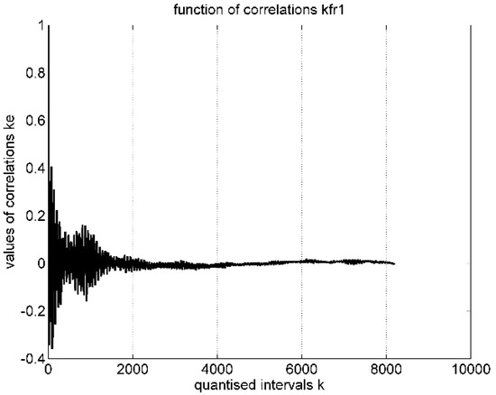
Figure 6.
Normalized auto-covariance function of the 1st vibration accelerations vector.
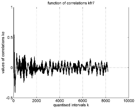
Figure 7.
Normalized auto-covariance function of the 7th vibration accelerations vector.
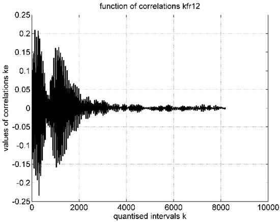
Figure 8.
Normalized inter-covariance function of the 1st and 2nd vibration accelerations vectors.
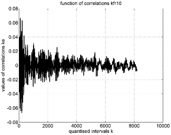
Figure 9.
Normalized inter-covariance function of the 1st and 6th vibration accelerations vectors.
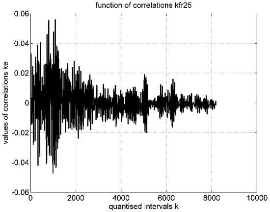
Figure 10.
Normalized inter-covariance function of the 2nd and 5th vibration accelerations vectors.
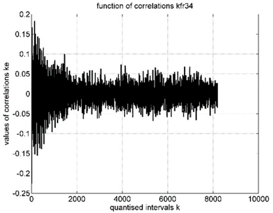
Figure 11.
Normalized inter-covariance function of the 3th and 4th vibration accelerations vectors.
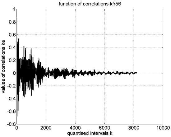
Figure 12.
Normalized inter-covariance function of the 5th and 6th vibration accelerations vectors.
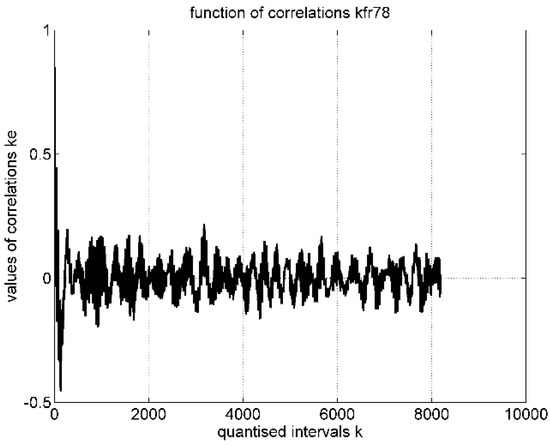
Figure 13.
Normalized inter-covariance function of the 7th and 8th vibration accelerations vectors.
Figure 14 presents a graphical image of the summarized (spatial) correlation matrix of the array of 8 vectors of vibration accelerations. The correlation matrix expression gets a block shape of 8 pyramids, where correlation coefficient values are shown in colour spectrum shades. Colour projections of pyramids are illustrated in the horizontal plane.
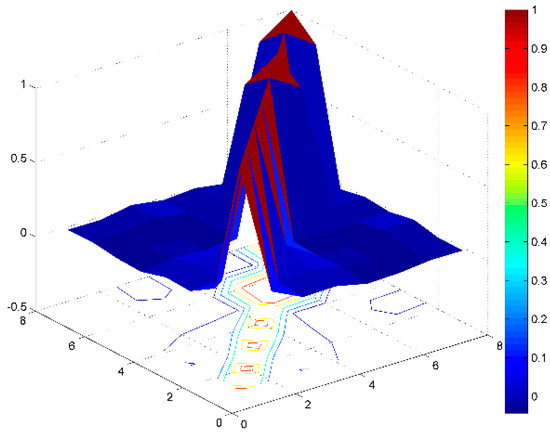
Figure 14.
Graphical image of summarized (spatial) correlation matrix of the array of 8 vectors of vibration accelerations.
Analysis of Figure 6, Figure 7, Figure 8, Figure 9, Figure 10, Figure 11, Figure 12 and Figure 13 made it possible to determine the correlation values between the examined vectors (from Table 1). The results shown in Figure 6 revealed (1st vibration accelerations vector) that the correlation coefficient value varies ±0.4 where ; accordingly, at , the correlation coefficient value changes ±0.2 and with increasing , the correlation coefficient value is . The results of Figure 7 showed (7th vibration accelerations vector) that the correlation coefficient value changes from +0.53 to −0.44 ; accordingly, with increasing , the correlation coefficient value is . The assessment of the results of Figure 8 revealed (1st and 2nd vibration accelerations vectors) that the correlation coefficient value ranges from +0.21 to −0.24 at , and accordingly, at the correlation coefficient value varies ±0.16 and with increasing , the value is . An assessment of the results of Figure 9 revealed (1st and 6th vibration accelerations vectors) that the correlation coefficient value changes ±0.07 at , and with increasing , the correlation coefficient value . The assessment of the results of Figure 10 showed (2nd and 5th vibration accelerations vectors) that the correlation coefficient value ranges from +0.06 to −0.05, when , and with respectively increasing , the correlation coefficient value . An assessment of the results of Figure 11 revealed (3th and 4th vibration accelerations vectors) that the correlation coefficient value ranges from +0.18 to −0.23 at , and with increasing the correlation coefficient value . The analysis of the results of Figure 12 showed (5th and 6th vibration accelerations vectors) that the correlation coefficient value varies from +0.88 to −0.68 at ; accordingly, where , the correlation coefficient value ranges ±0.4 and with increasing , the correlation coefficient value . The assessment of the results of Figure 13 revealed (7th and 8th vibration accelerations vectors) that the correlation coefficient value varies ±0.45 at , and with increasing , the correlation coefficient value .
6. Conclusions
Normalized auto- covariance and inter- covariance functions of vibration signal accelerations of the bridge points allowed us to determine the change in correlation and probability dependence between signal accelerations according to quantization range of signal time.
Values of normalized auto-covariance functions of all acceleration vectors changed from at the quantization interval values and at . The curve of correlation of different vectors differs, thus the probabilistic dependence between the parameters of the same acceleration vector decreased rather slowly over time.
Normalized inter-correlation functions have correlation coefficient values which are close to zero for pairs of vectors of accelerations (vertical and longitudinal) of all points of the bridge overlay, which shows that the structure of bridge trusses is stable enough, and that each node works in individual mode. This assumption was also confirmed by the expressions of normalized auto-covariance functions of 8 acceleration vectors when the rate of their change is individual. However, inter-correlation of 5–8 acceleration vectors is notable when and decreases to at and which shows that acceleration vectors of two beams of the bridge have a probabilistic interconnection having possibly formed due to their structural properties.
The impact which a train has on the bridge was analysed without emphasizing the bridge parameters, determining interdependences of vibration results of points in the bridge structure. Determining said interdependences makes it possible to predict the dynamic results of hard-to-reach points of the bridge structure. The results of this method could be used in structural health monitoring (SHM).
Author Contributions
Conceptualization, A.K. and J.S.; methodology, K.K.; software, J.S.; validation, A.K. and J.M.; formal analysis, J.M.; investigation, A.K.; resources, K.K.; data curation, J.S.; writing—original draft preparation, A.K.; writing—review and editing, K.K. and J.M.; visualization, J.S.
Funding
This research received no external funding.
Acknowledgments
In this section you can acknowledge any support given which is not covered by the author contribution or funding sections. This may include administrative and technical support, or donations in kind (e.g., materials used for experiments).
Conflicts of Interest
The authors declare no conflict of interest.
References
- Ataei, S.; Miri, A. Investigating dynamic amplification factor of railway masonry arch bridges through dynamic load tests. Constr. Build. Mater. 2018, 183, 693–705. [Google Scholar] [CrossRef]
- Skeivalas, J.; Jurevicius, M.; Kilikevicius, A.; Turla, V. An analysis of footbridge vibration parameters. Measurement 2015, 66, 222–228. [Google Scholar] [CrossRef]
- Guchhait, S.; Banerjee, B. Constitutive error based parameter estimation technique for plate structures using free vibration signatures. J. Sound Vib. 2018, 419, 302–317. [Google Scholar] [CrossRef]
- Xia, H.; De Roeck, G.; Goicolea, J.M. (Eds.) Bridge Vibration and Controls: New Research; Nova Science Publisher’s: Hauppauge, NY, USA, 2012. [Google Scholar]
- Xia, H.; Zhang, N.; Guo, W.W. Analysis of resonance mechanism and conditions of train–bridge system. J. Sound Vib. 2006, 297, 810–822. [Google Scholar] [CrossRef]
- Niknam, A.; Farhang, K. Friction-induced vibration due to mode-coupling and intermittent contact loss. J. Vib. Acoust. 2018, 141, 021012. [Google Scholar] [CrossRef]
- Niknam, A.; Farhang, K. Vibration instability in a large motion bistable compliant mechanism due to stribeck friction. J. Vib. Acoust. 2018, 140, 061017. [Google Scholar] [CrossRef]
- Capsoni, A.; Ardito, R.; Guerrieri, A. Stability of dynamic response of suspension bridges. J. Sound Vib. 2017, 393, 285–307. [Google Scholar] [CrossRef]
- Xu, Y.L.; Zhang, N.; Xia, H. Vibration of coupled train and cable-stayed bridge systems in cross winds. Eng. Struct. 2004, 26, 1389–1406. [Google Scholar] [CrossRef]
- Cheng, Y.S.; Au, F.T.K.; Cheung, Y.K. Vibration of railway bridges under a moving train by using bridge-track-vehicle element. Eng. Struct. 2001, 23, 1597–1606. [Google Scholar] [CrossRef]
- Dinh-Cong, D.; Dang-Trung, H.; Nguyen-Thoi, T. An efficient approach for optimal sensor placement and damage identification in laminated composite structures. Adv. Eng. Softw. 2018, 119, 48–59. [Google Scholar] [CrossRef]
- Jin, H.; Xia, J.; Wang, Y. Optimal sensor placement for space modal identification of crane structures based on an improved harmony search algorithm. J. Zhejiang Univ. Sci. A 2015, 16, 464–477. [Google Scholar] [CrossRef]
- Leitold, D.; Vathy-Fogarassy, A.; Abonyi, J. Network distance-based simulated annealing and fuzzy clustering for sensor placement ensuring observability and minimal relative degree. Sensors 2018, 18, 3096. [Google Scholar] [CrossRef] [PubMed]
- Lenticchia, E.; Ceravolo, R.; Antonaci, P. Sensor placement strategies for the seismic monitoring of complex vaulted structures of the modern architectural heritage. Shock Vib. 2018, 2018, 3739690. [Google Scholar] [CrossRef]
- Lian, J.; He, L.; Ma, B.; Li, H.; Peng, W. Optimal sensor placement for large structures using the nearest neighbour index and a hybrid swarm intelligence algorithm. Smart Mater. Struct. 2013, 22, 095015. [Google Scholar] [CrossRef]
- Muthuraman, U.; Hashita, M.M.S.; Sakthieswaran, N.; Suresh, P.; Kumar, M.R.; Sivashanmugam, P. An approach for damage identification and optimal sensor placement in structural health monitoring by genetic algorithm technique. Circuits Syst. 2016, 7, 814–823. [Google Scholar] [CrossRef]
- Qin, B.Y.; Lin, X.K. Optimal sensor placement based on particle swarm optimization. Adv. Mater. Res. 2011, 271–273, 1108–1113. [Google Scholar] [CrossRef]
- Yi, T.-H.; Li, H.-N.; Gu, M. Optimal sensor placement for structural health monitoring based on multiple optimization strategies: OSP for SHM based on multiple optimazation strategies. Struct. Des. Tall Spec. Build. 2011, 20, 881–900. [Google Scholar] [CrossRef]
- Plachý, T.; Polák, M.; Ryjáček, P. Assessment of an old steel railway bridge using dynamic tests. Procedia Eng. 2017, 199, 3053–3058. [Google Scholar] [CrossRef]
- Zhang, B.; Ding, X.; Werner, C.; Tan, K.; Zhang, B.; Jiang, M.; Zhao, J.; Xu, Y. Dynamic displacement monitoring of long-span bridges with a microwave radar interferometer. ISPRS J. Photogramm. Remote Sens. 2018, 138, 252–264. [Google Scholar] [CrossRef]
- Cantero, D.; Arvidsson, T.; OBrien, E.; Karoumi, R. Train–track–bridge modelling and review of parameters. Struct. Infrastruct. Eng. 2016, 12, 1051–1064. [Google Scholar] [CrossRef]
- Horas, C.S.; Alencar, G.; De Jesus, A.M.P.; Calçada, R. Development of an efficient approach for fatigue crack initiation and propagation analysis of bridge critical details using the modal superposition technique. Eng. Fail. Anal. 2018, 89, 118–137. [Google Scholar] [CrossRef]
- Mirza, O.; Kaewunruen, S.; Dinh, C.; Pervanic, E. Numerical investigation into thermal load responses of railway transom bridge. Eng. Fail. Anal. 2016, 60, 280–295. [Google Scholar] [CrossRef]
- Beijen, M.A.; Heertjes, M.F.; Butler, H.; Steinbuch, M. Disturbance feedforward control for active vibration isolation systems with internal isolator dynamics. J. Sound Vib. 2018, 436, 220–235. [Google Scholar] [CrossRef]
- Jurevicius, M.; Turla, V.; Bureika, G.; Kilikevicius, A. Effect of external excitation on dynamic characteristics of vibration isolating table. Eksploat. Niezawodn. Maint. Reliab. 2015, 17, 260–265. [Google Scholar] [CrossRef][Green Version]
- Koch, K.-R. Einführung in Die Bayes-Statistik; Springer: Berlin/Heidelberg, Germany, 2000. [Google Scholar]
- KilikevičIenė, K.; Skeivalas, J.; KilikevičIus, A.; PečEliūNas, R.; Bureika, G. The analysis of bus air spring condition influence upon the vibration signals at bus frame. Eksploat. Niezawodn. Maint. Reliab. 2015, 17, 463–469. [Google Scholar] [CrossRef]
- Reju, S.A.; Kgabi, N.A. Wavelet analyses and comparative denoised signals of meteorological factors of the Namibian atmosphere. Atmos. Res. 2018, 213, 537–549. [Google Scholar] [CrossRef]
- Song, M.-H.; Li, K.-H.; Kim, S.-N. Evaluation of periodicities and fractal characteristics by wavelet analysis of well log data. Comput. Geosci. 2018, 119, 29–38. [Google Scholar] [CrossRef]
- Afzal, P.; Ahmadi, K.; Rahbar, K. Application of fractal-wavelet analysis for separation of geochemical anomalies. J. Afr. Earth Sci. 2017, 128, 27–36. [Google Scholar] [CrossRef]
- Makieła, W.; Gogolewski, D. Variability evaluation of signal in two-dimensional wavelet decomposition using fractal dimension. Procedia Eng. 2017, 192, 243–248. [Google Scholar] [CrossRef]
- Zhao, L.; Bai, H.; Liang, J.; Wang, A.; Zeng, B.; Zhao, Y. Local activity-driven structural-preserving filtering for noise removal and image smoothing. Signal Process. 2019, 157, 62–72. [Google Scholar] [CrossRef]
- Che, L.; Xiao, W.; Pan, F.; Dong, B.; Zhong, Z. Reduction of speckle noise in digital holography by combination of averaging several reconstructed images and modified nonlocal means filtering. Opt. Commun. 2018, 426, 9–15. [Google Scholar] [CrossRef]
- Liu, S.; Rahman, M.A.; Liu, S.C.; Wong, C.Y.; Lin, C.-F.; Wu, H.; Kwok, N. Image de-hazing from the perspective of noise filtering. Comput. Electr. Eng. 2017, 62, 345–359. [Google Scholar] [CrossRef]
- Singh, P.; Shree, R. A new SAR image despeckling using directional smoothing filter and method noise thresholding. Eng. Sci. Technol. Int. J. 2018, 21, 589–610. [Google Scholar] [CrossRef]
- Duan, Y.; Liu, F.; Jiao, L.; Zhao, P.; Zhang, L. SAR image segmentation based on convolutional-wavelet neural network and markov random field. Pattern Recognit. 2017, 64, 255–267. [Google Scholar] [CrossRef]
- Bianchi, T.; Argenti, F.; Lapini, A.; Alparone, L. Amplitude vs. intensity bayesian despeckling in the wavelet domain for SAR images. Digit. Signal Process. 2013, 23, 1353–1362. [Google Scholar] [CrossRef][Green Version]
- Mukhopadhyay, P.; Chaudhuri, B.B. A survey of Hough transform. Pattern Recognit. 2015, 48, 993–1010. [Google Scholar] [CrossRef]
- Cha, J.; Cofer, R.H.; Kozaitis, S.P. Extended Hough transform for linear feature detection. Pattern Recognit. 2006, 39, 1034–1043. [Google Scholar] [CrossRef]
- Yin, G.; Li, A.; Wu, S.; Fan, W.; Zeng, Y.; Yan, K.; Xu, B.; Li, J.; Liu, Q. PLC: A simple and semi-physical topographic correction method for vegetation canopies based on path length correction. Remote Sens. Environ. 2018, 215, 184–198. [Google Scholar] [CrossRef]
- Zhao, B.; Wu, J.; Yang, F.; Pilz, J.; Zhang, D. A novel approach for extraction of gaoshanhe-group outcrops using landsat operational land imager (OLI) data in the heavily loess-covered Baoji district, Western China. Ore Geol. Rev. 2019, 108, 88–100. [Google Scholar] [CrossRef]


© 2019 by the authors. Licensee MDPI, Basel, Switzerland. This article is an open access article distributed under the terms and conditions of the Creative Commons Attribution (CC BY) license (http://creativecommons.org/licenses/by/4.0/).