1. Introduction
In order to expand the coverage of wireless networks and improve the communication quality of edge users, relay has been widely used in wireless networks such as long term evolution (LTE) and 5G [
1,
2]. However, dense deployment of relays can lead to problems such as high energy consumption and greenhouse gas emissions [
3,
4]. Energy harvesting technology is the most promising technology to solve the economic and environmental problems caused by the dense deployment of relays, which can collect and utilize renewable energy such as solar and wind energy [
5,
6,
7,
8,
9]. In addition, energy harvesting technology can reduce the dependence of wireless networks on grid energy. Deploying green relays in areas where grid energy is scarce can effectively expand the coverage of wireless communication networks. However, the intermittent and random nature of the renewable energy may cause a decline in network performance. Therefore, it is critical to establish a renewable energy allocation and link selection mechanism to ensure the performance of wireless relay networks.
Optimal power control strategies to alleviate network performance degradation caused by the lack of renewable energy have been proposed in [
10,
11,
12,
13]. In [
10], both the source and relay nodes are powered by renewable energy, and an off-line power control strategy is made to minimize data transmission time with throughput constraints. It was also proved that the power control strategy has water injection structure. Differing from [
10], literature [
11] considered how the source node is powered by the grid while the relay node is powered by renewable energy. An off-line power control strategy is proposed to maximize the grid energy efficiency of the source node. In [
12], the research was extended to a Gauss fading channel, with both off-line and on-line power control schemes are proposed. In addition to the traditional relay, the literature [
13] considers the relay with cache function. Off-line and on-line power control strategies are developed to maximize network throughput. All of the above studies have developed off-line or on-line power control strategies under the constraints of user’s quality of service (QoS).
Besides power control schemes, link selection strategies are also critical. In [
14], the source node is powered by grid energy while the relay is powered by renewable energy. With causal side information, a link selection strategy is made to maximize the average throughput of all time slots. In [
15], the relay is powered by radio frequency (RF) energy with a finite battery capacity, and only one data packet needs to be transmitted in each slot. A link selection scheme based on battery level is proposed to minimize the outage probability of the relay. Further, literature [
16] jointly optimizes power and link selection to reduce outage probability of the relay. In [
17], the research was extended to multi-relay with data caching, Under the constraints of battery capacity, on-line and off-line power allocation and link selection mechanisms were developed to minimize data transmission time.
Most previous studies on hybrid energy supply (HES) wireless relay systems assume that the amount of data transmitted by the source node are fixed in each slot, and then optimize the outage probability or transmission time. However, in practical applications, the source node needs to serve a lot of different users and deliver unfixed data bits in each slot. So, data bits should be transmitted as much as possible to reduce the network congestion with grid energy consumption constraints. Consequently, in this paper, we consider that the source node has available bits to be transmitted all the time. Our goal is to maximize network throughput while minimizing grid energy consumption.
The rest of this paper is organized as follows.
Section 2 describes the system model. In
Section 3, the Markov decision process (MDP) problem is formulated, for which a low-complexity algorithm is proposed. Simulations are shown in
Section 4. Finally,
Section 5 highlights the conclusion.
3. Optimal Control for Expected Total Rewards
In this section, we assume
,
and
are causally known. Consequently, we aim to adapt the transmission power and link selection to maximize the expected total rewards. Thus, the problem can be formulated as:
In , the objective is the expected total rewards over N time slots. Equation (12) is the energy constraint that the energy consumed by relay should not exceed that of the battery. Equation (13) is the throughput constraint that the bits delivered in the two stages of relay link should be Equations (14) and (15) are the power constraint and the link selection constraint.
3.1. Problem Simplification
From Equation (10), we can see that the optimized variables of
include the 0–1 variable
and the continuous variable
,
and
. Thus, it is very difficult to optimize so many different types of variables at the same time. Therefore, we do some simplification of
to reduce the optimized variables. And, the problem of
can be expressed as:
And
is the 0–1 variable, which can be calculated as:
That is, when the transmission power of relay is non-zero,
and relay link is chosen to transmit data. While the power of relay is zero,
and direct link is selected to deliver bits. In addition,
is the network total reward when relay link is chosen, which is given by:
where
is the throughput, and
is the grid energy consumed by the source node. We assume that the amount of data bits transmitted in the two stages of relay link should be equal. So, there is
From equation (21), we can know that
According to Equation (20) to (22),
can be further given as:
is the reward when direct link is selected, and the problem of solving
can be expressed as:
Proposition 1. The reward of the direct link is convex in transmission power .
Proof: The second derivative of formula (24) is
which means that
is a convex function. □
According to the properties of convex functions, we can easily know that gets the maximum value at . Therefore, the optimal and are known once is given. However, has practical significance only on [0, ] in this work. Consequently, when , decreases monotonously on [0, ] with maximum value . While , increases monotonously on [0, ] with maximum value .
It can be seen from Equation (16) to (26), that the values of and are determined by , and the maximum value of is a fixed value in each time slot which is only related to . Therefore, the optimal variable of problem is only .
3.2. MDP Model for Expected Total Rewards
Our goal is to maximize the total rewards over N slots through a relay power control scheme. However, due to the limited battery capacity, the relay power selection results in each slot will affect the initial battery capacity at the next moment. So, power decisions on different time slots are mutually influential. The MDP is a useful model to handle such decision problems, and backward induction is an effective algorithm to solve this problem [
24].
Therefore, we formulate
as a Markov decision process (MDP) problem, which can also be expressed as:
where
is a feasible relay power policy,
denotes the set of all feasible policies.
is the reward of slot i, which is given by
.
3.2.1. MDP Basics
A sequential decision-making method is the selection of one of several action strategies in each time slot during the operation of the system [
25]. In the sequential decision process, if the transfer of the system state obeys the known probability law and is independent of the previous history, then this sequential problem is called an MDP problem [
26]. An MDP model consists of a reward function, system states, actions, state transition probability and objective, each of which will be described in detail later.
3.2.2. Reward Function
In an MDP model, the reward function is defined as
. It indicates that the system gets the reward with action
at state j [
27]. This is denoted
as the rule for selecting relay power in slot i. Thus, the rules over N slots can be expressed as
, and the set of all possible rules is denoted as
. Given the initial state k and strategy
, the expected total rewards can be also written as:
where
and
are the states of the relay system and the selected action in the slot i, respectively.
is the conditional probability of using strategy
, starting from state k, selecting action
, and moving to state j at slot
. Our aim is to find the optimal action selection scheme as
, which makes
the maximum value.
3.2.3. Discretization of System States and Actions
The optional values of the system states and actions should be finite in MDP model. However, the system states include links and the battery states, and the relay power actions are continuous values in the wireless relay network. Therefore, it is necessary to discretize the system states and relay power actions. The relay system states consist of channel fading values and battery levels, which can be given as
. We discretize the channel states by reference to the method in literature [
28]. Denoting
as the set of channel fading values, which is an equal-difference sequence. The probability when the channel fading is
with
can be calculated as:
We divide the battery into M + 1 energy level. And the battery states set is taken as
. The real-time energy level of the battery can be calculated by
Denote
as the action set, which is also an equal-difference sequence. Actually, the value of the relay transmit power is constrained by the battery level. Thus, the action set is given as
, where
is calculated by:
is the function that rounds the variable x down.
3.2.4. State Transition Probability
After action
is selected, the system states will migrate from
to
, which can be expressed as
. Since the value of channel fading is equal probability, the state transition probability is:
We assume that
and
are in the
and
levels of the battery, which should satisfy the Equation:
. As mentioned in
Section 2.2, the energy harvesting process obeys the Poisson distribution with mean λ. Therefore, Equation (32) can be further given as:
where
and
is given as
and
, respectively.
is the function that rounds the variable x up.
3.3. The Backward Induction Algorithm for MDP Problem
The backward induction algorithm is an effective solution to the optimal strategy and value function in the finite-stage Markov decision programming problem [
26]. A new function,
, was proposed based on the backward induction algorithm, which is formulated as:
where
[
26]. According to Equation (34), the optimal value function of the expected total rewards can be calculated as
. Meanwhile, the decision sequence
obtained is the optimal strategy.
With the backward induction algorithm, the number of states required to traverse is
. The state space may be very large if some of the elements are of large size and may encounter the curse of dimensionality [
29]. An effective method to reduce the computational complexity in MDP model is proposed in literature [
28]. In this case, we also eliminate some states that do not need to be searched according to the wireless relay network properties in our model by reference [
28].
Proposition 2. When , , are fixed value, and the optimal action is at state , the optimal action is for any state of .
Proof: If the optimal action for the state
is
, according to Equation (34), we know that:
From Equation (21), we know that
Which becomes larger as
grows. Therefore, for any state
with
,
. Since
,
and
are fixed value, we can get
and
Finally,
which proves that the optimal action is
in the state
. □
Proposition 3. When , , are fixed value, and the optimal action is at state , the optimal action is for any state of .
Proof: If the optimal action for state
is
, according to Equation (34), we can get:
While
,
is given as
which becomes smaller as
grows. Thus, For the stat
with
,
. Since
,
and
are fixed value, there are:
and
Finally,
which indicates that the optimal action is
in the state
.
| Algorithm 1. Backward Induction Algorithm Based on States Elimination |
| Input: , , , , , , , , , , , , , , |
| Output: |
| 1: Initialize , |
| 2: While N |
| 3: , ; |
| 4: For m = 1 to M, = 1 to K |
| 5: = K, = 1; |
| 6: While , |
| 7: ; |
| 8: For j = 1: length () |
| 9: Calculate ; |
| 10: End For |
| 11: If |
| 12: , ; |
| 13: = − 1, = + 1; |
| 14: Else |
| 15: if = K |
| 16: = − 1, = 1; |
| 17: Else |
| 18: = + 1; |
| 19: End If |
| 20: End If |
| 21: End For |
| 23: N = N − 1; |
| 24: End While |
4. Numerical Simulations
In this section, we run some numerical simulations to analyze the total reward, grid energy consumption and throughput in two-hop wireless relay networks. In the simulations, we set B = 10 MHz, T = 1 ms,
= 2 W,
= 0.5 W,
= −97.5 dBm,
= −40 dB,
= 4 [
28]. And
= 0.01 mJ,
= 1.6 mJ, K = 10, L = 20,
= 80 m,
. The detailed numerical results are shown as follows.
4.1. Baseline Schemes
Joint Power Control and Link Selection Algorithm (JPLA): The JPCALSA only considers the current system state, and calculates the maximum rewards of relay and direct link, respectively. Then, the optimal access link is selected by comparing the rewards.
Power Control Algorithm (PCA): The PCA is to maximize the reward in single slot by adjusting the power of the relay, and link selection scheme is not taken into account [
11].
When the energy of relay is sufficient, the system will be in the ideal state. In order to compare the ideal results with our results in different situations, we propose JPLA-F and BIABoSE-F, which are JPLA and BIABoSE with enough renewable energy.
4.2. Parameter Analysis
Figure 2 demonstrates the total rewards with different number of battery levels at different time slots. In any slot, the total rewards increase with the number of battery levels rises. Actually, the energy between two adjacent levels is expressed by the lower level, and the interval of two adjacent levels is smaller as the number of levels becomes larger. At this point, the error between the true value and the expressed value will be smaller, which makes a more accurate result. When the number of battery levels reach 80 and 160, their rewards are close and maximal. Consequently, for reducing the computational complexity, M = 80 is used for simulation analysis in the follow-up.
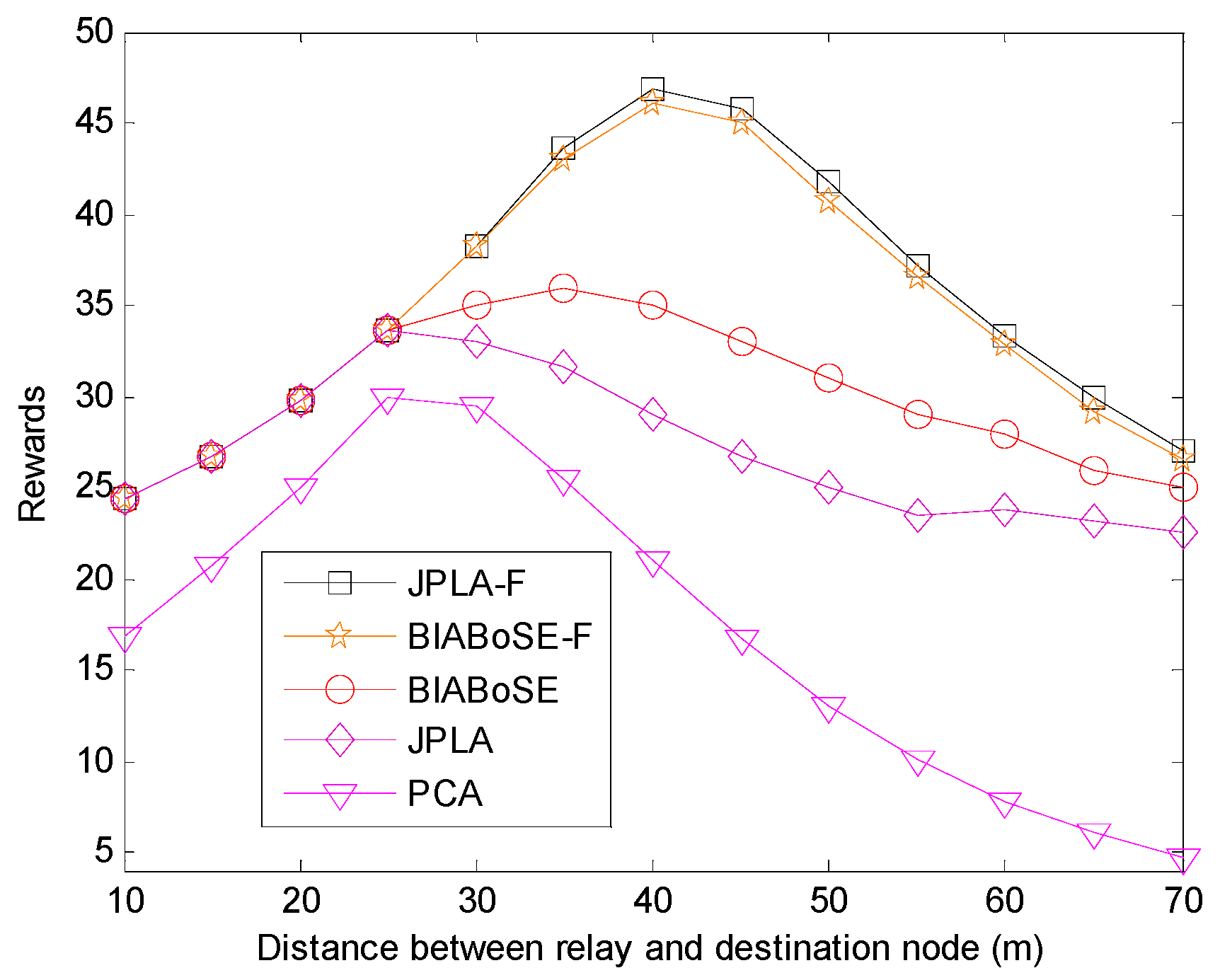
We assume that
, and the total rewards vary with
is shown in
Figure 3 and
Figure 4. As
increases, the rewards of all algorithms become larger first and then decrease. When
is small,
is large, and the path loss between the source node and relay is high. In this case, the source node delivers a few bits to relay with high grid energy consumption, which leads to low total rewards. As
increases, the path loss between the source node and relay decreases, and the total rewards rise. Once
is larger than a certain threshold, the path loss between the relay and destination is high, the number of bits that can be transmitted by relay is lower than that by source node. In this case, the total reward is gradually reduced as the throughput of relay tapers off.
In addition, the JPLA-F and BIBAoSE-F achieve the maximum value near = 40 m in both Figures. Meanwhile, the PCA, JPLA and BIBAoSE obtain the maximum value at different in two Figures. Unlike the JPLA-F and BIBAoSE-F, the other three algorithms are affected by the energy harvesting intensity. The energy that the relay needed for data transmission grows larger as increases. Therefore, when the energy is more sufficient, the total rewards will be closer to optimal result. The total rewards reach the maximum value at = 40. Thus, we choose = 40 for subsequent simulations to better observe the improvement of system performance in the absence of energy.
4.3. Total Reward Maximization
Figure 5 shows the total rewards changes with the time slots. Compared with the PCA, the JPLA adds a link selection mechanism. Therefore, the JPLA can transmit data through the direct link when the battery is very low, which can increase the total rewards. The BIBAoSE takes the future system states into account, which makes a more efficient green energy allocation over N slots than the JPLA. However, all the algorithms can only alleviate the system performance degradation caused by insufficient energy and cannot replace the green energy supply. Therefore, the JPLA-F and the BIBAoSE-F always have the highest total rewards.
Figure 6 displays the total rewards vary as energy harvesting intensity increases. The system is in a green energy-deficient state, when the energy intensity is low. In this case, the relay can deliver more bits as the intensity increases, which leads to a higher reward. However, the rewards will be constant once the energy intensity reaches a certain threshold, because the battery capacity is limited. It should be noted that the rewards of the BIABoSE are lower than the other algorithms when the green energy is enough due to the discretization of states. However, the BIABoSE achieves better performance in our main application scenario, which is a lack of green energy.
4.4. Grid Energy Consumption and Throughput Trade-Off
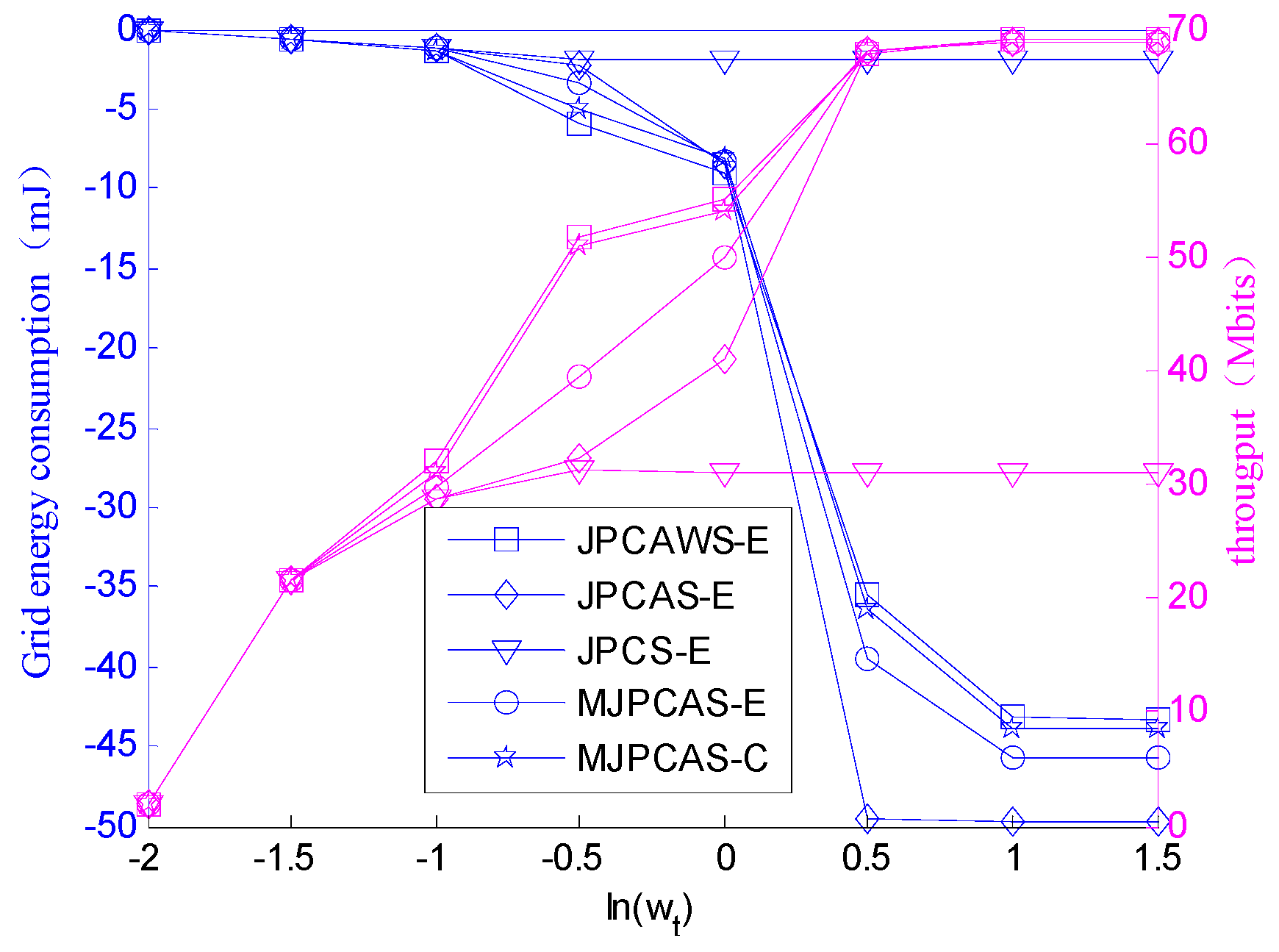
Figure 7 shows the grid energy consumption and throughput when
takes different values. When
is very small, the energy consumption and throughput of all schemes are similar. In this case, the system has a high demand for grid energy consumption, which will impose strict limits on energy consumption. When
increases, the throughput plays an increasingly important role in the reward. Although our schemes consume a little more energy than the JPLA and PCA, it greatly improves the throughput. When the value of
is large, all schemes pursue maximum throughput regardless of energy consumption costs. Therefore, all throughput gains are very close. However, the BIBAoSE consumes the least energy and is closest to the JPLA-F and BIBAoSE-F. In addition, once the throughput constraints are given, we can find the value of
and get the minimum grid energy consumption.
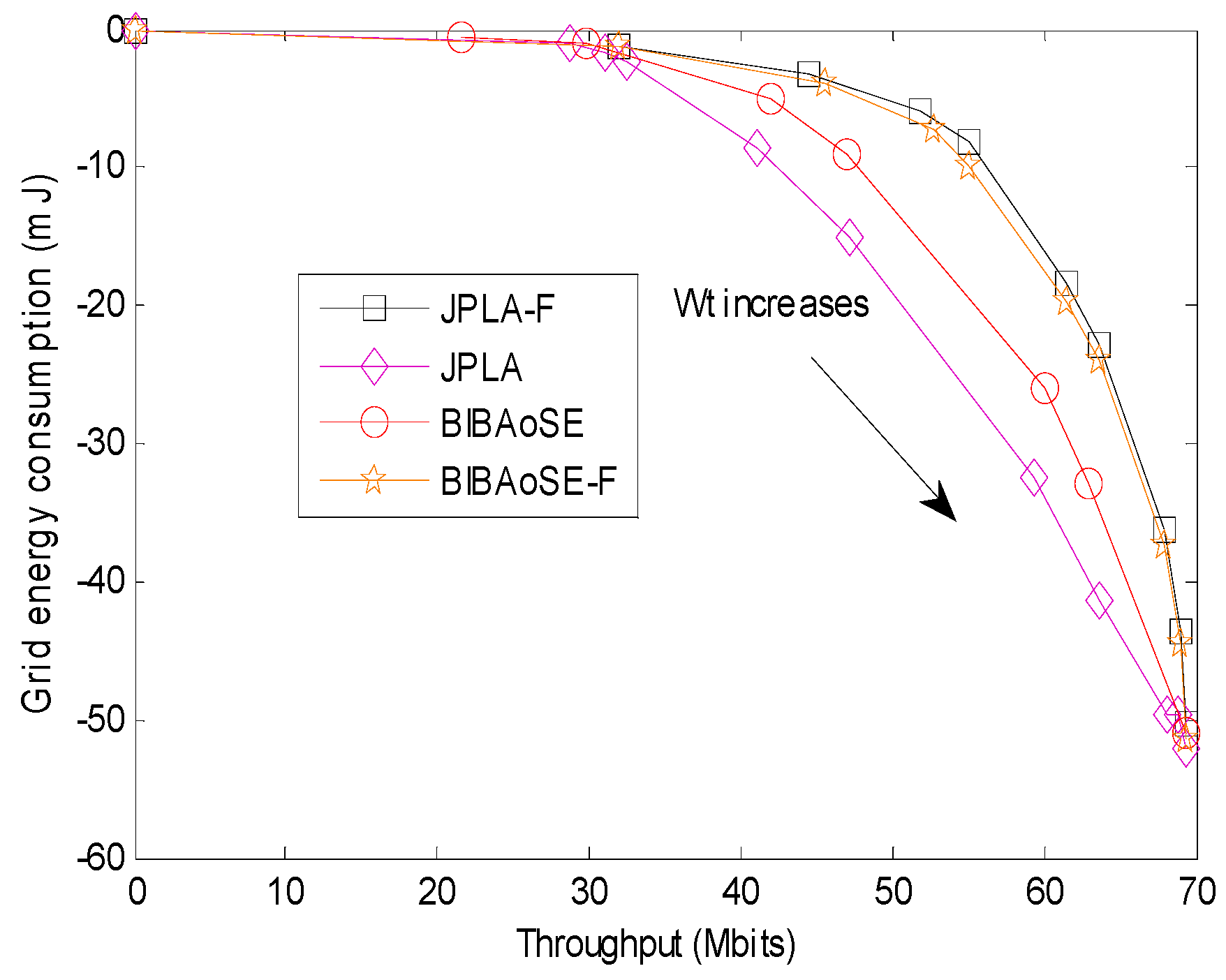
The energy consumption and throughput are shown in
Figure 8. As can be seen from the graph, the BIBAoSE consumes less grid energy than the JPLA when achieves the same throughput. And the BIBAoSE can transmit more bits than the JPLA with the same grid energy supply. In short, the BIBAoSE has a better trade-off between energy consumption and throughput, which is closer to the ideal situation such as the JPLA-F and BIBAoSE-F.


