A Hybrid Model for Investigating the Effect of Scattering from Building Façade on Sound Propagation in Street Canyons

Featured Application

The model developed in this study can be directly used for noise propagation simulation in urban areas, which can be further used for noise control and the prediction of the social response to noise.

Abstract

Street canyons are basic components of modern cities. Sound propagation in streets has been proven to be significantly affected by reflections from building façades. In this paper, an iterative model combining acoustic radiosity and the image source method (IMCRI) is proposed to investigate the effect of diffuse reflections on sound propagation in urban street canyons. By applying image patches, this model calculates both specular reflected components and diffuse reflected components in every reflection. The accuracy of this model is then validated with full-scale measured data from five actual streets with different scattering conditions. Good agreements of sound pressure level and reverberation time are found between the IMCRI and the measurements. The performance of the IMCRI is found to be superior to those of the existing energy models, especially for the reverberation time simulation.

1. Introduction

Noise is one of the problems that has arisen in modern cities and has been shown to have a significant influence on people’s life quality, such as speech interference [1], annoyance [2,3], sleep disturbance [4] and further health effects [5,6,7]. In recent years, many studies have been conducted to prevent people from being impacted by noise. Noise barriers are the most common measures for noise reduction, and the influences of green roofs and building façades are also examined [8,9,10]. To assess the sound environment or apply possible noise control measures, it is essential to have accurate calculation methods for simulating sound propagation in urban areas; however, unfortunately, this has not yet been fulfilled.

Various calculation models have been used to investigate the influential factors of noise propagation in urban streets, which can be classified into three groups: wave-based models [11,12], diffusion equation models [13], and geometrical acoustic (GA) models [14,15]. Because of the time efficiency, the GA models have been widely applied to investigate the fundamental principles of sound propagation in streets, including the image source model (ISM) [16], ray tracing model (RTM) [17], acoustic radiosity model (ARM) [18] and hybrid models based on these models [19,20]. In the early studies, building façades and the ground are assumed to be perfectly smooth by the ISM, which has contributed to the fundamental understanding of the behavior of the sound field in streets [16]. However, there are inevitable diffuse reflections due to irregularities in building façades in actual streets, which lead to considerable errors [21]. To simulate the diffuse reflections, RTM and ARM have been widely used. In RTM and corresponding hybrid models, a random process is commonly applied to model the scattered sound. A random number between {0,1} is compared with the scattering coefficient to decide whether a reflection is specular or diffuse [22]. Therefore, a large number of sound rays are needed to obtain an approximation, which leads to a great time cost when simulating sound propagation in large urban spaces. To simulate the diffuse reflection process, the radiosity method was introduced from the field of thermodynamics [23]. By dividing the surfaces into smaller patches, it converts the diffuse reflection on surfaces into energy transfer among patches. Due to the simple geometry of street canyons, ARM is easy to apply and useful in revealing the fundamental differences between sound fields formed by diffusely reflecting boundaries and geometrically reflecting boundaries [18,24].

The original ARM considers only diffuse reflections, which is in contrast to the image source method (ISM) [25]. However, the actual building façades act between these two extreme conditions, which are neither completely diffuse nor completely specular [19]. Therefore, a series of hybrid models were proposed by merging the image source model (ISM) with the radiosity model [19,20,26]. The major problem related to the hybrid model is how different methods are merged to cover all the reflection components. In the hybrid model proposed by Ismail and Oldham, the entire sound energy transfer process was modeled by multiple consecutive specular reflections and the first-order diffuse reflection [26]. Then, in Onaga’s model [19] and Meng’s model [20], high-order diffuse reflections were considered. A similarity among these models is that the entire sound energy transfer is divided into two separate parts: a specular reflected component and a diffusely reflected component. The pure specular reflected component is first modeled by the ISM, and the received energy of each patch is saved as the initial energy for the following diffusely reflected component modeled by ARM. As suggested by Ismail, this scheme could lead to considerable errors with the increase of the scattering coefficient and reflection order, especially for acoustic parameters determined by high-order reflections [26].

Another key problem is model validation, especially in actual street canyons. Due to the complexity of real urban areas, only a few measurements have been implemented [27,28,29,30]. Furthermore, it is difficult to use the measured data directly for model validation because of the lack of accurate parameters of surfaces, especially scattering coefficients. It is common to use a series of hypothetical scattering coefficients in calculation models, and the result is a range of acoustic indexes, such as sound level attenuation. Therefore, model validation can only prove that the measured data is in the range of the simulation result instead of analyzing the detailed accuracy of the calculation model. This leads to difficulties in applying the model in actual street canyons with many surface conditions. A scale model has been developed and widely used to study sound propagation in street canyons [31,32,33,34,35,36]. However, because of the difficulty in reproducing the full-scale phenomena using scale models (due to absorption, scattering, etc.), scale models are also challenging to use to examine the accuracy of a calculation model.

In this paper, an iterative model combining the radiosity method and image source method (IMCRI) is developed that allows both diffuse reflection and specular reflection in any reflection order. Measurements in five actual streets with different building façades are then carried out to investigate the accuracy of the calculation model. Section 2 describes the construction of the IMCRI. In IMCRI, the ARM and ISM were used to model the diffuse reflection and specular reflection, respectively. As a combination, the image patch was applied to calculate the energy transfer by diffuse reflections after specular reflections. Section 3 describes the full-scale measurement in five streets with different building façades for model validation. In the final part of this paper, a comparison between IMCRI and measured data on both sound attenuation along the streets and the sound decay curve is carried out to analyze the model accuracy. Moreover, the comparison between IMCRI and existing models is also carried out to show the improvement of IMCRI by considering the full reflection component.

2. Calculation Model

In this iterative model combining the radiosity method and image source method (IMCRI), street canyons were modeled as uniform rectangles with limited lengths. Sound energy transferred to the upper side and the end of the streets was assumed to be absorbed. The surfaces were divided into small patches (2 × 2 m). The calculation model was implemented as an iterative model, where each iteration models all of the sound energy transferred after a diffuse reflection occurs. For each iteration, the received energy of each receiver position was calculated and stored in a matrix with a time factor. With the increase in the reflection order, the received energy converged toward the full impulse response that was used to calculate the acoustic parameters.

Figure 1 shows the schematic diagram of the sound transfer path and the structures of IMCRI and existing hybrid models (EHM). The sound energy was first emitted from the source to each patch and then separated into two independent components: the specular reflected energy and the diffuse reflected energy. The specular reflected energy could be modeled easily by the ISM, while the diffuse reflected energy was saved as patch sources for the next sound energy transfer modeled by ARM. The process in the 1st reflection was the same in IMCRI and EHM. The difference between IMCRI and EHM began in the 2nd reflection. As shown in Figure 1b, the entire sound propagation was modeled in EHM by a specular reflection process (modeled by the ISM) and a diffuse reflection process (modeled by the ARM). Figure 1c shows the full sound transfer path, where the red line and blue line represent the components calculated by ISM and ARM in EHM, respectively. As the order increased, there were more neglected components in EHM. Only 75% and 50% of the components were calculated in the 2nd reflection and in the 3rd reflection, respectively. It could lead to considerable errors with the increase in the reflection order, especially for acoustic parameters determined by the high-order reflections [26]. This problem was solved by applying ‘Image source’ in IMCRI, as shown in Figure 2. By creating the image sources of patches, the subsequent specular reflected energy after diffuse reflections, the ‘D-S’ and ‘D-S-S’ paths in Figure 1c, were calculated. The ‘D-S-D’ path was then calculated by ARM in the next iteration. Therefore, all sound transfer paths were considered in the IMCRI.

The energy emitted from an image source is calculated as follows:

$$E_{imagesourc{e}_n}=E_{source}{\displaystyle \prod }_{i=1}^n\left(1-{\alpha }_i\right)·\left(1-s_i\right)$$

(1)

where ${\alpha }_i$ and $s_i$ are the absorption and scattering coefficients of the surface where the reflection occurs, respectively. Moreover, $E_{source}$ and $E_{imagesourc{e}_n}$ represent the energy of the source and that of the nth order image source, respectively.

The sound intensity created by a point source (sound source and image sources) $I$ can be calculated as follows:

$$I=\frac{E_{Source}}{4\pi d^2}$$

(2)

Therefore, the received energy of a patch $E_{received}$ can be calculated as follows:

$$E_{received}={\displaystyle \int }\frac{cos\theta }{4\mathsf{\pi }{d}^2}·d{S}_j·E_{source}$$

(3)

The specular reflected part of the received energy can be modeled by the image source method. Moreover, the diffuse reflected part is stored as the starting energy of the diffuse energy transfer process, which can be expressed as follows:

$$E_{patch}=E_{received}·\left(1-{\alpha }_i\right)·s_i$$

(4)

With respect to the directional distribution of the scattering energy, it was assumed that the diffuse reflected sound energy follows the Lambert cosine law, which has been widely used in different models [15,17,19,37]. With the Lambert cosine law, the sound energy transfer between two patches is independent of the incident angle, which could significantly improve the time efficiency. As shown in Figure 2, the sound energy transfer from $Patc{h}_i$ to $Patc{h}_j$, namely Form Factor, can be calculated as follows:

$$E_{receive{d}_j}=\underset{S_i}{\overset{}{{\displaystyle \int }}}\underset{S_j}{\overset{}{{\displaystyle \int }}}\frac{cos{\theta }_i·cos{\theta }_j}{\mathsf{\pi }{d}_{ij}{}^2}d{S}_{i}d{S}_j·E_{patc{h}_i}$$

(5)

where, $E_{receive{d}_j}$ and $E_{patc{h}_i}$ are the energy received by $Patc{h}_j$ and the energy emitted from $Patc{h}_i$, respectively.

The sound energy emitted from an image patch source can be calculated as follows:

$$E_{imagepatc{h}_{i,n}}=E_{patc{h}_i}{\displaystyle \prod }_{k=1}^n\left(1-{\alpha }_k\right)·\left(1-s_k\right)$$

(6)

where, $E_{imagepatc{h}_{i,n}}$ and $E_{patc{h}_i}$ are the energy of the nth order image patch and that of the patch source, respectively; and ${\alpha }_k$ and $s_k$ are the absorption coefficient and scattering coefficient in the kth order reflection, respectively,

As shown in Figure 2, the sound energy transfer from an image patch to the patches can be calculated as follows:

$$E_{receive{d}_j}=\underset{S_{i^{\prime }}}{{\displaystyle \int }}\underset{S_j}{{\displaystyle \int }}\frac{cos{\theta }_{i^{\prime }}·cos{\theta }_{j^{\prime }}}{\mathsf{\pi }{d}_{i^{\prime }j}{}^2}d{S}_{i^{\prime }}d{S}_j·E_{imagepatc{h}_{i,n}}$$

(7)

All the sound energy received by the receivers is either from point sources or surface sources. For the point source, which includes the original sound source and image source, the sound intensity at a receiver position can be calculated using Equation (2). The sound intensity due to a patch source can be calculated as follows:

$$I=\frac{E_{patch}}{S_i}·\underset{S_i}{{\displaystyle \int }}·\frac{cos\theta }{\mathsf{\pi }{d}^2}d{S}_i$$

(8)

where, $E_{patch}$ and $S_i$ are the energy and the area of the patch source, respectively; and $\theta$ and $d$ are the incident angle and the distance between the receiver and a point on the surface source, respectively.

Ideally, the accuracy will improve when higher-order reflections and image patches are calculated. However, with the increase in the iteration number, the sound energy calculated will rapidly decrease and the average propagation time will increase. Therefore, the simulation accuracy will not significantly improve by taking into account more reflections when the considered reflection order is very high. Meanwhile, the exponential growth of the number of energy transfer paths can be found with the increase in the number of iterations. Hence, a termination condition is necessary to obtain a balance of accuracy and time costs. In IMCRI, an auto-termination process was applied to stop creating new image patches and the whole sound energy transfer process. For each iteration, the sound pressure level (SPL) and reverberation time (RT) of every receiver position were calculated with the received impulse response. The calculation process continued until the change in the SPL and RT caused by an entire iteration was less than a termination threshold. The termination threshold (TT) was defined as the minimum value of acoustic parameters to continue the iteration process. TT = 0.01 means the calculation program will stop when the change of SPL and RT in the entire iteration is less than 0.01 dB and 0.01 s, respectively. As shown in Figure 3, the RT simulation was more sensitive to TT because it was mainly determined by the late reflected sound. It was found that the simulated RT gradually stabilized when TT < 1 × 10⁻⁴. In this study, TT was set as 1 × 10⁻⁶ to prove the model accuracy.

3. Full-Scale Measurement in Real Urban Streets for Model Validation

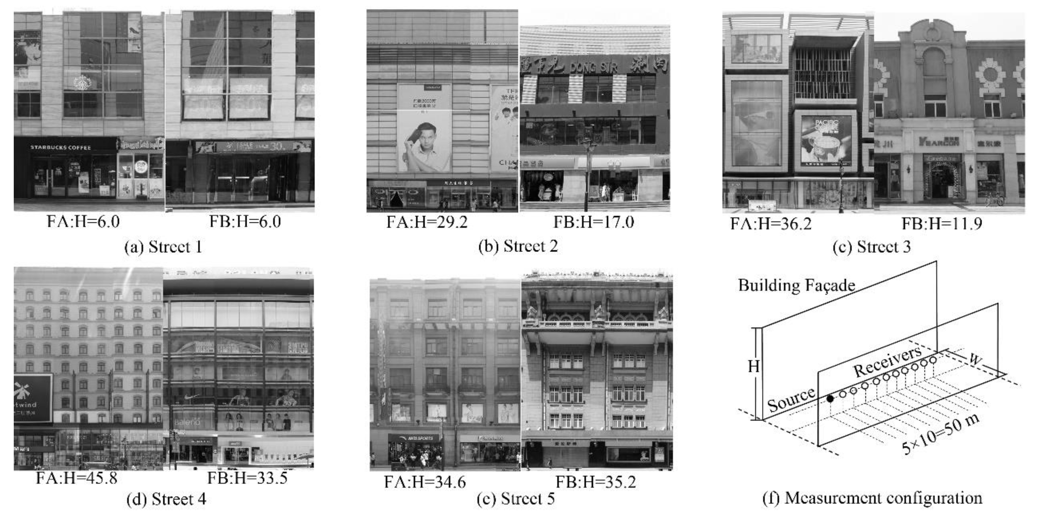
3.1. Site Selection for Full-Scale Measurement

To examine the accuracy of the IMCRI in an actual urban environment, full-scale measurements were carried out on five different streets (Figure 4a–e) in Tianjin, China. All five streets were straight streets with parallel building façades. The height of the building façades and the width of the streets were constant along the streets. Therefore, the geometry of the streets can be simplified as rectangles. Because the IMCRI mainly focused on the diffuse modeling scheme, the measured streets were selected so that the morphologies of the building façades in the five streets were quite different. As shown in Figure 4, various building façade conditions were found, which included very smooth cases (glass curtain walls on Street 1 and Street 4-FB), relatively rough cases (decorative structures on Street 3-FB), and very fluctuated cases (windows and balconies on Street 5 and rectangular structures on Street 3-FA). To control the sound absorption by building façades, the materials of building façades in all streets were similar and reflective and mainly made of glass and concrete. Moreover, there were no trees or wooden surfaces, which may lead to significant sound absorption.

All five streets were pedestrian shopping streets, and the measurements were carried out late at night (12:00–3:00 a.m.). The experimental zone was defined by the central 50 m of each street without a junction, while the length of each street was greater than 100 m. Therefore, the measurements were carried out when there were no pedestrians or vehicles nearby to avoid the direct influences of traffic noise.

3.2. Measurement System and Configuration

To conduct a full investigation of the sound field in a street, the sound attenuation and the sound decay were measured in this study. Different measurement systems were used to avoid the influence of background noise. Given the high signal-to-noise ratio requirement for the measurement of the reverberation time, a pistol source was employed in the RT measurements. A sound meter (Nor140, Norsonic, Lierskogen, Norway) was used to record the impulse response at each receiver position. While in the SPL measurements, an omnidirectional sound source with the pink signal was used to prevent the variations due to the pistol source. Meanwhile, in each receiver position, the SPL and impulse response were measured thrice to reduce the error caused by the background noise.

The main objective of the measurement in this study was to validate the calculation model in the streets with different diffuse conditions. Previous measurements revealed that sound attenuation along the length was more significant than that at the cross sections [30]. Therefore, the measurement configurations in the five streets were the same in this study, as shown in Figure 4f. The source was placed at the center of the street and 10 receivers were placed along the central axis at distances of 5 to 50 m from the source at intervals of 5 m. Because the most common source and receivers in the measured streets are the pedestrians, the height of the source and receivers were set at 1.25 m, as commonly used in previous measurements [38] and parameter studies [19]. During the measurements, the pistol, omnidirectional source, and sound meter were fixed to supports.

3.3. Estimation of Acoustic Parameters of Building Façades

The scattering coefficient for each building façade is needed to validate the calculation model. However, the measurement of the scattering coefficient of large building façades is difficult. The most common approach in previous studies is to use a hypothetical parameter that varies from 0 to 1 [13]. In this case, the comparison between simulations and measurements can only prove that the measured data is in the range of the simulation result instead of analyzing the detailed accuracy.

In this study, the laboratory-measured data from previous studies [39,40] were used to estimate the scattering coefficients of the actual building façades. A series of laboratory measurements focused on the scattering characteristics of the plate partially covered by geometric diffusers have been carried out, and the detailed scattering data of the samples with different shapes, sizes, and areas were reported [39,40,41,42]. It agreed with the result in reference [32] that the diffuse characteristics were mainly determined by the height (h) and the coverage density (CD) of the diffuse structures on the plate, as shown in Figure 5a. The frequency characteristics were mainly determined by the height of the structure. As shown in Figure 5a, in the laboratory experiment, the scattering coefficients increased in accordance with an increase in the frequency, and it reached a peak when h/λ (the height to the wavelength ratio) was approximately 0.1. When h/λ > 0.1, the curve was mainly constant with small fluctuations. Within the effective frequency range, the scattering coefficient was mainly determined by the coverage density, as shown in Figure 5b. With the increase in CD from 0, the scattering coefficient increased rapidly, and the growth rate gradually decreased. A decrease in the scattering coefficient was found when CD was very large (CD > 0.6). Therefore, the relationship between the coverage density and the scattering coefficient can be fitted as quadratic regression curves, as shown in Figure 5b. Three curves were established for three typical geometric diffusers respectively, including hemisphere (data from [39]), groove (data from [39]), and rectangular structures (data from [40]). As shown in Figure 5, the difference between these curves is fairly small (<0.2). Measured scattering coefficients of more complex structures [41] are also shown in Figure 5b, including a rectangular shape with flutters, a trapezoid shape, and triangular shape diffusers. As shown in Figure 5b, the scattering coefficients of these structures are close to those of the basic structures. They also agree with the result in Ref. [32] and indicates the feasibility of the estimated scattering coefficient of the actual building façade.

As shown in

Table 1. Coverage densities and estimated scattering coefficients of building façades on five measured streets. S_r, S_h, and S_g are the estimated scattering coefficients of the regression curves of groove, hemisphere, and rectangular diffusers, respectively.

Street Name	Coverage Density		Estimated Scattering Coefficient
	Façade A	Façade B	Façade A			Façade B
			Sr	Sh	Sg	Sr	Sh	Sg
Street 1	2.00%	7.00%	0.08	0.07	0.09	0.17	0.16	0.23
Street 2	6.50%	15.00%	0.16	0.15	0.22	0.30	0.28	0.42
Street 3	7.10%	10.60%	0.17	0.16	0.23	0.23	0.22	0.32
Street 4	35.00%	18.00%	0.52	0.52	0.71	0.34	0.33	0.48
Street 5	37.00%	54.00%	0.53	0.54	0.73	0.58	0.64	0.74

, by analyzing the morphology of the building façades, an overall coverage density of irregularities could be easily obtained, which could be further applied to the regression equations in Figure 5b to estimate the scattering coefficient. The estimated scattering coefficient in five measured streets varies from 0.07 to 0.74. The scattering coefficient of the actual building façade has been investigated in Ref. [13] by comparison between the simulation with the measurements. The scattering coefficient of build façades defined as a periodic arrangement of windows, which is very similar to Façade A of Street 4 in this study, is suggested to be 0.4–0.7. As shown in Table 1, the scattering coefficient of Façade A in Street 4 is estimated at 0.52–0.71, which is quite similar to the result in reference [13]. It should be noted that there are large structures in the actual building façade, i.e., sizable rectangles on Street 3-FA. When the dimensions of the plane surface are significantly larger than the wavelength, it functions similarly to a specular reflector rather than a diffuser [43]. Therefore, rectangular structures with large plane surfaces (the ratio of the dimension of the surface to the wavelength was larger than 10, 6.8 m for 500 Hz) were considered as planes rather than diffusers when counting the coverage density.

Given that the regression equation in Figure 5b was established by the data measured within the range of 0.1 < h/λ < 0.4, there was a frequency limitation of the estimated scattering coefficient. The common heights of diffuse structures in five measured streets varied from 10 to 15 cm. Therefore, the lower limit frequency for the estimated scattering coefficient was 227–340 Hz, which is approximately the lower limit frequency of the 500 Hz octave band. Meanwhile, the upper limit frequency was within the range of 900–1360 Hz, which is approximately the upper limit frequency of the 1000 Hz octave band. Therefore, in the model validation, the corresponding frequency range is analyzed (500 Hz and 1000 Hz octave bands).

In this study, building facades in the measured streets are all continuous surfaces with no junctions in the measurement zone. Therefore, the diffraction that needs to be considered is only caused by the irregular structures on the building façades. In fact, the multiple reflections and diffractions by these structures are the major causes of the scattering of the surfaces. The scattering coefficient in this study was estimated by the laboratory-measured data, which contained the influence of diffraction. Therefore, although no diffraction modeling process was applied in IMCRI, the influence of diffraction was considered by the scattering modeling process.

Another important acoustic parameter is the absorption coefficient, which may have an influence on the simulation results. As shown in Figure 4, all the building façades were made of glass and concrete, which can be considered as reflective materials in the frequency range of 500–1000 Hz. Measurements and estimations have been carried out for similar materials [38]. The absorption coefficient of the building façades varied from 0.03 to 0.09 in the range of 400–4000 Hz. Therefore, in the calculation model, the range of the absorption coefficient of the building façades was set as 0.05. Given that the ground surface in each measured street was very smooth and reflective, a scattering coefficient of 0.02 and an absorption coefficient of 0.02 were used. To simulate the atmosphere absorption, the temperature and humidity were also measured (Streets 1, 2, and 4: 10–12 °C, 75–80%; Streets 3 and 5: 3–7 °C, 72–85%). The air absorption was calculated using absorption attenuation coefficients with the measured temperature and relative humidity, in accordance with the ISO 9613-1.

4. Comparison between Calculation Models and Full-Scale Measurements

Based on the estimated coefficients, the accuracies of the IMCRI and existing models could be analyzed with full-scale measurement data. As shown in Table 1, the scattering coefficients estimated from rectangular structures (S_r) and hemisphere structures (S_h) are very similar, and are both smaller than the scattering coefficient estimated from the groove structures (S_g). Therefore, only S_r and S_g are shown in Figure 6 and Figure 7 to analyze the accuracy of IMCRI. Two existing models, the ISM and the ARM were also compared, which model the sound propagation process only by specular reflections and diffuse reflections, respectively. For SPL simulation, curves predicted by the Hopkins–Stryker equation are also shown as a reference.

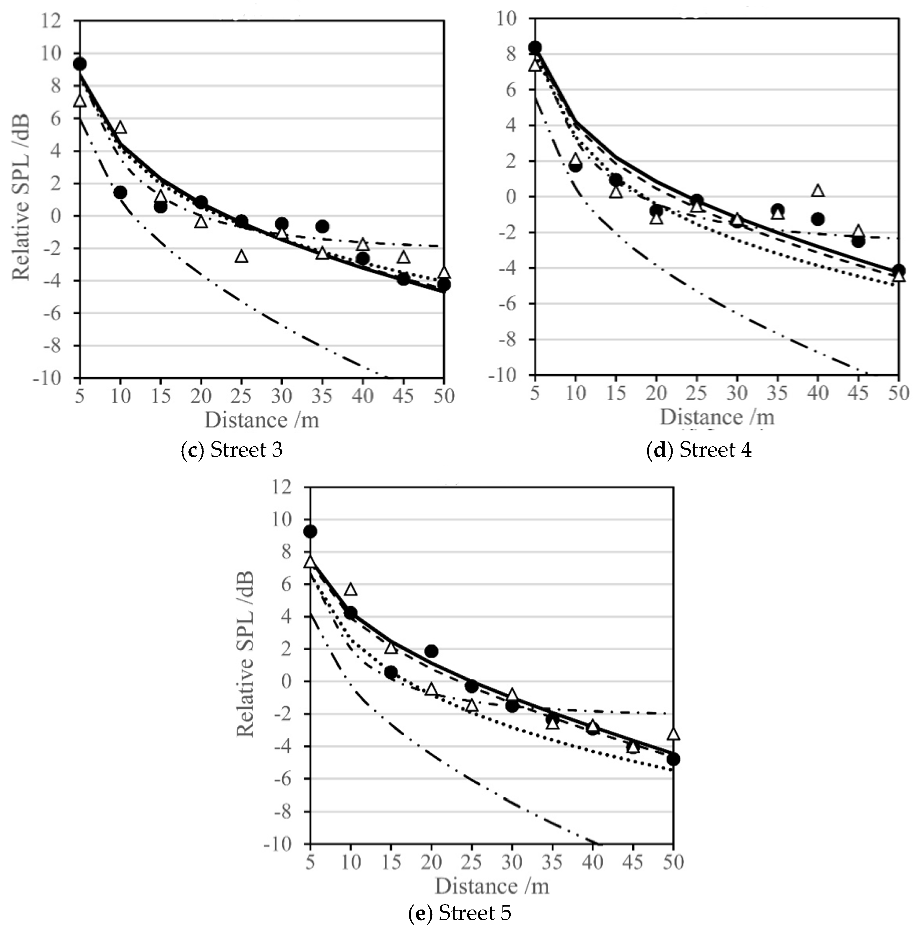
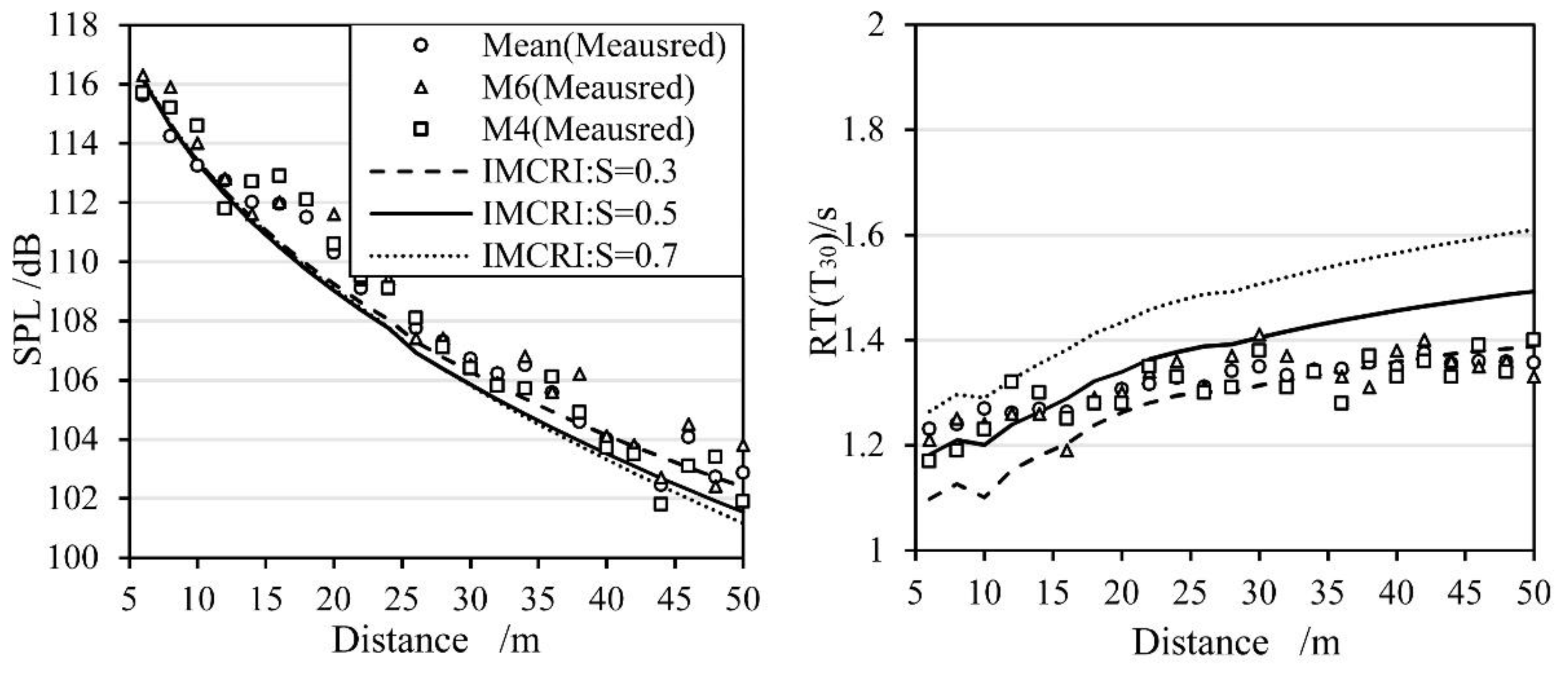
4.1. Sound Pressure Level along the Street

Figure 6 presents the results of the SPL attenuation along the street, where the ISM and IMCRI show good accuracies. In most receiver positions, the differences between these two models and measured data are smaller than 2 dB. Meanwhile, the ARM yields larger deviations, especially in streets with very smooth surfaces (Street 1). In the street with a smooth ground surface, the received sound energy is mainly determined by the direct sound and the first reflected sound from the ground. The late reflected sound energy, which is significantly influenced by the reflection modeling scheme, is only a small proportion of the overall sound energy. In ARM, the reflections on all surfaces are modeled as perfect diffuse reflections. However, this is very different from the situations on the actual façade, especially for the smooth ground surfaces. Meanwhile, in ISM, the ground surface is assumed to produce perfect specular reflection, which is relatively close to the real situation. In IMCRI, a small scattering coefficient (0.02) is assigned according to the scattering characteristics of the ground surface. Therefore, ISM and IMCRI achieve significantly higher accuracies than ARM in the SPL simulation. As expected, the error in the Hopkins–Stryker equation is significant when the façades are very smooth (Street 1 and Street 2, scattering coefficient <0.2). However, it shows relatively good performances in streets with fluctuated facades (Street 4 and Street 5), because the sound field is more diffuse in these streets.

Variations in the measured SPL attenuation are observed, as shown in Figure 6, especially in the far field (D > 25 m). These abnormal points only appear at a few positions in the specific frequency. Moreover, at a different frequency in the same position, the SPL attenuation curve is smooth. This indicates that the variations are probably due to accidental noise. Although the measurements were carried out late at night to achieve a relatively quiet environment, there were inevitable disturbances in the outdoor environment, i.e., wind sounds and accidental noises from surrounding areas. However, the differences among different models are much more significant than the variations. The performances of ISM and IMCRI are much better than that of ARM.

4.2. Reverberation Time along the Street

The mean absolute differences (MAD) between the measurements and simulations are calculated to analyze the model accuracy, as:

$$MAD=\frac{{{\displaystyle \sum }}_1^n\left|R{T}_{simulated,n}-R{T}_{measured,n}\right|}{n}.$$

(9)

Different from SPL, RT is mainly determined by the late reflected sound. Therefore, the reflection modeling scheme shows significant influences on RT simulations, which lead to different accuracies with these three calculation models. Figure 7 shows the RT comparison between calculation models and measurements, where IMCRI shows superior performance compared to the other two models. Good agreement between IMCRI and measured data are found in all five streets. With the estimated scattering coefficient, S_r, the MAD of IMCRI for all 50 receiver positions in five streets are 0.22 and 0.26 s for the 500 and 1000 Hz octave bands, respectively.

As shown in Figure 7, the accuracy of IMCRI varies in the five streets. In Street 1, Street 2, Street 4 and Street 5, the MADs of IMCRI with S_r are smaller than 0.2 s in the 500 and 1000 Hz octave bands. A relatively poor performance of IMCRI is found for Street 3, with a MAD larger than 0.6 s. It is probably caused by the overestimation of the scattering coefficient. As discussed in Section 3.3, all the laboratory-measured data in Figure 5b used to estimate the scattering coefficient in the actual streets were measured using limited implementations: 0.1 < h/λ < 0.4. However, in Street 3, diffuse structures with depths greater than 1 m can be found, which results in a significantly larger h/λ in the considered frequency range. As reported by previous studies, the scattering coefficient decreases with the increase of h/λ when h/λ is large [41]. With the scattering coefficient of 0.3 S_r, good agreement between IMCRI and measurements can be achieved (MAD < 0.2). Supplementary measurements of the scattering coefficient with a larger range of h/λ can be carried out to solve the problem. The depth of measured structures in Figure 5 varies from 1.5 to 4.7 cm. In reference [41], the scattering coefficients of structures with a depth of 8 cm was measured within the frequency range of 100 to 5000 Hz. With such implementations, the scattering coefficient when h/λ > 1 can be investigated.

Although the performances of IMCRI with S_g and S_r are similar, IMCRI with S_r is more accurate than IMCRI with S_g in most measured streets. In Street 1, Street 2 and Street 3, the MADs of IMCRI with S_g are approximately 0.2 to 0.4 s larger than that of IMCRI with Sr. The possible reason for this phenomenon is that S_r is more similar to the scattering characteristic of the actual building façades, because the shape of the structures attached to the building façades is relatively similar to that of rectangular structures, as shown in Figure 4. As reported by previous studies, the influence of the scattering coefficient is relatively small when the scattering coefficient is large [17,19]. In Street 4 and Street 5, the estimated scattering coefficients are between 0.5 and 0.7, while the difference between S_g and S_r is approximately 0.15. Therefore, the IMCRI with different scattering coefficients shows very similar results in these streets.

4.3. Comparison between Iterative Model Combining the Radiosity Method and Image Source Method (IMCRI) and the Existing Hybrid Model of Image Source Model (ISM) and Acoustic Radiosity Model (ARM)

An existing hybrid model (EHM) of ISM and ARM was developed to reveal the improvement by modeling image patches (specular reflections after diffuse reflections) in the IMCRI. The difference in the reflection modeling scheme between the IMCRI and EHM is described in Section 2. Other implementations in the EHM were the same as the IMCRI.

Figure 8 shows the comparison between the IMCRI and EHM (SPL_IMCRI-SPL_EHM and RT_IMCRI-RT_EHM) with different building façade heights and scattering coefficients. As shown in Figure 8a, the differences between IMCRI and EHM were small (<1.5 dB and 0.3 s) in the street with low building façades (H = 5). However, in the street with high building façades (H = 45), significant differences of up to 5.5 dB and 1.7 s were found, as shown in Figure 8b.

Because the modeling scheme mainly affects the high-order reflected sound, the SPL difference between IMCRI and EHM varied with the distance from the source. No significant differences were found in the near-field (D = 5) in both streets because it was dominated by the direct sound and the specular reflected sound of the ground. However, there were considerable differences in the far-field (D = 50) when the scattering coefficient increased. The maximum difference was approximately 1.5 and 5.5 dB in two streets with different building façade height. On the contrary, the RT difference between IMCRI and EHM was independent of the distance because it was mainly determined by the late reflected sound. The RT difference between EHM and IMCRI was significantly larger in streets with high building façades.

In general, this result shows that the reflection modeling scheme has significant influences on SPL and RT simulations in streets with high building façades, which is common in modern cities. By considering the full sound energy transfer path, the IMCRI can significantly improve the simulation accuracy of SPL in the far-field and RT in the whole street.

Because more sound transfer paths were calculated in the IMCRI, the time cost of the IMCRI was larger than EHM in most cases, as shown in

Table 2. The time cost of existing hybrid model (EHM) and the IMCRI. W, H, and S are street width, building façade height and the scattering coefficient of the building façade, respectively.

Time Cost/s	Street 1: W = 15; H = 6			Street 6: W = 16; H = 35
	S = 0.05	S = 0.5	S = 0.95	S = 0.05	S = 0.5	S = 0.95
EHM	53	97	102	1827	2258	2576
IMCRI	44	96	153	5016	15891	14491
Ratio (IMCRI/EHM)	0.8	1.0	1.5	2.7	7.0	5.6

. As described in Section 2, an auto-termination process was used in the IMCRI to decide whether a sufficient number of paths were calculated and to stop the whole calculation process. In the street with high building façades (W = 16; H= 35), more iterations were needed due to the strong influence of scattering sound energy from the building façades. In this case, the IMCRI required a calculation time that was greater than that of the EHM by an approximate factor of 2.5–7. In streets with a low, flat building façade (W = 15; H = 6), only a small part of the sound energy was scattered by the building façade. The termination condition could be achieved with a few iterations. Therefore, the time cost of the IMCRI was similar to that of the EHM and was even less when the scattering coefficient was very low. The results in Figure 8 and Table 2 show that a good balance between model accuracy and time cost was achieved by the auto-determination process in the IMCRI.

5. Discussion

In this study, a hybrid model combining ISM and ARM is proposed. By contrast with the existing hybrid models, the full sound transfer paths can be considered in the IMCRI. The comparison between EHM and the IMCRI shows that the accuracy of EHM is relatively acceptable when the building façade is very low. However, streets with high-rise buildings are more common in modern urban areas, where the IMCRI shows superior performance. Meanwhile, the IMCRI is also shown to be highly efficient with regard to time due to the application of the auto-termination process, which is crucial for simulating sound propagation in large urban areas. The most time-consuming task in the IMCRI is the calculation of the form factor between patches. However, it is independent of the source and receivers, and pre-calculated before the sound energy transfer process. Therefore, the time efficiency of the IMCRI can be further improved.

Measurements in five streets are used to validate the IMCRI in this study. Another full-scale measurement in a French street [30] has been widely used to investigate the performance of calculation models [13,15]. In this measurement, the SPL and RT were measured using multiple sound sources and receiver positions. Figure 9 shows the comparison between the IMCRI and this measurement. As described in reference [30], the morphology of the building façade in this street was defined as a periodic arrangement of windows. Due to the lack of detailed information on façade morphology, a relatively wide range of scattering coefficients (0.3–0.7) is applied to evaluate the behavior of the IMCRI. As shown in Figure 9, the IMCRI and measured data are in good agreement. The IMCRI with a relatively low scattering coefficient (0.3) shows the best performance.

It should be noted that there are some limitations in the IMCRI. First, modeling the surface details is difficult in the IMCRI, although it is reported to be a benefit as it improves the accuracy of GA models [44]. Due to the scheme of radiosity model, the calculation of the form factor between patches can be very complicated and time-consuming, when the shape of the patch is irregular. Meanwhile, estimating the scattering coefficient for small surfaces is more difficult than the large surfaces because of the difficulties in estimating the edge effect. Therefore, the detailed modeling of surfaces in the IMCRI will lead to a significant increase in the time cost and uncertain influences on the model accuracy. Second, the IMCRI is a pure energy-based model where no phase information is considered. In this study, it has been proven to be accurate in relatively wide streets (15 to 25 m wide) and the middle-frequency range (500 and 1000 Hz octave bands). However, phase information might be crucial in narrow streets [45] and a low-frequency range [46].

6. Conclusions

An iterative model that combined the radiosity method and image source method (IMCRI) was developed in this study, which considers both the specular and diffuse components for each reflection. Full-scale measurements of five urban streets were carried out to validate the calculation model. Good agreement between measurements and simulations using IMCRI is found, which indicates good accuracy and extensive applicability. The performance of the IMCRI is superior to that of the existing models, especially for the RT simulation. By comparing the IMCRI with existing hybrid models, it is found that the modeling of full sound transfer paths leads to considerable improvements, especially in streets with high and irregular building façades.

In the future, we will focus on how to merge phase information into the IMCRI, which is necessary for investigating the effect of scattering in narrow streets and at a low-frequency range. Furthermore, it can also be used to investigate sound propagation in more complex situations, for instance, shielded space and streets with branches.

References

1. Lee, P.J.; Jeon, J.Y. Evaluation of speech transmission in open public spaces affected by combined noises. J. Acoust. Soc. Am. 2011, 130, 219. [Google Scholar] [CrossRef] [PubMed]
2. Miedema, H.M.; Oudshoorn, C.G. Annoyance from transportation noise: Relationships with exposure metrics DNL and DENL and their confidence intervals. Environ. Health Perspect. 2001, 109, 409–416. [Google Scholar] [CrossRef] [PubMed]
3. Morihara, T.; Sato, T.; Yano, T. Comparison of dose–response relationships between railway and road traffic noises: The moderating effect of distance. J. Sound Vib. 2004, 277, 559–565. [Google Scholar] [CrossRef]
4. Muzet, A. Environmental noise, sleep and health. Sleep Med. Rev. 2007, 11, 135–142. [Google Scholar] [CrossRef] [PubMed]
5. Babisch, W.; Beule, B.; Schust, M.; Kersten, N.; Ising, H. Traffic Noise and Risk of Myocardial Infarction. Epidemiology 2005, 16, 33–40. [Google Scholar] [CrossRef] [PubMed]
6. Van Kempen, E.; Babisch, W. The quantitative relationship between road traffic noise and hypertension: A meta-analysis. J. Hypertens. 2012, 30, 1075–1086. [Google Scholar] [CrossRef]
7. Hui, M.; Shan, S. An Experimental Study: The Restorative Effect of Soundscape Elements in a Simulated Open-Plan Office. Acta Acust. United Ac. 2018, 104, 106–115. [Google Scholar]
8. Davis, M.J.M.; Tenpierik, M.J.; Ramírez, F.R.; Pérez, M.E. More than just a Green Facade: The sound absorption properties of a vertical garden with and without plants. Build. Environ. 2017, 116, 64–72. [Google Scholar] [CrossRef]
9. Van Renterghem, T.; Botteldooren, D. In-situ measurements of sound propagating over extensive green roofs. Build. Environ. 2011, 46, 729–738. [Google Scholar] [CrossRef] [Green Version]
10. Guillaume, G.; Gauvreau, B.; Hermite, P.L. Numerical study of the impact of vegetation coverings on sound levels and time decays in a canyon street model. Sci. Total Environ. 2015, 502, 22–30. [Google Scholar] [CrossRef]
11. Van Renterghem, T.; Salomons, E.; Botteldooren, D. Parameter study of sound propagation between city canyons with a coupled FDTD-PE model. Appl. Acoust. 2006, 67, 487–510. [Google Scholar] [CrossRef] [Green Version]
12. Echevarria Sanchez, G.M.; Van Renterghem, T.; Thomas, P.; Botteldooren, D. The effect of street canyon design on traffic noise exposure along roads. Build. Environ. 2016, 97, 96–110. [Google Scholar] [CrossRef] [Green Version]
13. Le Pollès, T.; Picaut, J.; Bérengier, M.; Bardos, C. Sound field modeling in a street canyon with partially diffusely reflecting boundaries by the transport theory. J. Acoust. Soc. Am. 2004, 116, 2969–2983. [Google Scholar] [CrossRef]
14. Badino, E.; Manca, R.; Shtrepi, L.; Calleri, C.; Astolfi, A. Effect of façade shape and acoustic cladding on reduction of leisure noise levels in a street canyon. Build. Environ. 2019, 157, 242–256. [Google Scholar] [CrossRef]
15. Lee, P.J.; Kang, J. Effect of height-to-width ratio on the sound propagation in urban streets. Acta Acust. United Ac. 2015, 101, 73–87. [Google Scholar] [CrossRef]
16. Radwan, M.M.; Oldham, D.J. The prediction of noise from urban traffic under interrupted flow conditions. Appl. Acoust. 1987, 21, 163–185. [Google Scholar] [CrossRef]
17. Can, A.; Fortin, N.; Picaut, J. Accounting for the effect of diffuse reflections and fittings within street canyons, on the sound propagation predicted by ray tracing codes. Appl. Acoust. 2015, 96, 83–93. [Google Scholar] [CrossRef]
18. Kang, J. Sound propagation in street canyons: Comparison between diffusely and geometrically reflecting boundaries. J. Acoust. Soc. Am. 2000, 107, 1394–1404. [Google Scholar] [CrossRef]
19. Onaga, H.; Rindel, J.H. Acoustic characteristics of urban streets in relation to scattering caused by building facades. Appl. Acoust. 2007, 68, 310–325. [Google Scholar] [CrossRef]
20. Meng, Y.; Kang, J. Combined Ray-tracing and Radiosity Simulation for Urban Open Spaces. In Proceedings of the 19th International Congress on Acoustics, Madrid, Spain, 2–7 September 2007; pp. 2–7. [Google Scholar]
21. Lyon, R.H. Role of multiple reflections and reverberation in urban noise propagation. J. Acoust. Soc. Am. 1974, 55, 493–503. [Google Scholar] [CrossRef]
22. Schröder, D.; Pohl, A. Modeling (Non-)uniform scattering distributions in geometrical acoustics. In Proceedings of the Meetings on Acoustics, Montreal, QC, Canada, 2–7 June 2013; pp. 1–9. [Google Scholar]
23. Howell, J.R.; Siegel, R.; Mengüç, M.P. Thermal radiation heat transfer, 2nd ed.; Hemisphere: Washington, DC, USA, 1981. [Google Scholar]
24. Kang, J. Numerical modelling of the sound fields in urban streets with diffusely reflecting boundaries. J. Sound Vib. 2002, 258, 793–813. [Google Scholar] [CrossRef]
25. Korany, N.; Blauert, J.; Alim, O.A. Acoustic simulation of rooms with boundaries of partially specular reflectivity. Appl. Acoust. 2001, 62, 875–887. [Google Scholar] [CrossRef]
26. Ismail, M.R.; Oldham, D.J. A scale model investigation of sound reflection from building façades. Appl. Acoust. 2005, 66, 123–147. [Google Scholar] [CrossRef]
27. Wiener, F.M.; Malme, C.I.; Gogos, C.M. Sound propagation in urban areas. J. Acoust. Soc. Am. 1965, 37, 738. [Google Scholar] [CrossRef]
28. Yeow, K.W. External reverberation times observed in built-up areas. J. Sound Vib. 1976, 48, 438–440. [Google Scholar] [CrossRef]
29. Yeow, K.W. Decay of sound levels with distance from a steady source observed in a built-up area. J. Sound Vib. 1977, 52, 151–154. [Google Scholar] [CrossRef]
30. Picaut, J.; Le Pollès, T.; L’Hermite, P.; Gary, V. Experimental study of sound propagation in a street. Appl. Acoust. 2005, 66, 149–173. [Google Scholar] [CrossRef]
31. Horoshenkov, V.; Hothersall, C.; Mercy, E. Scale modelling of sound propagation in a city street canyon. J. Sound Vib. 1999, 223, 795–819. [Google Scholar] [CrossRef]
32. Picaut, J.; Simon, L. A scale model experiment for the study of sound propagation in urban areas. Appl. Acoust. 2001, 62, 327–340. [Google Scholar] [CrossRef]
33. Hornikx, M.; Forssén, J. A scale model study of parallel urban canyons. Acta Acust. United Ac. 2008, 94, 265–281. [Google Scholar] [CrossRef]
34. Tang, S.K.; Piippo, K.E. Sound fields inside street canyons with inclined flanking building facades. In Proceedings of the 161st Meeting Acoustical Society of America 2011, Seattle, WA, USA, 23–27 May 2011; Acoustical Society of America: Seattle, WA, USA, 2011; Volume 12, pp. 1–7. [Google Scholar]
35. Jang, H.S.; Lee, S.C.; Jeon, J.Y.; Kang, J. Evaluation of road traffic noise abatement by vegetation treatment in a 1:10 urban scale model. J. Acoust. Soc. Am. 2015, 138, 3884–3895. [Google Scholar] [CrossRef] [PubMed]
36. Jang, H.S.; Kim, H.J.; Jeon, J.Y. Scale-model method for measuring noise reduction in residential buildings by vegetation. Build. Environ. 2015, 86, 81–88. [Google Scholar] [CrossRef]
37. Le Pollès, T.; Picaut, J.; Colle, S.; Bérengier, M.; Bardos, C. Sound-field modeling in architectural acoustics by a transport theory: Application to street canyons. Phys. Rev. E 2005, 72, 1–17. [Google Scholar] [CrossRef] [PubMed]
38. Li, K.M.; Lai, C.Y.C. A note on noise propagation in street canyons. J. Acoust. Soc. Am. 2009, 126, 644–655. [Google Scholar] [CrossRef] [PubMed]
39. Kim, Y.H.; Jang, H.S.; Jeon, J.Y. Characterizing diffusive surfaces using scattering and diffusion coefficients. Appl. Acoust. 2011, 72, 899–905. [Google Scholar] [CrossRef]
40. Schmich-Yamane, I.; Embrechts, J.-J.; Muller-Trapet, M.; Rougier, C.; Malgrange, M.; Vorlander, M. Prediction and measurement of the random-incidence scattering coefficient of periodic reflective rectangular diffuser profiles. In Proceedings of the International Congress on Acoustics, Montreal, QC, Canada, 2–7 June 2013; Acoustical Society of America: Montreal, QC, Canada, 2013; Volume 19, pp. 1–9. [Google Scholar]
41. Lin, F.; Hong, P.; Lee, C. An experimental investigation into the sound-scattering performance of wooden diffusers with different structures. Appl. Acoust. 2010, 71, 68–78. [Google Scholar] [CrossRef]
42. Yong, J.; Chan, S.; Vorla, M. Development of scattering surfaces for concert halls. Appl. Acoust. 2004, 65, 341–355. [Google Scholar] [CrossRef]
43. Embrechts, J.J.; Billon, A. Theoretical Determination of the Random-Incidence Scattering Coefficients of Infinite Rigid Surfaces with a Periodic Rectangular Roughness Profile. Acta Acust. United Ac. 2011, 97, 607–617. [Google Scholar] [CrossRef]
44. Shtrepi, L. Investigation on the diffusive surface modeling detail in geometrical acoustics based simulations. J. Acoust. Soc. Am. 2019, 145, EL215–EL221. [Google Scholar] [CrossRef] [Green Version]
45. Iu, K.K.; Li, K.M. The propagation of sound in narrow street canyons. J. Acoust. Soc. Am. 2002, 112, 537–550. [Google Scholar] [CrossRef]
46. Richoux, O.; Ayrault, C.; Pelat, a.; Félix, S.; Lihoreau, B. Effect of the open roof on low frequency acoustic propagation in street canyons. Appl. Acoust. 2010, 71, 731–738. [Google Scholar] [CrossRef] [Green Version]
Figure 1. Schematic diagram of (a) iterative model combining the radiosity method and image source method (IMCRI); (b) existing hybrid models (EHM) and (c) sound energy transfer paths. D and S represent the specular reflected energy and the diffuse reflected energy. The red line and blue line represent the components calculated by image source model (ISM) and acoustic radiosity model (ARM) in EHM, respectively.
Applsci 09 02803 g001
Figure 2. Sound energy transfer from sources to patches. In the figure above, d and θ represent the distance and the incident angle from the source to the patch, respectively.
Applsci 09 02803 g002
Figure 3. Effect of termination threshold on simulation results. D is the distance from the source.
Applsci 09 02803 g003
Figure 4. Images of measured street canyons (ae) and measurement configuration (f).
Applsci 09 02803 g004
Figure 5. Effect of size, coverage density, and structure type on the scattering coefficients: (a) scattering coefficients of samples with different heights; (b) relationship between the coverage density and scattering coefficient for different structures (0.1 < h/λ < 0.4). The solid line, dotted line, and dash–dot line are quadratic regression curves for groove, hemisphere and rectangular diffusers, respectively.
Applsci 09 02803 g005
Figure 6. Predicted and measured sound pressure level (SPL) attenuation of the five actual street canyons. S is the scattering coefficient of the building façade. (a)–(e) are results in Streets 1–5.
Applsci 09 02803 g006aApplsci 09 02803 g006b
Figure 7. Predicted and measured reverberation time (RT) (T30) of the five actual street canyons. S is the scattering coefficient of the building façade. MAD is the mean absolute differences between the measurements and IMCRI.
Applsci 09 02803 g007
Figure 8. The comparison between the IMCRI and EHM in two streets. D, W, H, and S are the distance from the source, street width, building façade height, and the scattering coefficient of the building façade, respectively.
Applsci 09 02803 g008aApplsci 09 02803 g008b
Figure 9. Comparison between the IMCRI and measurements in a French street. M4, M6, and Mean represent the receiver positions close to the building façades, along the central axis, and the mean values of all nine receiver positions, respectively. S is the scattering coefficient of the building façade.
Applsci 09 02803 g009