Numerical Investigation of Jet Angle Effect on Airfoil Stall Control

Abstract

Numerical study on flow separation control is conducted for a stalled airfoil with steady-blowing jet. Stall conditions relevant to a rotorcraft are of interest here. Both static and dynamic stalls are simulated with solving compressible Reynolds-averaged Navier-Stokes equations. It is expected that a jet flow, if it is applied properly, provides additional momentum in the boundary layer which is susceptible to flow separation at high angles of attack. The jet angle can influence on the augmentation of the flow momentum in the boundary layer which helps to delay or suppress the stall. Two distinct jet angles are selected to investigate the impact of the jet angle on the control authority. A tangential jet with a shallow jet angle to the surface is able to provide the additional momentum to the flow, whereas a chord-normal jet with a large jet angle simply averts the external flow. The tangential jet reduces the shape factor of the boundary layer, lowering the susceptibility to the flow separation and delaying both the static and dynamic stalls.

1. Introduction

Stall occurs when a lifting surface loses its aerodynamic lift. A well-known reason of the stall is the flow separation from the surface. An airfoil would be the best example to describe the stall phenomenon. As the angle of attack $\alpha$ increases beyond the stall angle ${\alpha }_{stall}$, the flow is detached from the airfoil surface. The flow may separate from the trailing edge or the leading edge, depending on the specific design of an airfoil and the flow condition including the Reynolds and Mach numbers [1].

The stall phenomenon associated with a lifting body at fixed angles of attack is called static stall. In contrast to static stall, dynamic stall occurs when the angle of attack changes rapidly due to airfoil motion. In this study, both static and dynamic stall are investigated. For dynamic stall, a pitching motion is assigned to an airfoil with the maximum pitch angle being significantly larger than the static stall angle.

Static and dynamic stall of an airfoil are depicted in Figure 1. Several key stages of the dynamic stall are compared to the static stall for the OA209 airfoil at the Mach number $Ma=0.3$ and the Reynolds number $Re=\frac{\rho U_{\infty }c}{\mu }=1.15\times {10}^6$ where $\rho$ is the density, $U_{\infty }$ is the freestream velocity, c is the airfoil chord length, and $\mu$ is the viscosity. The non-dimensionalized pitching frequency $k=2\pi fc/\left(2U_{\infty }\right)$ is determined for a rotor-relevant pitch frequency. Stage 1 in the upstroke region, which is still before the static stall angle, is similar to the static airfoil. Around stage 2, dynamic stall vortex (DSV) is formed near the leading edge. DSV reduces the pressure on the suction side further, compared to the static case, which results in the lift increase. From stage 2 to 3, DSV convects downstream, inducing more lift. Such additional lift is accompanied with the drag increase. From stage 2 to 3, the moment stall occurs as DSV moves to the trailing edge. The moment stall indicates a significant pitching-down moment because of the additional lift near the trailing edge. From stage 3 to 4, DSV is finally detached from the surface, which results in the lift stall. At stage 5, near the peak angle, shedding vortices produce the load fluctuation. In the downstroke region, the airfoil undergoes the severe stall until a small enough angle for the flow to reattach on the airfoil from the leading edge, which occurs around stage 6. The cycle restarts, as the angle reaches to the minimum.

Stall phenomena, typically dynamic stall, impact on designing and analyzing lift surfaces. For example, conventional helicopter main rotor blades frequently encounter dynamic stall in high-speed forward flight conditions [2,3,4,5,6,7]. The blade stall can occur in the retreating side because the blade needs to pitch up in order to balance aerodynamic forces. The retreating blade stall can decrease the performance of the helicopter and cause structural damage in the main rotor system. In contrast to the rotary wing, fixed-wing aircraft can use dynamic stall to improve performance such as super-maneuverability [8,9,10]. Wind turbine blades also experience dynamic stall under highly unsteady conditions [11,12,13,14].

Stall suppression with an active flow control technique is of interest in this study. Various active flow control techniques using fluidic actuators have been studied to mitigate flow separation [15,16,17,18,19,20,21,22,23,24,25,26,27,28,29]. Among numerous methods, steady-blowing jet would be the simplest fluidic actuation, ejecting a jet flow continuously into the surrounding. Recently, Gardner et al. investigated steady-blowing jet of high jet momentum in both simulation and wind tunnel tests [16,17,18,19]. Their experiments demonstrate that the steady-blowing jet which is normal to the airfoil chord is able to suppress the moment stall. It, however, comes at a price of non-negligible reduction in the aerodynamic lift. Furthermore, the effect of the jet angle on the flow control was not separated from other jet parameters including the jet location and the jet size. It seems that the effect of the jet angle on the flow control performance needs to be investigated systemically. Compared to the high jet angle of the chord-normal jet, a shallow angle would allow the jet to reside in the boundary layer longer and to energize the flow more, which helps to delay the stall and improve the aerodynamic performance of a lifting body.

The flow control performance of a jet flow is primarily determined by three major parameters: the jet location $x_{jet}$, the jet angle ${\theta }_{jet}$ and the jet momentum, normally given by the jet momentum coefficient $c_{\mu }=\frac{{\dot{m}}_{jet}{v}_{jet}}{{\rho }_{\infty }{U}_{\infty }^{2}bc}$ where ${\dot{m}}_{jet}$ is the mass flow rate of the jet, $v_{jet}$ is the jet velocity, and b is the span length of a wing. Based on previous studies with steady-blowing jet [16,19,20,30] and oscillatory jets [31], an upstream jet location near the leading edge $x/c\simeq 0.1$ outperforms downstream locations. Flow control studies with pulsed jets [21,22,23] also indicate that positions near the leading edge $0.05\le x_{jet}/c\le 0.15$ are able to mitigate the flow separation further when compared to a slightly downstream location of $x/c=0.2$.

A significant jet momentum is required to achieve meaningful control authority over the separation boundary layer [15]. Poisson-Quinton and Lepage [32] and Attinello [33] presented that the steady-blowing jet can be detrimental, if the momentum coefficient $c_{\mu }$ is “low”, i.e., $c_{\mu }\lesssim 0.01$. A large jet momentum up to $c_{\mu }\approx 0.05$ can improve the performance of a lifting body, increasing both the lift coefficient $c_l$ and the rate $d{c}_l/d{c}_{\mu }$. Thus many studies of jet blowing (steady or unsteady) for flow control have been conducted with the jet momentum in the order of the magnitude of $c_{\mu }=\mathcal{O}\left(0.01\right)$ [16,17,18,19,21,22,23]. A concise review of the blowing parameter can be found in [34,35]. Following the experiments [16,17,18], the jet momentum coefficient $c_{\mu }=0.06$ is used in this study, satisfying the earlier founding of the minimum requirement for the jet momentum.

In contrast to the jet location and the jet momentum, the impact of the jet angle on the separation control has not been systematically investigated in the literature. Recent studies on steady-blowing jet [16,17,18,19] primarily focus on a large jet angle ${\theta }_{jet}$ with respect to the wing surface. Although a small jet angle was also used in the computations of [19], other jet parameters including the jet location were also varied at the same time. It was not straightforward to distinguish the effect of the jet angle on the stall control from other jet parameters. Therefore, in the current study, of the primary interest is the effect of the jet angle on the dynamic stall.

The hypothesis in this study is that a jet ejected at a shallow angle toward the airfoil surface can add the jet momentum more to the boundary layer, compared to a larger jet angle. Two distinct jet angles are selected to test this hypothesis. A small enough angle is determined for a tangential jet which ejects almost tangentially to the airfoil surface. A large jet angle normal to the chord line is used for a chord-normal jet. Those two angles are ${\theta }_{jet}=22°$ and 80° in this study. The shallow angle ${\theta }_{jet}=22°$ is suggested for a practical limit for the fabrication of a jet actuator in Matalanis et al. [21,22].

Computational methods are followed in Section 2. In Section 3, computational results of the nominal airfoil are compared to relevant literature data [19,36,37,38]. Then, stall control with the variation of the jet angle is investigated for both the static and dynamic stalls. Conclusions are followed in Section 4.

2. Methods

2.1. Flow Conditions

The OA209 airfoil under the freestream condition of the Mach number $Ma=0.3$ and the Reynolds number $Re=1.15\times {10}^6$ is simulated here, following the experimental conditions [16,17,36]. The static pressure and the static temperature in the freestream are $P_{\infty }=56$ kPa and $T_{\infty }=304$ K, respectively. The freestream velocity is $U_{\infty }=105$ m/s.

The airfoil pitches about the quarter-chord point with a pitching motion prescribed in Equation (1).

$$\alpha ={\alpha }_0+{\alpha }_{1}sin\left(2\pi ft\right)$$

(1)

where $\alpha$ is the angle of attack, ${\alpha }_0$ is the mean angle of attack, ${\alpha }_1$ is the amplitude of the sinusoidal motion, t is the time and f is the pitching frequency. The pitching frequency f is non-dimensionalized to the reduced frequency k using Equation (2)

$$k=\frac{2\pi fc}{2U_{\infty }}$$

(2)

For deep dynamic stall in this study, a pitching motion of $\alpha =13°+7°sin\left(2\pi ft\right)$ is assigned with the reduced frequency $k=0.05$, following the experimental condition of [38]. The chord length of the airfoil is $c=0.3$ m.

Two jet angles are selected in the current study: ${\theta }_{jet}=80°$ for the chord-normal jet and ${\theta }_{jet}=22°$ for the tangential jet. The jet outlet is located at $x_{jet}/c=0.1$ on the suction side, following the test [16,17]. The wind tunnel test of Gardner et al. [17] was conducted with round holes discretely positioned in the span, which is not appropriate in the current 2D simulation. As a consequence, a fully spanned jet is modeled with the same jet momentum $c_{\mu }=0.06$ of [16,17]. To match the jet momentum to the counterpart from one round hole of the diameter d per the wing span b of [16,17], the jet width $w_{jet}/c=0.001$ is determined from the relation $c_{\mu }=\frac{{\rho }_{jet}{v}_{jet}^2{w}_{jet}}{{\rho }_{\infty }{U}_{\infty }^{2}c}=\frac{{\rho }_{jet}{v}_{jet}^2\frac{\pi }{4}{w_{jet}}^2}{{\rho }_{\infty }{U}_{\infty }^{2}cb}$. The total pressure $P_t=290$ kPa and the total temperature $T_t=300$ K are used for the total condition of the jet actuation.

2.2. Numerical Methods

The compressible Reynolds-averaged Navier-Stokes (RANS) equations are computed numerically using the unstructured flow solver SU2, which was developed in Stanford university [39]. The RANS equations are obtained using the Favre average. Here, the Favre average is given by $\tilde{\varphi }=\frac{\overline{\rho \varphi }}{\overline{\rho }}$ where $\varphi$ is an instantaneous variable and the overbar indicates the conventional Reynolds-averaged $\varphi$. The compressible RANS equations are given by

$$\frac{\partial \overline{\rho }}{\partial t}+\frac{\partial }{\partial x_i}\left(\overline{\rho }\widetilde{u_i}\right)=0$$

(3)

$$\frac{\partial }{\partial t}\left(\overline{\rho }\widetilde{u_i}\right)+\frac{\partial }{\partial x_j}\left(\overline{\rho }\widetilde{u_i}\widetilde{u_j}\right)+\frac{\partial }{\partial x_j}[\overline{p}{\delta }_{ij}-{\tau }_{ij}^{turb}]=0$$

(4)

$$C_v\frac{\partial }{\partial t}\left(\overline{\rho }\tilde{T}\right)+\frac{\partial }{\partial x_j}[\left(C_v\overline{\rho }\widetilde{u_j}\tilde{T}\right)+\overline{p}\widetilde{u_j}+\widetilde{u_i}\widetilde{{\tau }_{turb}}-\lambda \tilde{T}+C_v{q}_j^{turb}]=0$$

(5)

where ${\tau }_{ij}^{turb}=2{\mu }_t\widetilde{S_{ij}^{*}}-\frac{2}{3}\overline{\rho }k{\delta }_{ij}$. The equation of state for a calorically perfect gas is used here. Unless notified otherwise, the following scales are used for non-dimensionalization: $U_{\infty },c,P_{\infty },T_{\infty }$ and ${\rho }_{\infty }$.

The standard Spalart-Allmaras (SA) model is used to model the turbulent viscosity ${\mu }_t$ [40]. The SA model is given by

$$\frac{D\widehat{\nu }}{Dt}=c_{b1}\tilde{S}\widehat{\nu }+\frac{1}{\sigma }[\nabla ((\nu +\widehat{\nu })\nabla \widehat{\nu }+c_{b2}{(\nabla \widehat{\nu })}^2]-\left[c_{w1}{f}_w\right]{\left[\frac{\widehat{\nu }}{d}\right]}^2$$

(6)

where ${\nu }_t$ is defined as ${\nu }_t=\frac{{\mu }_t}{\rho }=\widehat{\nu }{f}_{v1}$. The working variable $\widehat{\nu }$ is obtained from the SA transport Equation (6). In addition, the following model coefficients are used: $c_{b1}=0.1355,c_{b2}=0.622,\kappa =0.41,\sigma =\frac{2}{3},c_{w1}=\frac{c_{b1}}{{\kappa }^2}+\frac{1+c_{b2}}{\sigma },c_{w2}=0.3,c_{w3}=2,c_{v1}=7.1$. The turbulent heat flux $q_j^{turb}$ is modeled using the temperature gradient $q_j^{turb}\equiv C_p\frac{{\mu }_t}{P{r}_t}\frac{\partial \tilde{T}}{\partial x_j}$ where the turbulent Prandtl number is $P{r}_t=0.9$ and the heat capacity at constant pressure $C_p$ for the air is used. The numerical analysis is conducted with the assumption of fully turbulent flow. It should be noted that typical RANS approaches are limited to flow separation prediction [41]. The accuracy of current fully turbulent SA RANS computations will be discussed with comparison to relevant experimental data.

The second-order Roe scheme is used for the Euler fluxes [42]. The second-order central difference is used for the viscous fluxes. The second-order Venkatakrishnan limiter is used for preserving the monotonicity of the flow [43]. For temporal discretization, the dual-time stepping method is used with the second-order accuracy [44].

The coordinates of OA209 airfoil are listed in

Table A1. The coordinates of the suction side of the current OA209 airfoil.

x	y	x	y	x	y	x	y
0	0	0.041108222	0.030856171	0.222157431	0.057684537	0.67639828	0.047832567
9.0018 × 10${}^{-5}$	0.001113223	0.04260152	0.031433287	0.233783757	0.057768554	0.689670934	0.046972394
0.000487097	0.002277455	0.044145829	0.032013403	0.247086417	0.05779856	0.701310262	0.046179236
0.00090018	0.003227646	0.045646129	0.032559512	0.258764753	0.057818564	0.71289958	0.045372074
0.001427285	0.00429786	0.048696739	0.033633727	0.280413083	0.057878576	0.726175235	0.04440188
0.00269754	0.006388278	0.051730346	0.03464993	0.293771754	0.057908582	0.741088218	0.043281656
0.004053811	0.008194639	0.054740948	0.035607121	0.307114423	0.05794859	0.75604821	0.042085417
0.004727946	0.008971794	0.057854571	0.036554311	0.320414083	0.057978596	0.769286857	0.040981196
0.00544809	0.009754951	0.062492498	0.03790058	0.343718744	0.057988598	0.784179836	0.039684937
0.00620124	0.010522104	0.065643129	0.038767754	0.355411082	0.057968594	0.800737147	0.038154631
0.007604521	0.011845369	0.068796759	0.03959792	0.370364073	0.057908582	0.81394979	0.036894379
0.008908782	0.012969594	0.071971394	0.04039808	0.385354071	0.05780156	0.833796759	0.034873975
0.010529106	0.014275855	0.078378676	0.041935387	0.400327065	0.05765153	0.856974395	0.032313463
0.011959392	0.015366073	0.08469994	0.04334867	0.413655731	0.057491498	0.8685007	0.03094919
0.012935587	0.016080216	0.094358872	0.045326065	0.428628726	0.057264453	0.883336667	0.029122825
0.014155831	0.016933387	0.097602521	0.045942188	0.443608722	0.057004401	0.903113623	0.026565313
0.015220044	0.017663533	0.115440088	0.049072815	0.456928386	0.056728346	0.918013603	0.024591918
0.016733347	0.018666733	0.125205041	0.050603121	0.466943389	0.056534307	0.942988598	0.021481296
0.018560712	0.019820964	0.131756351	0.051547309	0.483593719	0.056194239	0.947966593	0.020934187
0.019610922	0.020464093	0.13825065	0.052410482	0.496856371	0.055871174	0.956418284	0.020107021
0.02095119	0.021261252	0.14644929	0.05340068	0.520141028	0.055188038	0.964919984	0.019440888
0.023144629	0.022511502	0.152983597	0.054113823	0.540108022	0.054520904	0.968323665	0.019240848
0.024227846	0.023111622	0.162812563	0.055068014	0.55340068	0.054033807	0.975155031	0.018943789
0.025322064	0.023694739	0.172691538	0.055871174	0.570017003	0.053380676	0.978585717	0.018853771
0.027815563	0.024984997	0.179222845	0.056318264	0.581683337	0.05290058	0.983676735	0.018773755
0.02954891	0.025845169	0.185790158	0.056691338	0.598306661	0.052157431	0.990431086	0.018746749
0.031766353	0.026912382	0.192395479	0.0569984	0.611632326	0.051510302	1	0.018753751
0.035770154	0.028655731	0.200637127	0.057284457	0.639840968	0.050023005
0.038187638	0.029678936	0.208908782	0.057484497	0.661459292	0.048769754

and

Table A2. The coordinates of the pressure side of the current OA209 airfoil.

x	y	x	y	x	y	x	y
1	0.014525905	0.615526105	−0.02345169	0.20155031	−0.029845969	0.009194839	−0.013742749
0.990338068	0.014409882	0.602247449	−0.024217844	0.188264653	−0.029192839	0.007521504	−0.012709542
0.981836367	0.014089818	0.587257451	−0.02505201	0.178245649	−0.028692739	0.005941188	−0.011375275
0.978392679	0.013902781	0.564009802	−0.026305261	0.16160232	−0.027862573	0.005208042	−0.010595119
0.974977996	0.013672735	0.537364473	−0.027585517	0.146629326	−0.027115423	0.004030806	−0.009121824
0.971597319	0.013409682	0.517453491	−0.028502701	0.13169934	−0.02635227	0.003440688	−0.008261652
0.968156631	0.013082617	0.50414783	−0.029065813	0.116760352	−0.02554811	0.002863573	−0.007381476
0.957991598	0.012005401	0.482543509	−0.029872975	0.098492699	−0.024511902	0.001913383	−0.005728146
0.949592919	0.010915183	0.470874175	−0.030279056	0.081873375	−0.023464693	0.00140028	−0.004730946
0.937954591	0.00925185	0.457604521	−0.030693139	0.058714743	−0.021784357	0.000843169	−0.003573715
0.923057612	0.00694839	0.445972194	−0.030989198	0.043878776	−0.020564113	0.000260052	−0.002007401
0.901697339	0.003630726	0.434313863	−0.031236247	0.041315263	−0.020241048	0	0
0.87705241	2.0004 × 10${}^{-5}$	0.422714543	−0.031439288	0.039434887	−0.020064013
0.855704141	−0.002823565	0.407714543	−0.031669334	0.037834567	−0.019896979
0.839240848	−0.004837968	0.389344869	−0.031933387	0.027858572	−0.018716743
0.819423885	−0.007088418	0.377742549	−0.032076415	0.026288258	−0.018486697
0.794611922	−0.009664933	0.362762553	−0.032179436	0.0234977	−0.018040608
0.758221644	−0.013055611	0.334446889	−0.032333467	0.021991398	−0.017770554
0.746616323	−0.014069814	0.316133227	−0.032413483	0.020794159	−0.017533507
0.726712342	−0.015720144	0.301157231	−0.032426485	0.019016803	−0.01715043
0.715110022	−0.016646329	0.28784757	−0.032369474	0.017583517	−0.016806361
0.701823365	−0.017680536	0.26795059	−0.032113423	0.015913183	−0.016363273
0.681929386	−0.01915083	0.246379276	−0.031609322	0.014275855	−0.015863173
0.658684737	−0.020741148	0.234746949	−0.031243249	0.012479496	−0.015223045
0.637124425	−0.022131426	0.218183637	−0.030606121	0.010739148	−0.014502901

(see Appendix A). It should be mentioned that the current OA209 airfoil, which was used in wind tunnel experiments [16,17,18,36,38], is slightly different to the version available from the web airfoiltools.com [45].

O-type grids are generated around the current OA209 airfoil. According to the previous study [46], the leading edge separation occurs on the OA209 airfoil. Thus, dense grids are generated near the leading edge. Structured grids for the current simulation are created to capture the boundary layer on the OA209 airfoil. The first wall-normal grid point is located at $y^{+}\lesssim 1.5$ in wall units. Grids for the clean airfoil are generated first, then a slot for the jet actuation is introduced on the clean airfoil grid. The current grid of $420\times 150$ is used for the clean airfoil. The streamwise grid size at the leading edge is ${\Delta }_{LE}/c=1.0\times {10}^{-4}$. For the airfoil with the chord-normal slot ${\theta }_{jet}$ = 80°, $1125\times 158$ grids are used (see Figure 2). For the airfoil with the tangential slot ${\theta }_{jet}$ = 22°, $1150\times 158$ grids are used. Slightly more grids on the OA209 airfoil with the tangential slot are used to resolve the interaction between the jet and the boundary layer downstream of the jet exit, compared to the chord-normal slot. For the chord-normal and the tangential slot, $41\times 31$ and $71\times 31$ grids are used, respectively. The asymmetric sides of the tangential slot require more grids inside the slot for capturing flow phenomena on the corner between the suction side and the slot end, compared to the chord-normal slot.

The freestream is located at $50c$ away from the airfoil. The boundary conditions at the freestream and at the actuator are listed in

Table 1. Boundary conditions in the current simulation.

Freestream (characteristic condition)	$P_{\infty }$	56 kPa
	$T_{\infty }$	304 K
	${\rho }_{\infty }$	0.64 kg/m3
	${\widehat{\nu }}_{\infty }/{\nu }_{\infty }$	4
Actuator (characteristic inflow)	$P_t$	290 kPa
	$T_t$	300 K
	$u_i/\left|u_i\right|$	surface normal
	${\widehat{\nu }}_{jet}/{\nu }_{\infty }$	4

along with the SA boundary conditions. The no-slip and adiabatic conditions are applied to the wall.

The time step size is $\Delta t=1\times {10}^{-4}$ s $\simeq t_c/30$ for the baseline airfoil without jet actuation at fixed angles of attack. The convective time scale $t_c$ is defined as $t_c=c/U_{\infty }$. This time step size is sufficiently small to obtain accurate unsteady RANS computations for the baseline OA209 airfoil. The time-averaged value of unsteady RANS is obtained over one flow-through time which is about 100$t_c$ after the initial one flow-through time. The corresponding Courant-Friedrichs-Lewy (CFL) number for $\Delta t=1\times {10}^{-4}$ s is as large as $CFL=15$ in the current grids. The implicit time marching scheme of Jameson [44] allows using such a high CFL number.

The time step size for a pitching airfoil or jet actuation is adequately reduced because of additional flow phenomena in the simulation. The time step size for dynamic stall is $\Delta t=2\times {10}^{-5}$ s $\simeq t_c/150$. For jet actuation in both static and pitching airfoil cases, time step is further reduced to $\Delta t=1\times {10}^{-5}$ s $\simeq t_c/300$ in order to resolve the near sonic jet in the current simulation. The number of sub-iterations per time step is 200 in all simulations, which guarantee a sufficiently small residual of $\mathcal{O}\left({10}^{-11}\right)$ for the conserved variables of Equations (3)–(5) with a residual drop of more than five orders of magnitude per time step. For the pitching airfoil, a cycle-to-cycle convergence is achieved after two initial pitch cycles in the current simulation. Time steps are listed in

Table 2. Time steps of the current simulation.

Case		$\Delta \mathit{t}$	${\mathit{t}}_{\mathit{c}}/\Delta \mathit{t}$
Static airfoil	No actuation	${10}^{-4}$ s	30
	Jet actuation	${10}^{-5}$ s	300
Pitching airfoil	No actuation	$2\times {10}^{-5}$ s	150
	Jet actuation	${10}^{-5}$ s	300

.

3. Results and Discussion

3.1. Static Airfoil Simulations

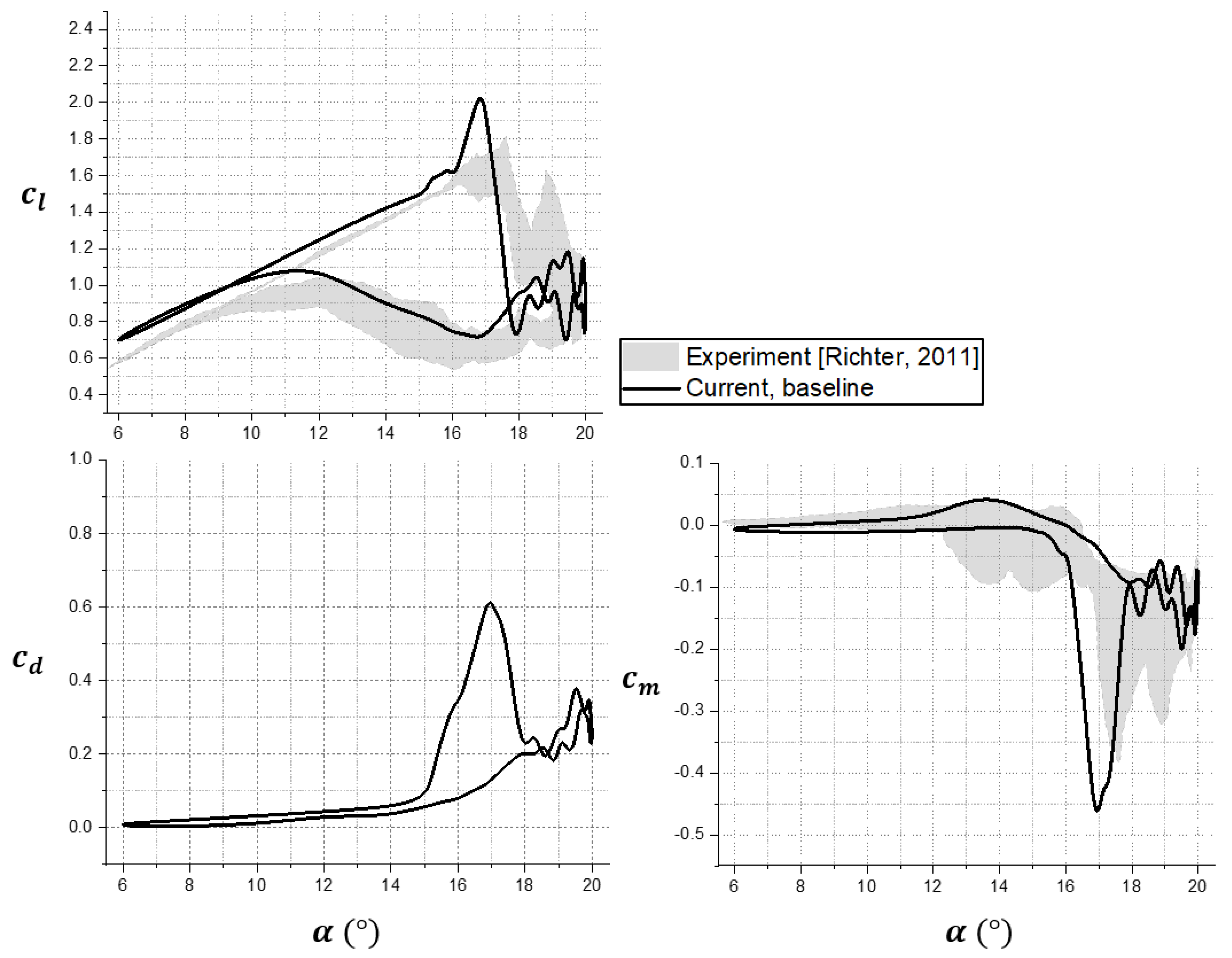
3.1.1. Baseline (No Flow Control)

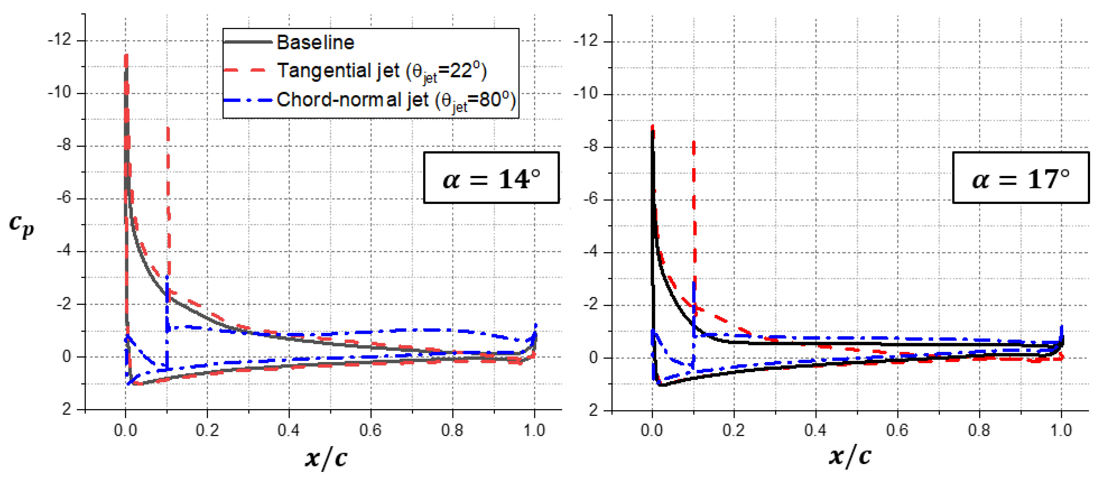
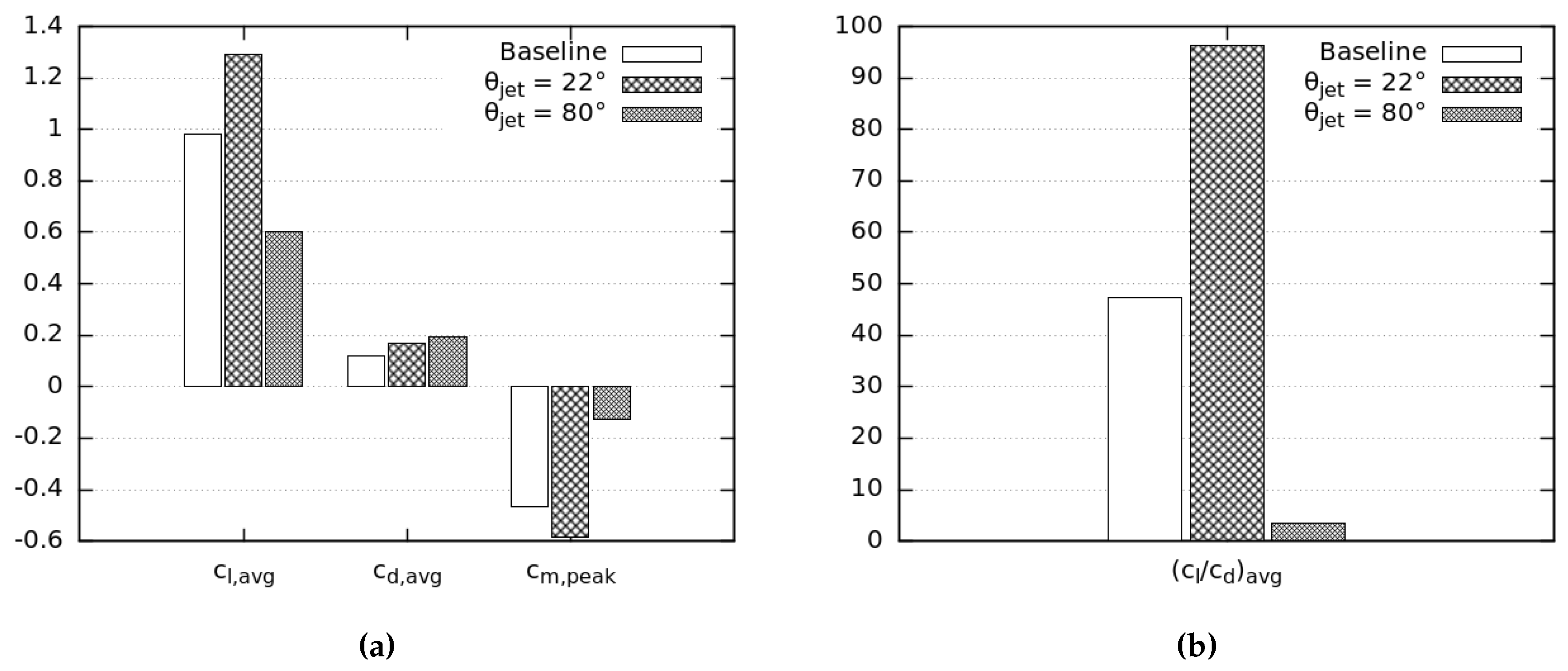
The OA209 airfoil is computed with the compressible Navier-Stokes solver SU2 in rotorcraft-relevant flow conditions: $Ma=0.3,Re=1.15$ M and $0°\le \alpha \le 20°$. The current simulation predicts the static stall angle $\alpha \simeq 14°$, the maximum lift coefficient $c_{l,max}\simeq 1.3$, and the post-stall lift, as shown in Figure 3. It can be conjectured that the noticeable difference to the test in the linear lift region is related to 3D effects in the wind tunnel test, which cannot be modeled in the current 2D simulation (see Figure 3). The current simulation follows the theoretical lift slope $\frac{d{c}_l}{d\alpha }=\frac{2\pi }{\sqrt{1-M{a}^2}}$ in the linear region, whereas the test data slightly deviate from the theoretical line.

Considering 2D environment, it should be note that the agreement to the test data [36] is remarkably improved in the current simulation, compared to other simulations for the same airfoil [19,37] in Figure 3. The agreement on the aerodynamic moment $c_m$ is acceptable. The drag coefficients are also well-predicted with values before the stall angle which was tested.

Pressure profiles between the test and the current computations are compared, as shown in Figure 4. The current pressure profiles at $\alpha =5,14,$ and 19° are agreed well to the available test data. The current simulation slightly overestimate the suction peak, resulting in a slightly higher lift in the linear slop region in Figure 3. Based on 3D simulation of Richter et al. [37], the wind tunnel experiments [36] involve small, but non-negligible 3D efforts primarily due to a tip flow near side walls, which slightly reduces the lift compared to the 2D case.

Current stall phenomena are related to a supersonic pocket near the leading edge at high angles of attack (see Figure 5). The presence of the shock in the accelerated flow is expected because the suction peak at the stall angle $\alpha =14°$ is lower than the critical pressure coefficient $c_p^{*}=-6.9$ in both the experiment and the simulation (see Figure 4). The shock near the leading edge thickens the boundary layer, if it does not immediately cause the flow separation, which is prone to separation under an adverse pressure gradient downstream. It should be emphasized that the current good agreement to test data do not imply that the current SA RANS approach should be used for prediction of general turbulent flow separation. As Slotnick et al. [41] suggested, the limitation of typical RANS computations over various flow separation cases would require advanced, higher-fidelity approaches for general turbulent flow simulation. For the current flow condition, the accelerated flow near the leading edge may improve the SA RANS prediction on the separation.

The current slot width $w_{jet}/c=0.1\%$ yields a negligible impact on the aerodynamic loading without jet actuation, as shown in Figure 6. The open outlet on the suction side is about $0.1\%c$ and $0.27\%c$ for the chord-normal and the tangential slot, respectively. Since the larger outlet with the tangential slot does not change significantly the baseline aerodynamics, the impact of the chord-normal slot by itself on the baseline would be much smaller.

Since the small outlet of the slot on the suction side does not significantly change the baseline aerodynamics, the two distinct grids (one for the clean airfoil and the other for the slotted airfoil) can be used to check the sensitivity of the current computation to the spatial resolution. The slotted airfoil grid of $1150\times 158$ (external flow part) includes much finer grids in the streamwise direction on the suction side, compared to the clean airfoil grid of $420\times 150$. The boundary layer separates near the refined region downstream of the jet outlet at angles slightly beyond the stall angle. Figure 6 indicates that the current clean airfoil grid is fine enough for this stall simulation. This is expected because very similar grids have shown well-converged results with respect to the spatial resolution in aeronautic stall computations using second-order-accurate flow solvers [21,23,47].

3.1.2. Flow Control

The steady-blowing jet is applied to the OA209 airfoil to control the flow separation. The range of the angle of attack is $0°\le \alpha \le 20°$. Two jet angles are applied to the OA209 airfoil: ${\theta }_{jet}=80°$ for the chord-normal jet and ${\theta }_{jet}=22°$ for the tangential jet. The jet momentum coefficient is $c_{\mu }=0.06$ for both the jet actuations. The jet outlet is located at $x_{jet}/c=0.1$ on the suction side.

The aerodynamic lift, moment and drag coefficients are compared in Figure 7. Tangential jet enhances the lift and reduces the magnitude of the moment. However, the chord-normal jet reduces significantly the aerodynamic lift and the moment, undermining the performance of the baseline airfoil. Furthermore, the chord-normal jet causes a severe drag penalty, whereas the tangential jet is able to increase the lift without a significant increase in the drag.

Flow fields of around the OA209 airfoil at $\alpha =14°$ and 17° are shown in Figure 8 and Figure 9, respectively. The velocity in the chord-wise direction $u_x$ and the spanwise vorticity ${\omega }_z$ are used for the visualization. Please note that $\alpha =14°$ is close to the maximum lift angle in both the simulation and the test (see Figure 3). The overall baseline flow is attached on the airfoil at $\alpha =14°$ with a noticeable shallow separation near the trailing edge. The external flow is significantly deteriorated with the chord-normal jet which penetrates the boundary layer, forming a virtual wall. In contrast, the tangential jet remains successfully in the boundary layer. It can be expected that an additional momentum is provided directly into the boundary layer when the jet is ejected at an angle close to the direction of the flow. The vorticity field indicates that the tangential jet resides in the boundary layer with a minimum impact on the boundary layer thickness.

The baseline stall is clearly visible at $\alpha =17°$ with the negative-velocity region and the large stall vortex on the aft airfoil (see Figure 9). The separated flow is well attached on the airfoil with the tangential jet even at this high angle of attack. The vorticity field with the tangential jet at $\alpha =17°$ is visually similar to the baseline and the tangential-jet case at $\alpha =14°$, yielding the similar lift $C_l\simeq 1.2-1.4$.

The gain in the flow momentum due to the jet can be diagnosed with the shape factor H of the suction-side boundary layer. The shape factor is the ratio between the displacement thickness ${\delta }^{*}$ and the momentum thickness $\theta$ in the boundary layer, i.e., $H={\delta }^{*}/\theta$. A small value of H indicates that the momentum of the boundary layer is high enough to withstand an adverse pressure gradient. As shown in Figure 10, the value of H for the chord-normal jet case is over 300 at $\alpha =14°$. In contrast, H for the tangential jet case is even lower than the baseline without flow control. Thus, the tangential jet can help to avoid the separation by providing additional momentum into the boundary layer directly. At $\alpha =17°$, the OA209 airfoil is completely stalled with the separation point at $x/c=0.2$. The tangential jet delays the separation to the mid-chord point, significantly reducing the value of the shape factor, i.e., adding the momentum into the boundary layer without a significant increase in the thickness. The suction side is prone to separation when the shape factor is about 4 in the current simulation.

Pressure profiles are shown in Figure 11 for the two angles $\alpha =14°$ and 15°. At $\alpha =17°$ which is 3° higher than the baseline stall angle, the tangential jet reduces the suction pressure in the first half of the suction side, increasing the lift by $\Delta C_l\approx 0.2$ (see Figure 7). The augmentation of the lift in the first half is related to the pitch-up moment $\Delta C_m\approx 0.03$ which is observed in Figure 7. The chord-normal jet impairs the suction pressure, losing the aerodynamic lift for an angle $\alpha >4°$.

Additional computations are conducted for the tangential jet actuation using a coarse grid (see Figure 12). The total grid count of the coarse grid is about only a quarter of the grid count of the initial fine grid. Only selective angles near and beyond the baseline stall angle are simulated on a coarse grid. The coarse grid provides similar aerodynamic forces obtained from the fine grid, particularly beyond the stall angle. Near the stall, computational results vary slightly due to the spatial resolution, which is not surprising because the boundary layer separation from a smooth surface is indeed sensitive to numerical methods including the spatial resolution.

3.2. Pitching Airfoil Simulations

3.2.1. Baseline (No Flow Control)

The baseline case of no flow control is simulated for the OA209 airfoil with the pitch motion of $\alpha =13\pm 7°$. Since the peak angle $\alpha =20°$ is 6 degrees higher than the static stall angle ${\alpha }_{stall}=14°$, this pitch motion yields deep dynamic stall as shown in Figure 13. Both the moment and lift stall occur beyond the static stall angle. The OA209 airfoil encounters the moment stall around $\alpha =16°$ due to the convection of DSV toward the trailing edge. The aerodynamic lift continuously increase up to $C_{l,max}\approx 2.0$ in the simulation, and the lift stall occurs around $\alpha =17°$ due to the detachment of DSV from the airfoil. The pitching OA209 airfoil experiences oscillatory loads for the range of $18°\le \alpha \le 20°$. The drag peak coincides with the lift peak in the upstroke due to the presence of DSV on the suction side. Further details for the deep dynamic stall are described in the introduction with Figure 1.

The current RANS simulation is able to capture major features observed in the wind tunnel experiment of Richter et al. [38] (see Figure 13). The shaded area indicates the range of the experimental data points [38]. This clearly shows that the dynamic stall in the experiment is not same every pitch cycle. It can be conjectured that the nature of the flow separation associated with the stall and, as a consequence, massively separated flow is highly sensitive to environment and detailed experimental conditions. Nonetheless, the overall aspect of the deep dynamic stall is acceptably reproduced in the current simulation. The moment stall around $\alpha =16°$ and the lift stall around $\alpha =17°$ are captured in the simulation. The magnitude of the peak moment and the peak lift are slightly over-estimated in the simulation. In the upstroke, the current simulation predicts higher $C_l$, compared to the test, which is presumably related to the deviation of the experimental data from the theoretical lift slope for the static airfoil (see Figure 3). No drag data is reported from the wind tunnel experiment.

Similar to the static baseline, a supersonic pocket is observed in this pitching conditions (see Figure 14). The supersonic region already forms at the mean angle, continuously grows till $\alpha \simeq 15°$. Once the DSV separates from the airfoil, the supersonic pocket disappears.

3.2.2. Flow Control

The steady-blowing jet is applied to the OA209 airfoil under the deep dynamic stall. The two jet angles, ${\theta }_{jet}=80°$ and ${\theta }_{jet}=22°$, are used, same to the static case. As shown in Figure 15, the lift is significantly enhanced both in the upstroke and the downstroke by the tangential jet. Entire lift coefficients are improved, compared to the baseline during the upstroke. Additionally, the lift recovers at higher angles around $\alpha =14°$, compared to the recovery angle $\alpha \approx 10°$ in the baseline. The lift and moment loops in the baseline include one major stall, whereas these loops in the tangential-jet case include two major stalls, showing two distinct peaks in each loop. Although the significant rise in the lift is worthwhile, additional event of the dynamic stall due to the tangential jet is not desirable in the control aspect. The amplitude of the negative moment peak is not reduced with the tangential jet. As the lift stall is delayed with a higher lift peak with the tangential jet, the drag divergence is also delayed in the upstroke, which is expected as a common feature of dynamic stall [4].

The chord-normal jet reduces the lift significantly. The degrade in the lift is similar to the static case. The moment coefficient around $c_m\simeq -0.1$ in the pitch cycle without a distinct peak, which is preferable in rotor blade control. The low oscillatory moment, however, comes with a detrimental lift reduction—the hysteresis lift is even lower than the downstroke lift of the baseline.

The evolution of the vorticity ${\omega }_z$ around the pitching OA209 airfoil is compared, as shown in Figure 16. The zero phase $\varphi =0$ corresponds to the mid-upstroke angle $\alpha =13°$. The onset of DSV due to the leading edge separation is visible at $\alpha =15.4°$ in the upstroke of the baseline. The tangential jet delays the DSV onset which occurs around $\alpha =17°$ when the DSV in the baseline is being detached from the airfoil. The DSV in the case of the tangential jet separates from the airfoil after $\alpha =18°$ in the upstroke. Around the peak angle $\alpha =20°$, the tangential jet is dynamically interacted with stall vortices. For example, at $\alpha =20°$, the tangential jet penetrates deeply the re-circulation region. It is interesting to notice the similar presence of the jet in the massively separated region at both the peak and the downstroke angle $\alpha =17.5°$. The interaction between the tangential jet and the separating flow may induce the formation of the secondary DSV at $\alpha =19.8°$ in the downstroke. The maximum size and the strength of the secondary DSV are anticipated to be similar to those of the initial DSV, based on the secondary moment and lift stalls in the case of the tangential jet (see Figure 15). The tangential jet helps the external flow to reattach on the airfoil around $\alpha =15.4°$ in the downstroke, which is even before the mean pitch angle (also the static stall angle without flow control). The suction-side boundary layer without the flow control is still in the re-attachment process at the mean pitch angle $\alpha =13°$.

The chord-normal jet causes a massive flow separation near the jet location during the overall pitch cycle. Similar to the static stall, the chord-normal jet disrupts the external flow, forming a virtual wall with the strong jet with the high jet angle with respect to the freestream direction. It can be postulated that a high-velocity jet with such a large jet angle distributed uniformly in the span is not preferable for the stall control. It should be, however, noted that a discrete distribution of the high-angle jet in the span can avoid the negative disruption on the external flow. As Gardner et al. [17] investigated, a discrete jet can generate secondary vortices in the span which help the mixing of the low-momentum boundary layer flow with the high-momentum freestream flow, and eventually suppress both the static and dynamics stall. Numerical study of a high-angle jet discretely distributed in the span requires three dimensional computations, not pursued in the current investigation.

The flow control case with the tangential jet is further investigated at several major events in the pitch cycle (see Figure 17). This analysis is similar to the baseline shown in Figure 1 in the introduction. As the airfoil pitches up beyond the static stall angle (from stage 1 to 2 in Figure 17), the lift increases continuously due to the well attached flow on the suction side. At stage 3, the initial DSV grows to almost its maximum size, causing the first moment stall while elevating the lift and the drag. From stage 3 to 4, the initial DSV separates from the airfoil, resulting in the first lift stall. In the downstroke, the secondary DSV forms and grows to its maximum size around stage 5, which leads to the second moment stall and the second lift peak. As the secondary DSV detaches from the airfoil, the second lift stall occurs at stage 6. The tangential jet interacts dynamically with the separating flow even at the relatively low angle of stage 7 in the downstroke. For the sufficiently small angle at stage 8, the suction-side flow reattaches on the airfoil.

Several key parameters associated with the aerodynamic coefficients are computed with and without flow control, as shown in Figure 18. The cycle-averaged lift with no actuation is $c_{l,avg}\simeq$ 0.97. In the case of the tangential jet, $c_{l,avg}\simeq$ 1.29, about 33% increase from the baseline lift. The tangential jet also increases the average drag $c_{d,avg}\simeq 0.17$, about 42% increase from the baseline drag. It should be mentioned that the lift-to-drag ratio during the cycle increases drastically with the tangential jet. This is because (1) the lift is enhanced at low angles of attack when the drag remains small and (2) the drag increase is accompanied with the lift enhancement at high angles in the pitch (see Figure 15). The chord-normal jet depreciates the average lift $c_{l,avg}\simeq$ 0.6. Therefore, the overall aerodynamic performance of the OA209 airfoil is improved with the tangential jet.

A tangentially blowing jet is preferable for most of the pitch cycle, significantly increasing the aerodynamic lift and the lift-to-drag ratio. Despite the favorable aspect of the tangential jet, it minimally affects the magnitude of the stall vortex—the peak moment is not reduced with the tangential jet. Additional jet actuation may enhance the control authority further. The chord-normal jet can be effective in suppressing the moment stall, if the jet is generated briefly when the stall vortex breakdown is susceptible to this high-momentum jet. Furthermore, it can be speculated that active variation of the jet angle could enhance the lift and suppress the peak moment. Active control of the jet angle can directly suppress the growth of the DSV, breaking it into smaller and weaker vortices. Such elaborate control methods may also help to avoid the double dynamic stall events which occur in the current case of the tangential jet actuation.

3.2.3. Estimate of Power Benefit with Jet Actuation

Benefit of the current tangential jet for the dynamic stall is estimated. In this estimation, the power input for the generation of the tangential jet is computed, following Gardner et al. [19]: $W_{jet}=ln\left(\frac{P_t}{P_{\infty }}\right)\frac{R{T}_{\infty }{\dot{m}}_{jet}}{2}$ where $W_{jet}$ is the power required for the jet generation per unit span, $P_t=290$ kPa is the total pressure in a compressor, $P_{\infty }=56$ kPa is the current freestream pressure, $T_{\infty }=304$ K is the current freestream temperature, ${\dot{m}}_{jet}=0.24$ kg/(sm) is the mass flow rate per unit span, and R is the gas constant. A constant temperature jet supplied from a constant pressure compressor is used for this power estimation [19]. It is required to provide a power to counterbalance the aerodynamic drag of the pitching airfoil. The drag power per unit span $W_d$ is computed using the formulation $W_d={\int }_0^{T_p}\frac{1}{2}{\rho }_{\infty }{U}_{\infty }^3{c}_d\left(\alpha \right)csin\left(\alpha \right)dt$ where $T_p$ is the period of the pitch. It is expected to gain the lift power using the tangential jet, compared to the baseline. Similar to the drag power, the lift power is computed using the formulation $W_l={\int }_0^{T_p}\frac{1}{2}{\rho }_{\infty }{U}_{\infty }^3{c}_d\left(\alpha \right)ccos\left(\alpha \right)dt$. Please note that the airfoil is projected to a plane normal to the force direction for each the drag and the lift power. The net power is defined as follows $W_{net}=W_l-(W_{jet}+W_d)$. For the baseline and the tangential jet actuation, the aforementioned powers are listed in

Table 3. Estimate of power for jet generation, power to overcome the drag, power from the lift, and the net power during the pitch period.

Case	Wjet [kW/m]	Wd [kW/m]	Wl [kW/m]	Wnet [kW/m]	ΔWnet [kW/m]
Baseline	0	3.9	105.6	101.7	0
Tangential jet	17.2	6.7	137.6	113.7	12.0

.

The benefit of the tangential jet for the dynamic stall is quantified as the net power increase from the baseline $\Delta W_{net}=$ 12 kW/m. The power for generating the strong jet flow of $c_{\mu }=0.06$ is significant, even higher than the power required for negating the drag in the baseline. The benefit of the tangential jet comes from the significant increase in the lift power which overcomes the additional power for the jet and the drag. It is expected because the cycle-averaged lift increases with the jet actuation (see Figure 18). If the jet actuation occurs only in a few right moments during the cycle, not throughout the whole cycle, then the jet benefit $\Delta W_{net}$ could be maximized. Such pulsed jets are of interest in future studies.

4. Conclusions

The effect of the jet angle on flow separation control is investigated for the rotorcraft OA209 airfoil using steady-blowing jets. Two jet angles are used: ${\theta }_{jet}=22°$ for tangential jet and ${\theta }_{jet}=80°$ for the chord-normal jet. Other jet parameters, including the jet location $x_{jet}/c=0.1$ and the jet momentum $c_{\mu }=0.06$, remain the same between the two steady-blowing jets.

The tangential jet can provide additional momentum into the boundary layer directly, reducing the shape factor of the suction side boundary layer. The aerodynamic lift and moment are enhanced beyond the static stall angle for the static airfoil. In contrast, the chord-normal jet deteriorates the baseline aerodynamic performance, severing the external flow.

The tangential jet helps to increase the aerodynamic performance of the OA209 airfoil for the case of deep dynamic stall. The dynamic stall onset is delayed, and, as a result, a higher aerodynamic lift is obtained with the tangential jet, compared to the baseline. The overall increase in the lift-to-drag ratio from the baseline is almost 100%. As with the static stall, the chord-normal jet is not effective in suppressing the dynamic stall.

Although the tangential jet is promising for the suppression of both the static and dynamic stalls, it struggles in reducing the peak moment of the dynamic stall. It can be interpreted that the delayed formation of the dynamic stall vortex does not yield any major modification of the stall vortex strength. Either active variation of the jet angle or multiple jet actuation with various jet angles would attenuate the severe moment stall associated with deep dynamic stall.

References

1. Gault, D.E. A Correlation of Low-Speed, Airfoil-Section Stalling Characteristics with Reynolds Number and Airfoil Geometry; Technical Report NACA-TN-3963; National Advisory Committee for Aeronautics: Washington, DC, USA, 1957.
2. Carr, L.W.; Chandrasekhara, M. Compressibility effects on dynamic stall. Prog. Aerosp. Sci. 1996, 32, 523–573. [Google Scholar] [CrossRef]
3. Johnson, W. Rotorcraft Aeromechanics; Cambridge University Press: Cambridge, UK, 2013; chapter 8.7 Rotor Blade Airfoils; pp. 294–298. [Google Scholar]
4. Leishman, J.G. Principles of Helicopter Aerodynamics; Cambridge University Press: Cambridge, UK, 2006; chapter 9. Dynamic Stall; pp. 525–566. [Google Scholar]
5. Corke, T.C.; Thomas, F.O. Dynamic stall in pitching airfoils: Aerodynamic damping and compressibility effects. Annu. Rev. Fluid Mech. 2015, 47, 479–505. [Google Scholar] [CrossRef]
6. Truong, K.V. Modeling Aerodynamics, Including Dynamic Stall, for Comprehensive Analysis of Helicopter Rotors. Aerospace 2017, 4, 21. [Google Scholar] [CrossRef]
7. Wang, Q.; Zhao, Q. Numerical Study on Dynamic-Stall Characteristics of Finite Wing and Rotor. Appl. Sci. 2019, 9, 600. [Google Scholar] [CrossRef]
8. Harper, P.W.; Flanigan, R.E. Investigation of the Variation of Maximum Lift for a Pitching Airplane Model and Comparison with Flight Results; Technical Report NACA-TN-1734; National Advisory Committee for Aeronautics: Langley Field, VA, USA, 1948.
9. Gadeberg, B.L. The Effect of Rate of Change of Angle of Attack on the Maximum Lift Coefficient of a Pursuit Airplane; Technical Report NACA-TN-2525; National Advisory Committee for Aeronautics: Moffett Field, CA, USA, 1951.
10. Conner, F.; Twomey, W.; Willey, C. A Flight and Wind Tunnel Investigation of the Effect of Angle-of-Attack Rate on Maximum Lift Coefficient; Technical Report NASA-CR-321; NASA: Washington, DC, USA, 1965.
11. Zhu, C.; Wang, T. Comparative Study of Dynamic Stall under Pitch Oscillation and Oscillating Freestream on Wind Turbine Airfoil and Blade. Appl. Sci. 2018, 8, 1242. [Google Scholar] [CrossRef]
12. Li, S.; Li, Y.; Yang, C.; Zhang, X.; Wang, Q.; Li, D.; Zhong, W.; Wang, T. Design and Testing of a LUT Airfoil for Straight-Bladed Vertical Axis Wind Turbines. Appl. Sci. 2018, 8, 2266. [Google Scholar] [CrossRef]
13. Li, S.; Zhang, L.; Yang, K.; Xu, J.; Li, X. Aerodynamic Performance of Wind Turbine Airfoil DU 91-W2-250 under Dynamic Stall. Appl. Sci. 2018, 8, 1111. [Google Scholar] [CrossRef]
14. Zhong, W.; Tang, H.; Wang, T.; Zhu, C. Accurate RANS Simulation of Wind Turbine Stall by Turbulence Coefficient Calibration. Appl. Sci. 2018, 8, 1444. [Google Scholar] [CrossRef]
15. Lachmann, G.V. Boundary Layer and Flow Control; Pergamon Press: Oxford, UK, 1961. [Google Scholar]
16. Gardner, A.D. Investigations of Dynamic Stall and Dynamic Stall Control on Helicopter Airfoils. Ph.D. Thesis, DLR, Deutsches Zentrum für Luft-und Raumfahrt, Cologne, Germany, 2016. [Google Scholar]
17. Gardner, A.D.; Richter, K.; Mai, H.; Neuhaus, D. Experimental investigation of air jets for the control of compressible dynamic stall. J. Am. Helicopter Soc. 2013, 58, 1–14. [Google Scholar]
18. Gardner, A.D.; Richter, K.; Mai, H.; Neuhaus, D. Experimental investigation of air jets to control shock-induced dynamic stall. J. Am. Helicopter Soc. 2014, 59, 1–11. [Google Scholar] [CrossRef]
19. Gardner, A.D.; Richter, K.; Rosemann, H. Numerical investigation of air jets for dynamic stall control on the OA209 airfoil. CEAS Aeronaut. J. 2011, 1, 69. [Google Scholar] [CrossRef]
20. Weaver, D.; McAlister, K.; Tso, J. Control of VR-7 dynamic stall by strong steady blowing. J. Aircr. 2004, 41, 1404–1413. [Google Scholar] [CrossRef]
21. Matalanis, C.G.; Min, B.; Bowles, P.O.; Jee, S.; Wake, B.E.; Crittenden, T.M.; Woo, G.; Glezer, A. Combustion-powered actuation for dynamic-stall suppression: high-mach simulations and low-mach experiments. AIAA J. 2015, 53, 2151–2163. [Google Scholar] [CrossRef]
22. Matalanis, C.G.; Bowles, P.O.; Min, B.; Jee, S.; Kuczek, A.E.; Wake, B.E.; Lorber, P.F.; Crittenden, T.M.; Glezer, A.; Schaeffler, N.W. High-Speed Experiments on Combustion-Powered Actuation for Dynamic Stall Suppression. AIAA J. 2017, 55, 3001–3015. [Google Scholar] [CrossRef]
23. Jee, S.; Bowles, P.O.; Matalanis, C.G.; Min, B.; Wake, B.E.; Crittenden, T.; Glezer, A. Computations of Combustion-Powered Actuation for Dynamic Stall Suppression. In Proceedings of the 72nd American Helicopter Society (AHS) Annual Forum, West Palm Beach, FL, USA, 17–19 May 2016. [Google Scholar]
24. Post, M.L.; Corke, T.C. Separation control on high angle of attack airfoil using plasma actuators. AIAA J. 2004, 42, 2177–2184. [Google Scholar] [CrossRef]
25. Post, M.L.; Corke, T.C. Separation control using plasma actuators: dynamic stall vortex control on oscillating airfoil. AIAA J. 2006, 44, 3125–3135. [Google Scholar] [CrossRef]
26. Amitay, M.; Smith, D.R.; Kibens, V.; Parekh, D.E.; Glezer, A. Aerodynamic flow control over an unconventional airfoil using synthetic jet actuators. AIAA J. 2001, 39, 361–370. [Google Scholar] [CrossRef]
27. Sahni, O.; Wood, J.; Jansen, K.E.; Amitay, M. Three-dimensional interactions between a finite-span synthetic jet and a crossflow. J. Fluid Mech. 2011, 671, 254–287. [Google Scholar] [CrossRef]
28. Chiatto, M.; Capuano, F.; de Luca, L. Numerical and experimental characterization of a double-orifice synthetic jet actuator. Meccanica 2018, 53, 2883–2896. [Google Scholar] [CrossRef]
29. Rice, T.T.; Taylor, K.; Amitay, M. Wind tunnel quantification of dynamic stall on an S817 airfoil and its control using synthetic jet actuators. Wind Energy 2019, 22, 21–33. [Google Scholar] [CrossRef]
30. Huang, L.; Huang, P.; LeBeau, R.; Hauser, T. Numerical study of blowing and suction control mechanism on NACA0012 airfoil. J. Aircr. 2004, 41, 1005–1013. [Google Scholar] [CrossRef]
31. Duvigneau, R.; Hay, A.; Visonneau, M. Optimal location of a synthetic jet on an airfoil for stall control. J. Fluids Eng. 2007, 129, 825–833. [Google Scholar] [CrossRef]
32. Poisson-Quinton, P.; Lepage, L. Survey of French research on the control of boundary layer and circulation. In Boundary Layer and Fow Control; Lachmann, G.V., Ed.; Pergamon Press: Oxford, UK, 1961; Volume 1, pp. 21–73. [Google Scholar]
33. Attinello, J.S. Design and engineering features of flap blowing installations. In Boundary Layer and Flow Control; Lachmann, G.V., Ed.; Pergamon: Oxford, UK, 1961; Volume 1, pp. 463–515. [Google Scholar]
34. Greenblatt, D.; Wygnanski, I.J. The control of flow separation by periodic excitation. Progr. Aerosp. Sci. 2000, 36, 487–545. [Google Scholar] [CrossRef]
35. Greenblatt, D.; Wygnanski, I.J.; Rumsey, C.L. Aerodynamic Flow Control. In Encyclopedia of Aerospace Engineering; Blockley, R., Shyy, W., Eds.; Wiley: Hoboken, NJ, USA, 2010; Volume 1, Chapter 15; Available online: https://onlinelibrary.wiley.com/doi/pdf/10.1002/9780470686652.eae019 (accessed on 31 May 2019).
36. Mai, H.; Dietz, G.; Geibler, W.; Richter, K.; Bosbach, J.; Richard, H.; Groot, K. Dynamic stall control by leading edge vortex generators. J. Am. Helicopter Soc. 2008, 53, 26–36. [Google Scholar] [CrossRef]
37. Richter, K.; Gardner, A.D.; Park, S. Numerical Investigation of the Influence of the Model Installation on Rotor Blade Airfoil Measurements. In New Results in Numerical and Experimental Fluid Mechanics IX; Springer: Berlin, Germany, 2014; pp. 225–233. [Google Scholar]
38. Richter, K.; Pape, A.L.; Knopp, T.; Costes, M.; Gleize, V.; Gardner, A.D. Improved two-dimensional dynamic stall prediction with structured and hybrid numerical methods. J. Am. Helicopter Soc. 2011, 56, 1–12. [Google Scholar] [CrossRef]
39. Economon, T.D.; Palacios, F.; Copeland, S.R.; Lukaczyk, T.W.; Alonso, J.J. SU2: An open-source suite for multiphysics simulation and design. AIAA J. 2015, 54, 828–846. [Google Scholar] [CrossRef]
40. Spalart, P.R.; Allmaras, S.R. A one-equation turbulence model for aerodynamic flows. In Proceedings of the 30th Aerospace Sciences Meeting and Exhibit, Reno, NV, USA, 6–9 January 1992. [Google Scholar]
41. Slotnick, J.; Khodadoust, A.; Alonso, J.; Darmofal, D.; Gropp, W.; Lurie, E.; Mavriplis, D. CFD Vision 2030 Study: A Path to Revolutionary Computational Aerosciences; Technical Report NASA/CR-2014-21878; National Aeronautics and Space Administration: Washington, DC, USA, 2014.
42. Roe, P.L. Approximate Riemann solvers, parameter vectors, and difference schemes. J. Comput. Phys. 1981, 43, 357–372. [Google Scholar] [CrossRef]
43. Venkatakrishnan, V. Convergence to steady state solutions of the Euler equations on unstructured grids with limiters. J. Comput. Phys. 1995, 118, 120–130. [Google Scholar] [CrossRef]
44. Jameson, A. Time dependent calculations using multigrid, with applications to unsteady flows past airfoils and wings. In Proceedings of the AIAA 10th Computational Fluid Dynamics Conference, Honolulu, HI, USA, 24–26 June 1991; p. 1596. [Google Scholar]
45. Gardner, A.D.; Institute of Aerodynamics and Flow Technology, German Aerospace Center (DLR), Coln, Germany. Personal communication, 2018.
46. Pape, A.L.; Costes, M.; Joubert, G.; David, F.; Deluc, J.M. Dynamic stall control using deployable leading-edge vortex generators. AIAA J. 2012, 50, 2135–2145. [Google Scholar] [CrossRef]
47. Kim, T.; Kim, S.; Lim, J.; Kim, J.; Jee, S. Computational Study of Mach Number Effects on Dynamic Stall. In Proceedings of the ASME-JSME-KSME Joint Fluids Engineering Conference, San Francisco, CA, USA, 28 July–1 August 2019; p. 5536. [Google Scholar]
Figure 1. Static and dynamic stalls of OA209 airfoil at M a = 0.3 , R e = 1.15 × 10 6 and k = 0.05 .
Applsci 09 02960 g001
Figure 2. Grids around the OA209 airfoil, near the leading edge, and near the jet slots. Every 4th point is shown.
Applsci 09 02960 g002
Figure 3. Comparison of the current simulation to the experiment [36] and the SA RANS simulations [19,37] of the clean OA209. M a = 0.3 , R e = 1.15 M.
Applsci 09 02960 g003
Figure 4. Comparison between experimental data [36] and the current simulation of the OA209. M a = 0.3 , R e = 1.15 M.
Applsci 09 02960 g004
Figure 5. A supersonic pocket near the leading edge at three selected angles.
Applsci 09 02960 g005
Figure 6. Comparison between the clean and the tangentially slotted airfoils.
Applsci 09 02960 g006
Figure 7. Static OA209 airfoil with and without steady-blowing jets. M a = 0.3 , R e = 1.15 M, c μ = 0.06 .
Applsci 09 02960 g007
Figure 8. Time-averaged flow field around the OA209 airfoil with and without steady-blowing jets. M a = 0.3 , R e = 1.15 M, c μ = 0.06 and α = 14 ° .
Applsci 09 02960 g008
Figure 9. Time-averaged flow field around the OA209 airfoil with and without steady-blowing jets. M a = 0.3 , R e = 1.15 M, c μ = 0.06 and α = 17 ° .
Applsci 09 02960 g009
Figure 10. Shape factor of the suction-side boundary layer on the OA209 airfoil with and without steady-blowing jets. M a = 0.3 , R e = 1.15 M, c μ = 0.06 at α = 14 ° and 17°.
Applsci 09 02960 g010
Figure 11. Comparison between static OA209 with and without steady-blowing jets. M a = 0.3 , R e = 1.15 M, c μ = 0.06 at α = 14 ° (left) and 17° (right).
Applsci 09 02960 g011
Figure 12. Comparison of two grids for the tangential jet actuation.
Applsci 09 02960 g012
Figure 13. Pitching OA209 airfoil in the test [38] and current simulations. M a = 0.3 , R e = 1.15 M, k = 0.05 and α = 13 ° ± 7 ° .
Applsci 09 02960 g013
Figure 14. A supersonic pocket near the leading edge in the upstroke.
Applsci 09 02960 g014
Figure 15. Pitching OA209 airfoil with and without steady-blowing jets. M a = 0.3 , R e = 1.15 M, c μ = 0.06 , k = 0.05 and α = 13 ° ± 7 ° .
Applsci 09 02960 g015
Figure 16. Vorticity ω z field for the pitching OA209 airfoil with and without steady-blowing jets. M a = 0.3 , R e = 1.15 M, c μ = 0.06 , k = 0.05 and α = 13 ° ± 7 ° .
Applsci 09 02960 g016
Figure 17. The OA209 airfoil with the tangential jet in the static and pitching conditions. M a = 0.3 , R e = 1.15 M, c μ = 0.06 , k = 0.05 and α = 13 ° ± 7 ° .
Applsci 09 02960 g017
Figure 18. Lift (cycle-averaged), drag (cycle-averaged), the peak moment and the lift-to-drag ratio (cycle-averaged) of the pitching OA209 airfoil with and without steady-blowing jets. M a = 0.3 , R e = 1.15 M, c μ = 0.06 , k = 0.05 and α = 13 ° ± 7 ° .
Applsci 09 02960 g018