Abstract
Diffuse correlation spectroscopy (DCS) has widely been used as a non-invasive optical technique to measure tissue perfusion in vivo. DCS measurements are quantified to yield information about moving scatterers using photon diffusion theory and are therefore obtained at long source-detector separations (SDS). However, short SDS DCS could be used for measuring perfusion in small animal models or endoscopically in clinical studies. Here, we investigate the errors in analytically retrieved flow coefficients from simulated and experimental data acquired at short SDS. Monte Carlo (MC) simulations of photon correlation transport was programmed to simulate DCS measurements and used to (a) examine the accuracy and validity of theoretical analyses, and (b) model experimental measurements made on phantoms at short SDS. Experiments consisted of measurements from a series of optical phantoms containing an embedded flow channel. Both the fluid flow rate and depth of the flow channel from the liquid surface were varied. Inputs to MC simulations required to model experiments were obtained from corrected theoretical analyses. Results show that the widely used theoretical DCS model is robust for quantifying relative changes in flow. We also show that retrieved flow coefficients at short SDS can be scaled to retrieve absolute values via MC simulations.
1. Introduction
Diffuse correlation spectroscopy (DCS) is a well-established optical technique capable of sensing blood flow in biological tissue using multiply scattered light and has widely been applied to quantify tissue perfusion in vivo [1,2,3,4,5,6,7,8,9,10,11,12,13]. The light source used in DCS is a long coherence length laser, which is delivered to a medium of interest through a large-core optical fiber while the back-scattered (reflected) intensity is collected using a small-core (single mode) fiber, placed at a fixed distance (the source-detector separation SDS) from the center of the source fiber. The detected signal is transmitted to a photon counter that in turn is electronically coupled to a hardware correlator board [14,15]. Experimental DCS measurements yield the normalized intensity autocorrelation function, measured for a given fiber geometry, which in turn is quantified by fitting via an analytical expression to extract flow-dependent coefficients that characterize the dynamically scattered photon transport [15,16,17].
Theoretically, solutions to the unnormalized field correlation are found by considering it to be governed by the modified photon diffusion equation
As discussed previously [15,16,17], in Equation (1) is the photon diffusion coefficient of the medium (determined from its absorption and reduced scattering coefficients , as ). is a correlation-time () dependent term and represents the ensemble-averaged, mean-squared displacement of moving scatterers in time . is the wave-vector associated with the laser source and describes the spatial geometry of the source to be modeled [15]. Two models are commonly used for : the Brownian flow model (where ) with Brownian flow coefficient ; the random flow model (where ) where is the average volumetric flow-speed of the scattering particles [5,15,16,18,19,20].
In a semi-infinite turbid medium, for a collimated pencil-beam input, closed form analytical solutions to in cylindrical geometry is given by
Here, is dependent on the medium’s absorption, scattering and correlation-transport properties as . and are given as and , where is the SDS (i.e., the distance from the detection point on the surface of the semi-infinite medium and the collimated input source). and are dependent on the medium’s optical properties (via the boundary conditions specified) as and and A is obtained from the relative refractive index between the medium and detector, as discussed previously [17,19,21]. To match theoretical predictions to experimental measurements the unnormalized field correlation is transformed into the normalized intensity correlation via the Siegert relation, which gives that , where , and is a scalar constant that depends on detection geometry [15,16].
Equation (2) is derived from the formalism of photon diffusion theory and as such would be expected to carry constraints on its validity (dictating geometry of measurements and the choice of laser wavelengths) [22,23,24,25,26]. To satisfy these constraints, experimental measurements of DCS typically use long SDS (>1 cm) and near-infrared laser sources. However, there could be clinical opportunities for using endoscopically compatible DCS probes to assess tissue perfusion in vivo, which will need to use short SDS for signal acquisition. Further, recent reports have employed DCS measurements at short SDS (<1 cm) for quantifying tissue perfusion in small animal models [27,28,29,30,31]. Surprisingly, these studies all reported that the classical diffusion-theory based theoretical expression in Equation (2) still provided good parametrization of relative changes in tissue perfusion even at short SDS used. Here, we further investigate the utility of Equation (2) to parametrize absolute and relative changes in flow in turbid media measured experimentally data in controlled flow-phantoms at short SDS. Additionally, we also investigate the use of Equation (2) to parametrize numerically simulated data at short SDS.
Monte Carlo (MC) based modeling of photon migration provide direct, numerical solutions to the radiative transport equation and have been extensively used in the field of tissue spectroscopy [32]. They are well developed and have been used to quantify experimental measurements of diffuse reflectance obtained in phantoms, animal models and human studies [33,34,35,36,37]. MC simulations can be programmed to incorporate heterogeneous tissue architectures and can be used to accurately model diffuse reflectance and correlation even at short SDS [32,38]. Thus, MC based photon transport methods have been used to compute normalized field correlation in semi-infinite media, simulate intensity correlation decays in complex layered scattering media and to validate improved theoretical models [31,38,39,40,41,42].
Here, we first examine the impact of using Equation (2) to quantitatively retrieve from that were simulated using MC models of semi-infinite media spanning a range of absorption, scattering and Brownian flow diffusion coefficient at varying SDS. Next, we acquired DCS measurements at a fixed short SDS of 0.15 cm, experimentally, in a set of flow-phantoms that included an embedded flow-channel (containing the same liquid as the phantom). The phantoms were designed to investigate how two physical parameters—the depth of the flow-channel from the optical probe and the flow type and rate of fluid in the channel—influenced DCS measurements obtained on the surface.
In Section 2, we describe the experimental methods used including the instrumentation, the design of liquid phantoms and the construction of the flow-channel. We then outline the MC modeling approach to simulate photon correlation transport and the tissue models simulated for analysis, discuss the use of Equation (2) to parametrize simulated and experimental data and provide a description of the goodness-of-fit metrics used. Section 3 presents the results of the analysis of the MC simulations of semi-infinite models, followed by results from theoretical analysis of the experimental phantom, and then show the comparison between MC models developed to simulate experimental measurements on flow phantoms.
2. Materials and Methods
2.1. Experiments
2.1.1. Instrumentation
Experimental DCS measurements were obtained using a home-built system that employed a stabilized diode laser centered at 785 nm and coherence length of nearly 3 m (I0785SH0100B-TH-L; Innovative Photonic Solutions, NJ, USA) as the source. The laser was coupled into one end of an SMA terminated fiber (diameter 200 μm, NA 0.22) of a fiber optical probe. The sampling end of the probe consisted of a detector fiber (diameter 8.2 μm) and was custom-fabricated (Gulf Photonics, Oldsmar, FL, USA) with SDS of 0.15 cm. The distal end of the detector fiber was optically coupled to a single photon counting module (ID100; ID Quantique, Geneva, Switzerland), which in turn was electronically connected to a digital correlation board (LS Instruments, Fribourg, Switzerland). The correlator was controlled by a computer and recorded DCS scans as normalized intensity autocorrelation functions, .
2.1.2. Liquid Phantoms
Liquid phantom media with required optical properties were prepared by mixing pre-determined volumes of an absorbing solution (with negligible scattering) and scattering solution (with negligible absorption), and diluting the resulting solution with deionized (DI) water, using protocols described previously [33,43]. A suspension of 1.0 μm diameter polystyrene microspheres (Polybead microspheres, 07310, Polysciences Inc., Warrington, PA, USA) was used as the scatterer and its scattering coefficient was calculated from Mie theory [44]. The absorber solution was prepared by dissolving bovine hemoglobin (H3760; MilliporeSigma, MO, USA) in DI water, whose absorption coefficient was experimentally measured using a transmission spectrophotometer (Cary 100 UV-Vis, Agilent Technologies, Wilmington, DE, USA). The volume-fractions of absorber and scatter mixed together determined the absorption and scattering coefficient of the final solution [33]. The liquid media used for phantoms were prepared with absorption coefficient of = 0.075 cm−1 and reduced scattering coefficient = 12 cm−1. These values for absorption and scattering at 785 nm (the laser wavelength) are within ranges previously reported for different tissue types including bone, abdomen and white matter of the brain [45,46,47].
2.1.3. Flow-Chamber Description
Figure 1a shows a photograph of the phantom used and its schematic illustration in Figure 1b. A plastic chamber with dimensions of 5.5 cm × 5.5 cm × 1.0 cm was filled with the liquid phantom described above (having = 0.075 cm−1; = 12 cm−1 at 785 nm) and the chamber was placed atop a homogenous solid phantom block with similar optical properties as the liquid phantom at 785 nm. The chamber housed a clear plastic tube (inner diameter = 1.6mm, outer diameter = 3.2 mm; 8000–0004; Thermo Fisher Scientific Inc., Miami, OK, USA) that was attached to two opposite sides of the chamber using moldable glue (Sugru; FormFormForm Ltd., London, UK) and ran along the bottom surface of the plastic chamber, parallel to one edge. One end of the plastic tube was connected to a syringe pump (75900–00; Cole Parmer, Vernon Hills, IL, USA) that was controlled via software to produce a given volume flow rate , while the other end of this tube drained into a sink. Assuming laminar flow, the pump flow rate was converted to an average fluid flow speed in the channel as , where is the cross-sectional area of the channel and the flow speed. Since the same liquid phantom added to the chamber was also loaded into the syringe pump, both the actively pumped and surrounding liquid media had identical optical transport coefficients. was set via software to one of four values: (pump turned off; 0 mL/h), (1.44 mL/h), (3.60 mL/h) or (5.76 mL/h). Given a circular tube of radius 0.08 cm, the average channel flow speeds were calculated to be 0.02 cm/s, 0.05 cm/s and 0.08 cm/s at , , and , respectively. These flow rates gave speeds in ranges reported for moving red blood cells in capillaries [48].
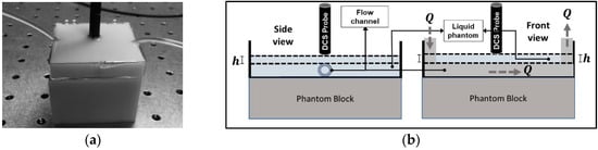
Figure 1.
Photograph of the phantom flow chamber (a) and schematic of the flow chamber’s construction and measurement system (b). The gray arrows in (b) show the direction of the fluid flow. The flow rate F was controlled using a motorized syringe pump (see text). h is the distance from of the liquid surface to the top of the flow channel, which was controlled by addition of specific volumes of the liquid phantom to the chamber. The chamber (edges shown as thick black lines in (b) was placed atop a homogeneous tissue phantom block with optical properties matched to the liquid phantom at the laser wavelength. The DCS probe was positioned directly above the flow channel and at center of the flow chamber.
2.1.4. Phantom Preparation and Measurement Protocol
Two primary parameters were varied in the flow phantoms as shown in Figure 1b—the volume flow rate through the flow channel and the depth of the flow channel from the fluid surface. The flow rate was cycled through for four rates (–), for four cycles. The depth of the flow-channel from the liquid surface was held fixed (from to ) for each flow speed cycle.
The plastic flow chamber had equal length and breadth ( 5.5 cm), thus addition of a given volume of liquid to the chamber would raise the height of the fluid surface by . For the first phantom to be measured, the chamber was filled with prepared liquid media such that liquid surface was visually assessed to have just submerged the flow channel. The depth of the flow channel for this first phantom was assumed to be . DCS measurements were acquired in this phantom by cycling through the four different flow rates (–), giving four measurements (labeled –).
Next, 1.0 mL of phantom was added to the container, which was estimated to increase the depth of the channel from the surface by approximately = 0.03 cm, as done previously [49]. The depth of the flow channel from fluid surface was . DCS measurements were acquired for a full cycle of pump volume flow rates (–) and gave phantoms –. The process was repeated twice—each time, 1 mL of liquid was added to the chamber (increasing depth of channel by and ). Thus, DCS measurements were obtained for 16 phantoms, corresponding to each depth and flow-rate used and were sequentially measured in sets of 4, starting from - and ending in -. It is worth noting that this experimental protocol implied that in all but the first set of four measurements, the pump had been active for at least one cycle of operation before additional media was added to the chamber (i.e., was measured chronologically after ).
2.1.5. Data Acquisition
For each phantom, prepared phantom liquid media (with viscosity nearly that of water) was added to the container, stirred gently and allowed to come to rest (3–5 min). DCS measurements were obtained by moving the optical fiber probe vertically toward the liquid surface. The probe was situated at the center of the phantom container and oriented such that the line connecting the center of the source and detector fiber was perpendicular to the flow channel and was positioned using custom probe holder (mounted on a linear optical stage that allowed the probe head to be moved away or toward the liquid surface). Once the liquid phantom was prepared, the probe was moved till it just broke the surface tension of the liquid medium. Five scans were recorded for each phantom with changing flow condition. Each DCS scan was acquired for 1s and had count rates ranging between 80–100 kHz. The probe was then removed, new media added, and the process repeated for depths –.
2.2. Monte Carlo Simulations of Correlation Transport
Light propagation in tissue-like media can be numerically simulated by construction of stochastic trajectories of individual photon packets, where the variables governing the evolution of these trajectories are determined by an input tissue model’s optical properties and sampled using MC techniques [32,50]. In these simulations, several (106–108) individual photon packets are launched and aggregate quantities of interest (such as the photon flux, fluence, absorbance and fluorescence) are tracked spatio-temporally, for a given tissue model. For the studies here, we modified a time-resolved MC photon transport model (previously described in detail [49,51]) to include simulate of photon field correlations in reflection geometry. We note that MC modelling of photon transport in scattering media are well discussed elsewhere [50,51], and we therefore confine description of aspects pertinent only to tracking of field correlations in the MC model.
Correlation transport was integrated into the MC model by adding a new variable (programmed into the simulation) to track the field correlation carried by each photon packet, as it was transported from the source to the detector, following the methodology described before [15,39,40]. To track the decay of the normalized photon-field correlation , it was assumed that moving particles were uniformly distributed in each tissue layer modeled, moved uncorrelated to each other and that all photon scattering events were from dynamically moving particles. Under those conditions, was expressed as
In Equation (3), represents the mean-squared displacement term of particles contributing to dynamic scattering in time , while is the magnitude of momentum transfer due to a scattering event. Each scattering event undergone by a photon packet tracked in the MC simulation provides specific associated with it. Thus, in the geometry of the MC model, if and represented directions associated the incoming and scattered photon packets, then , where is the single-scattering angle (i.e., the angle between and ) sampled by the MC model, for the photon packet being tracked [15,40]. Since , and (the wavelength of the laser) is known, Equation (3) was used to update this variable, through the flight of the photon packet simulated using
In Equation (4) the superscripts and refer to the field correlation variable (for a given photon packet within the MC simulation) before the and scattering event, respectively with being computed at the scattering event. was the mean-squared displacement of the scattering particles in layer (where the scattering event occurred) and was set either to for Brownian flow, or to for random flow [15]. Thus, inputs to the MC simulations (for each layer) required flow coefficients (or ) together with the layer optical properties. in Equation (4) was computed (depending on inputs either as Brownian or as Random flow) dynamically, through the path of each photon packet tracked.
Each photon packet launched had initial value of . If a photon packet exiting the medium was detected by the simulation, the photon packet’s field correlation variable was multiplied with the exiting photon weight (to account for all path-length dependent absorption losses) and accumulated into a global field correlation variable, , where indexed the spatial detector location for the exiting photon. At the end of the simulation, was normalized such that (i.e., was divided by the number of photons detected, for each detection-bin). The MC model used here yielded surface reflectance for photons exiting into annular, concentric rings on the surface of the medium ( identifies the distance of the collection annulus from relative to a source at the origin).
2.3. Tissue Models Simulated
2.3.1. Semi-Infinite Models
The first set of simulations consisted of 210 runs modeling different semi-infinite media with each run producing for 20 SDS (uniformly spaced between 0.1–2 cm). The optical properties of the media simulated obtained by permuting through five scattering coefficients (: 3 − 15 cm−1), seven absorption coefficients (: 0.05 − 0.5 cm−1) and six Brownian flow coefficients (: 5 × 10⁻⁹–3 × 10⁻⁸ cm2/s) following the ranges as reported recently [31]. These MC simulations were compared against theoretical calculations to assess both the predictions of theory (forward model), as well as parametrization of the simulations (inverse model), as described in Section 2.4.
2.3.2. Three-Layer Models
The second set of MC simulations modeled experimental measurements. Each measurement from a phantom (for given depth and flow speed) was modeled as a 3-layered slab (following the schematic in Figure 1b). Layer 1 was liquid covering the flow chamber, whose layer thickness represented depth of channel from surface. Layer 2 was the flow channel having fixed thickness of 0.15 cm (to match the inner diameter of the tubing used) and Layer 3 representing the solid phantom block (thickness of 5 cm).
We note that this modeling architecture does not account for the plastic tube-wall (present experimentally). Modeling the tube wall as an additional layer with (with low values of absorption, scattering and Brownian correlation-decay coefficient relative to the liquid layer) did not change simulated outputs relative to an equivalent 3-layer model and thus we chose to represent flow phantoms as a 3-layer model. Since Layer 1 and Layer 2 contained the same liquid medium, and since the optical coefficients for Layer 3 (solid block) was similar to that of the liquid phantom, we modeled all layers as having identical transport coefficients and refractive indices, matching those of the liquid phantom used.
Table 1 shows the required inputs (with values for experimentally known parameters) needed to simulate photon correlation from the three-layer phantom models. In Layers 1 and 3 the correlation flow coefficients were modeled as diffusive with a given Brownian diffusion coefficient; for Layer 2 it was modeled as diffusive only when the pump was inactive (phantom ). The flow in Layer 2 was modeled as random flow, when the fluid was actively pumped. The Brownian flow-coefficient inputs for layers 1 and 3 were kept fixed for all flow speeds (for fixed depth). Input values of all Brownian flow coefficients needed were obtained using theoretically analyses (described in Section 3.3.1).

Table 1.
Optical coefficients used for simulations of three-layered tissue models.
Increasing depth of the flow channel were modeled via MC simulations by increasing the thickness of Layer 1 (from ) in increments of 0.03 cm, to match experimentally expected values. The thickness of layer 1 at depth needed to be empirically determined (described in Section 3.3.2). Changes in channel flow rates were modeled by varying flow coefficients used for Layer 2 such that the relative change in flow / and / in the MC models matched experiments. The flow speed in Layer 2 at flow rate (1.44 mL/h) was needed and was also empirically determined (described in in Section 3.3.2). MC predictions of simulated for experimental phantoms were obtained for the experimental SDS of 0.15 cm.
2.4. Theoretical Analyses
Both the simulated and measured data were presented as normalized intensity field correlation for theoretical analyses. Since measurements provide normalized intensity correlations, the theoretical unnormalized field correlation from Equation (2) was transformed into the intensity correlation via the Siegert relation ( as mentioned before [15,16] and thus experimental data were fitted using Equation (2) via a non-linear least-squares optimizing algorithm (lsqcurvefit in MATLAB) to retrieve coefficients describing and .
Two functional forms used previously to describe were used—the Brownian flow model or the random-flow model [16,17]. When scatterers are assumed as moving diffusively in the medium . Scatterers moving under actively pumped flow are modeled as random flow with . These two flow models can also be combined together as a shear-flow model where the mean squared displacement contains both terms, [52]. Experimental data were analyzed using three flow models: for Brownian flow model was obtained, for the random flow the speed of the particles was obtained, and for the shear-flow model both coefficients and were obtained. All other variables needed to evaluate Equation (2)—i.e., the optical properties of the medium, SDS, refractive index of medium and detector—were set matched to experimentally used values.
Equation (2) was used in two ways to analyze MC simulated data. The first (as forward model) was to employ it to calculate from inputs of a given simulation, to match it directly against to MC simulations (at any needed SDS). The second way was as the inverse model as used for the analysis of experiments. However, to keep this procedure identical to processing of experimental data, simulated data were first translated into (using a fixed value of = 0.48) before least-squares fitting. As in the experimental analysis, the fit coefficients describing and were obtained. All other variables needed to evaluate Equation (2)—i.e., the optical properties of the medium, SDS, refractive index of medium and detector—were matched to simulated inputs.
2.5. Goodness-of-Fits: Fit Residuals
The results of fitting the measured, simulated and calculated correlation functions across the different experimental phantoms and MC models were quantified by using a non-negative scalar value , as a measure of the goodness-of-fit. This was calculated as , where was the intensity correlation (measured or simulated) and was the fitted intensity correlation (using Equation (2) or simulated). A perfect fit would have , and thus the lower the the better the goodness-of-fit. The index corresponds to discrete correlation-time bins (as output by the hardware correlator using a multi-tau data accumulation scheme). For analysis here, there were a total of logarithmically spaced bins (i.e., the correlation times were evenly spaced on a log scale), matching experimental data with μs and s.
3. Results
3.1. Simulations in Semi-Infinite Phantoms
3.1.1. Forward Theoretical Calculations vs. Simulations
Figure 2 presents direct comparisons of MC simulated (symbols) and forward calculations using Equation (2) (lines). Each plot shows data from five different tissue models (squares: = 3/cm; triangles: = 6/cm; circles: = 9/cm; asterisks: = 12/cm; diamonds: = 15/cm). Figure 2a,b show data for media with absorption = 0.05/cm, at SDS of 0.15 and 1.5 cm respectively. All simulated and theoretical models shown in Figure 2 had fixed Brownian flow coefficient of = 2 × 10⁻⁸ cm2/s. Data in Figure 2c,d) are for media with higher absorption = 0.42/cm, at same SDS as Figure 2a,b respectively. The fit-residuals are shown within legends for each simulated model in Figure 2a and d and are in accordance with known limitations of diffusion theory—i.e., data simulated for long SDS were fit better Figure 2c,d, relative to data from shorter SDS Figure 2a,c and simulated media with lower albedo (where the albedo ) were fit worse relative, to media with higher albedo.
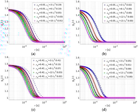
Figure 2.
MC simulations (symbols) and forward theoretical calculations using Equation (2) (lines) for media with low and high absorption (top and bottom rows) at SDS of 0.15 and 1.5 cm (left and right columns). Each figure shows data for 5 media with varying scattering distributed between = 3/cm (squares) to = 15/cm (diamonds).
3.1.2. Fitting Simulations Using Theory
Direct calculations of from diffusion theory deviated at short SDS relative to MC predictions, but Equation (2) could be instead used to freely fit simulated data for the Brownian diffusion flow coefficient as described in Section 2.4. Symbols in Figure 3a–d show the same simulated data as in Figure 2a–d, respectively, while lines show fitted diffusion theory calculations. It is clear that the theoretical data fit simulations near perfectly, even at short SDS of 0.15 cm Figure 3a,c and for low albedo media. Although the numerical fits in Figure 3 matched numerical simulations much better than direct forward calculations Figure 2, these numerical fits are obtained at the cost of errors in retrieved flow coefficients.
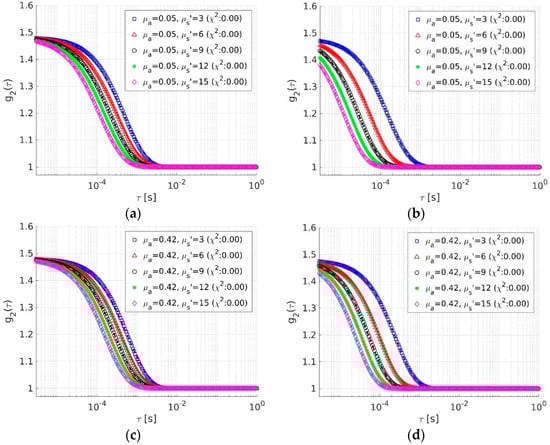
Figure 3.
MC simulations (symbols) with fitted curves using Equation (2) (lines) via optimizing for the Brownian flow coefficient (inverse model) to minimize residuals. Simulated data shown in (a,d) are identical (in the same order) as Figure 2a,d. Data in (a,c) are for SDS of 0.15 cm (at low and high absorption coefficients respectively), while data in (b,d) are for SDS of 1.5 cm.
3.1.3. Errors from Theoretical Fits
In Figure 4, retrieved values of the absolute Brownian flow coefficients (from each fit) are shown as contour maps from 35 simulations (spanning 7 absorption and 5 scattering coefficients) with fixed Brownian flow coefficient = 2 × 10⁻⁸ cm2/s, for three different SDS (Figure 4a: SDS = 0.15 cm; Figure 4b: SDS = 0.45 cm; Figure 4c: SDS = 0.75 cm). With decreasing SDS, the retrieved values of increased from its expected (known) value of = 2 × 10⁻⁸ cm2/s. Figure 4d–f show the same data as Figure 4a–c, but as percent-errors relative to the true input value (of = 2 × 10⁻⁸ cm2/s). As seen before, errors associated with retrieved flow coefficients were highest for small SDS and low albedos. These data also indicate that extracted depended on the optical properties of the media, and the SDS used.
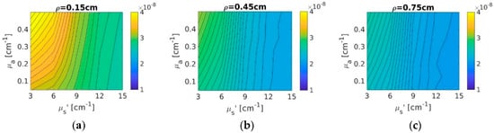
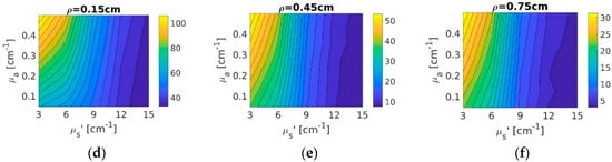
Figure 4.
Retrieved flow coefficients obtained via using Equation (2) to fit simulations (top-row) and corresponding percent-errors (bottom-row) for 35 different MC simulations spanning seven and five values and fixed = 2 × 10⁻⁸ cm2/s. Data are shown as contour maps for 3 different SDS (left column: SDS = 0.15 cm; middle column: SDS = 0.45 cm; right column: SDS = 0.75 cm). Note that the color-bar scale is fixed for the top row but changes across SDS for the bottom row.
Figure 5 shows the averaged percent-error for extracted with varying SDS, for the six coefficients simulated (squares: 5 × 10⁻⁹ cm2/s; up-triangles: 1 × 10⁻⁸ cm2/s; circles: 1.5 × 10⁻⁸ cm2/s; asterisk: 2 × 10⁻⁸ cm2/s; diamonds: 2.5 × 10⁻⁸ cm2/s; down-triangles: 3 × 10⁻⁸ cm2/s). For each line (i.e., at fixed ), the percent errors at each SDS shown in Figure 5 was the mean across all 35 simulated models (spanning seven and five values with given ), while error-bars are standard-deviations. Abscissa of each line (for each ) are shown staggered in Figure 5 to show six distinct markers, since the computed errors (and distributions) were nearly identical across all values. In other words, the percent-error in retrieved was independent of the flow coefficient used and only depended on the optical properties of the medium and the SDS used. These data are in agreement with findings published in a recent report that investigated short separation DCS with MC simulations [31].
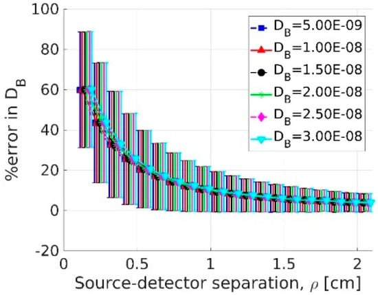
Figure 5.
Percent-errors in retrieved Brownian flow coefficient with varying SDS from analysis of simulations. Lines show data for 6 simulated coefficients (identified in the legend). Symbols represent mean percent errors calculated across all available simulations for given SDS and , while error bars shows standard deviations. Data for each point (in each line) was computed across 35 simulations run (see text) with varying absorption and scattering. The lines were identical to each other and are shown staggered only for visual clarity.
3.1.4. Relative Changes in Flow Coefficients: Simulations vs. Theory
Even though there were errors in absolute values of retrieved coefficients when simulations at high albedo and/or short SDS were fit with Equation (2), relative changes in derived flow coefficients could be compared in media with given (fixed) optical scattering and absorption but changing . Figure 6 shows the mean relative change in extracted coefficient, at three different SDS—where the relative change in at each SDS, was calculated as the ratio of the retrieved coefficient for a given simulation (i.e., for given medium optical coefficients), by the retrieved from a matched simulation but with = 5 × 10⁻⁹ cm2/s. The mean value of the relative changes in thus calculated across each of the 35 simulations (spanning all 7 and 5 coefficients) are shown by three bars, each for different SDS in Figure 6. The red asterisks indicate error bars computed as the standard deviation across each of these 35 simulations and were nearly zero, indicating that predicted relative changes in values from theoretical analyses, were near exactly as modeled by the simulations, across all SDS.

Figure 6.
Relative change in extracted flow coefficients (relative to values obtained from media simulated with = 5 × 10⁻⁹ cm2/s) at three different SDS. The true relative change in (x-axis) was obtained from input values to simulations, while the derived values (y-axis) were obtained from fitted coefficients (see text).
3.1.5. Scaling Factors: Linearly Correcting Retrieved Coefficients
Given relative changes in could be computed across optically identical media but with different flow coefficients, we derived correction factors (for each medium with given optical coefficients and required SDS). These correction factors were calculated as the ratio of the simulated (input) Brownian flow coefficients simulated, to the flow coefficient retrieved via fitting the simulation using Equation (2). Thus, retrieved coefficients, for any medium, could be appropriately scaled and corrected to estimate an absolute flow coefficient. Figure 7 shows the correction factor maps obtained (across the 35 simulated media) at two different input coefficients (Figure 7a,c: = 1 × 10⁻⁸ cm2/s; Figure 7b,d: = 3 × 10⁻⁸ cm2/s) for two different SDS (Figure 7a,b: 0.25 cm; Figure 7c,d: 1.05 cm). The similarity of these derived correction factors in Figure 7a–d indicate that they were nearly identical for either flow coefficient. Since a correction factor of unity would indicate that retrieved flow coefficient was the same as that modeled, the correction factors in Figure 7a,b (short SDS) are correspondingly lower, than those for Figure 7c,d (longer SDS).
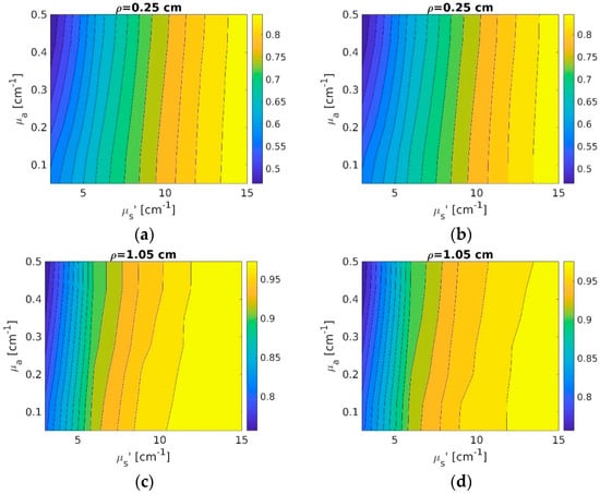
Figure 7.
Scaling (correction) factors determined using simulations at two SDS (top: 0.25 cm; bottom: 1.05 cm) shown for two different media with two different flow coefficients (left: = 1 × 10⁻⁸ cm2/s; right: = 3 × 10⁻⁸ cm2/s). Each panel shows data for 35 MC simulations spanning seven and five values (see text). Note that the color-bar scale changes for data in top and bottom rows.
Figure 8a shows the average absolute values of retrieved coefficients, across the 6 different sets of simulations (with each set having fixed ranging from 5 × 10⁻⁹ cm2/s through 3 × 10⁻⁸ cm2/s in intervals of 5 × 10⁻⁹ cm2/s), for four SDS (squares: 0.15 cm; triangles: 0.55 cm; circles: 1.05 cm; asterisks: 1.95 cm). The error bars show the standard deviation in retrieved values across the 35 simulated media with varying optical properties (the dashed line is ). Figure 8b shows the average absolute value of the corrected coefficients, for the same data shown in Figure 8a where each retrieved flow coefficient was corrected by multiplication with correction factors derived. Correction factors for each tissue model and SDS were obtained from the set simulations with input = 3 × 10⁻⁸ cm2/s. As was seen previously in Figure 6, corrected flow coefficients yielded values that were near exactly identical to the true (input) value for , across all coefficients.
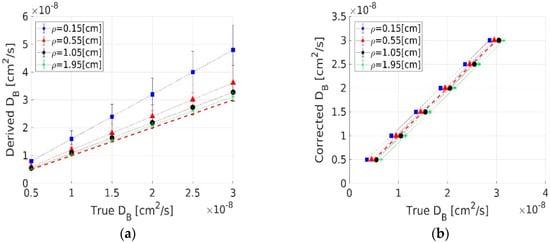
Figure 8.
Estimated Brownian flow coefficients vs. simulated values. (a) shows the coefficients obtained directly by fitting simulated data, where each line shows data for different SDS. Symbols were average values obtained from 35 simulated media having fixed (but changing optical properties); errorbars show standard deviations. (b) shows the same data in (a) after appropriate scaling by correction factors (see text). The errorbars in (b) are smaller than the size of symbols shown and different lines (for different SDS) are shown staggered only for clarity. The dashed line in Figure 8a,b shows .
3.2. Diffusion-Theory Based Analysis of Experiments
3.2.1. Flow Models for Fitting Experimental Data
As described above, experimental phantoms included a flow channel with the fluid in the channel being either actively pumped (flow phantoms –) or with pump turned off (flow phantom ) and were designed to examine the impact of flow dynamics on DCS measurements. However, theoretical fits to these data could be obtained by using the Brownian flow model (, the random flow model () or the shear-flow model ().
Figure 9a,b show theoretical fits (lines) to an experimental acquisition of (symbols) when the pump was switched off (phantom Figure 9a) and when pump flow rate was 5.76 mL/hr (phantom , Figure 9b). Theoretical fits for the three different flow models used are shown by lines (dash-dotted: Brownian flow; solid: random flow; dashed: shear flow). As seen visually (and by residuals in figure legends), the fits to data are poor for the random flow model in Figure 9a and for the Brownian flow model in Figure 9b, while they are excellent for the random flow model in Figure 9b and for the Brownian flow model in Figure 9a. Given that experimentally measured had markedly different decay profiles (by design) in these two phantoms, the results are as anticipated. The shear-flow fit was however able to fit both experimental flow profiles with (0.01) and all experimental data presented below were analyzed using the shear-flow model. This fitting process yielded flow coefficients and , corresponding to the diffusive and the bulk flow components, respectively, for each phantom.
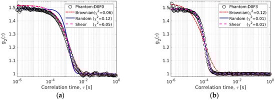
Figure 9.
Experimental data (symbols) and fits using Equation (2) for three different flow models (dash-dotted: Brownian; solid: Random; dashed: shear) for two different flow phantoms. (a) shows representative data in phantom (pump flow turned off) while (b) shows data from phantom (highest pump flow).
3.2.2. Absolute vs. Relative Flow-Coefficients in Phantoms
Figure 10a shows extracted coefficients in phantoms vs. the experimentally controlled pump flow rate. Each symbol-line shows data at fixed channel depth (squares: depth ; triangles: depth ; circles: depth ; asterisks: depth ). The derived Brownian flow coefficients decreased with increasing flow rates, when the flow channel depth was shallowest, while it increased with increasing flow, as the height of the liquid surface above the flow channel was raised. Figure 10b shows the extracted speed of the moving particles from phantoms vs. changing fluid flow speed in the channel. Each symbol-line shows data for fixed channel depth (as in Figure 10a). The pump-flow rate, shown in Figure 10a was converted to a fluid flow speed in the channel (as described in Section 2.1.3) using , where was area of a tube with diameter equal to the inner diameter of the flow channel (0.16 cm). The derived speed of moving particles on the other hand increased with increasing fluid flow speed for the shallow channel depths (squares and triangles in Figure 10b). However, the derived flow speed did not increase linearly with pump flow rate in phantoms with deeper channels (circles and asterisks in Figure 10b).
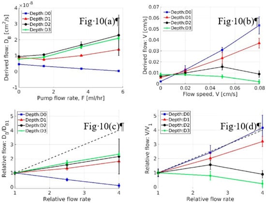
Figure 10.
Derived flow coefficients obtained from fitting phantom data using Equation (2). (a,b) show the retrieved Brownian diffusion and flow speed , for each phantom. Each line shows fixed channel depth (shown in legend), symbols show mean values and error bars are standard deviations (across the five DCS scans obtained for each phantom). (c,d) show relative changes flow vs. relative change in input flow rates, normalized relative to flow phantoms . Dashed line in (c,d) show .
Since the fluid flow in the channel was well-controlled experimentally, we examined relative changes in flow coefficients in the phantoms with actively pumped flow (i.e., across –). Relative flow rates in experiments were calculated as ratio of the pump flow rates of and corresponding to relative flow rates of 2.5 and 4, respectively. Relative changes in phantoms (at each channel depth) were calculated by dividing derived flow coefficients by the flow coefficients obtained for phantoms at pump flow . These data are shown in Figure 10c (for the Brownian flow coefficient ratios) and in Figure 10d (for the shear-flow speed coefficient ratios). Figure 10c,d only show three flow speeds (at each depth) as it does not include data from phantoms when the pump was inactive.
3.3. Simulating Experimental Data Using MC
DCS measurements made on the experimental phantoms were modeled using MC simulations and required input coefficients to describe the phantom model (as described in Section 2.3). These modeling results are presented as two separate cases below, corresponding to phantoms with active flow (pump turned on) and those with inactive flow (pump turned off). In both these cases, the optical transport coefficients and refractive indices for all layers in the tissue model were set to optical coefficients and refractive index of the liquid phantom used, the thickness of layer 2 was matched to the flow channel diameter, and thickness of layer 3 was set to 5 cm (as noted in Table 1). Four input coefficients needed to be determined for simulating each MC phantom tissue model: the height of the liquid layer above the flow channel, and the three flow coefficients for each of the three phantom tissue model layers.
3.3.1. Modeling Phantoms with Inactive Flow
The correlation transport coefficients in each layer of the simulated phantoms when the pump was inactive (i.e., for flow phantoms), were treated as identical across layers and were each set to the same Brownian flow coefficient . Since the fluid in the channel was identical to the liquid media above it, the three-layer model in this case was equivalent to a semi-infinite medium and used = 0. The input value of to the MC phantom tissue model was derived by correcting the Brownian flow coefficient obtained from theoretical fitting—i.e., the retrieved from experimental fits was first multiplied by 0.83 (the correction factor) and then used as input to the MC model. This correction factor was obtained from previously run semi-infinite MC simulations (described in Section 3.1.5 and Figure 7), at the optical transport coefficients of the liquid phantom ( = 0.075/cm and = 12/cm), at the experimentally employed SDS (0.15 cm).
Since variations were observed in coefficients across phantoms , (as seen in Figure 10a), the input Brownian coefficients for MC phantom models simulating different channel depths were obtained by correcting from experimentally fitted data from each phantom at , at each channel depth. Thus, the coefficient obtained from the four phantoms were each multiplied by 0.83 to create input values to MC simulations (since phantoms had same optical properties and were measured at fixed SDS, they had the same correction factor). Figure 11a–d show representative data measured in phantoms (symbols), the corresponding theoretically Brownian flow model fitted using Equation (2) (dashed line), and predicted using MC simulations (solid line), for phantoms , respectively. It is worth noting that the theoretical lines were obtained by fitting the measured data, while the MC data were directly computed (for given inputs). Table 2 lists the values of the input coefficients used in these simulations.
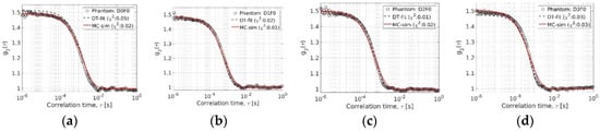
Figure 11.
DCS measurements (symbols) for phantoms , (a–d, respectively) with theoretical fits using a Brownian-flow model (dashed line) and MC predictions (solid line). Each MC model used input values obtained from scaling the theoretically fitted values (see text).
Table 2.
Input coefficients for MC flow phantom models. was constrained to be 0.03 cm experimentally while the relative change in fluid flow speed from flow rate of to was 2.5 (change from to was 4).
3.3.2. Modeling Phantoms with Actively Pumped Flow
As described above, measurements from phantoms were obtaining by changing both the depth of the flow channel and the fluid flow rate in the channel. There were thus 12 phantoms with actively pumped fluid flow—they are identified individually by a combining a flow rate (–), with the channel depth (–). In order to simulate measurements using MC models in these phantoms, inputs for the thickness of Layer 1 (height of the liquid layer , above the flow channel) and flow coefficients for the three layers were needed. For active pumping, correlation transport in Layer 2 (the flow channel) was modeled as random flow, while in Layers 1 and 3 (the liquid media above and below the flow channel, respectively) it was modeled as Brownian, with both layers having the same . These input values were obtained, for each depth, from corresponding MC models shown in Figure 11 (i.e., from phantoms with no active flow).
Input values for two remaining parameters—the depth of the flow channel from surface and the flow speed of the medium in the flow channel—had to be determined. Across 12 phantoms with active flow, relative changes (in both these parameters) were experimentally well controlled. Increases in channel depth (from one depth to the next) was experimentally estimated to approximately be = 0.03 cm. Therefore, if the phantoms at depth had Layer 1 thickness of , then Layer 1 thickness for phantoms with flow channel at depth would be (and further as and ). Similarly, changes in flow speeds could be calculated from experimentally used flow rates—i.e., if the input flow speed was known for phantoms with flow , the flow speeds for flow and would scale as and .
Input values for and were sought by running a set of simulations that varied (between 0–0.05 cm) and (between 0.04 and 0.001 cm/s) to find values that matched experimental measurements for phantom with lowest residuals. From these set of initial simulations, the tissue model with = 0.02 cm and = 5.7 × 10⁻³ cm/s, produced the lowest residuals relative to experimental data acquired in phantom D0F1. Once and were known, required inputs for all 12 tissue models (, and ) were generated by scaling them across phantoms. The (scaled) input values of the coefficients (sought as inputs) for all the 3-layered tissue models constructed are shown in in Table 2.
Figure 12 shows comparisons of experimental measurements (symbols), diffusion theory fits with shear-flow model (dashed black lines) and the MC simulations (solid lines) for one representative measurement, for each of the 12 phantoms with active flow. Data in Figure 12 are organized such that moving across a row, changes channel depth (: Column 1; : Column 2; : Column 3; : Column 4) while moving down a column changes channel flow rate (: Row 1; : Row 2; : Row 3). As seen in Figure 11, the data generated by the MC simulations matched experimental measurements as well as the fitted theoretical curves ( residuals are shown in each figure). Thus, the MC tissue model used could accurately represent the experimental phantom system used.
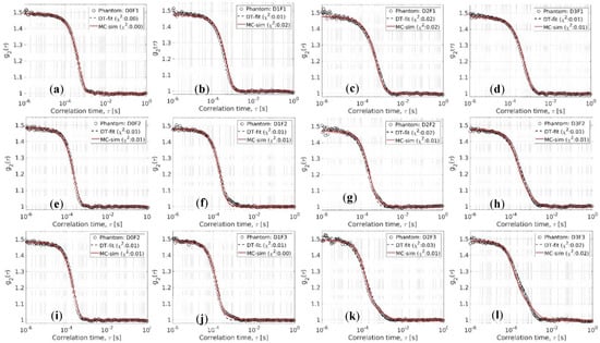
Figure 12.
Comparisons of experimentally measured data (circles), diffusion theory-based fits (dashed line) and MC predictions (solid line) for the 12 phantoms with actively pumped. (a–d) show these data when flow rate was = 1.44 mL/h for depths –. ((e–h) show the same sequence of depths at flow rate = 3.6 mL/h and (i–l) for flow rate = 5.76 mL/h).
4. Discussion
We examine the quantitative impact of analyzing experimental DCS measurements made at short SDS using Equation (2), for different phantoms (with varying optical transport and flow properties) and use MC simulations to directly compare theoretical calculations across range of SDS. Simulations showed expected behavior, where long SDS DCS data well matched and short SDS data being poorly matched for direct, forward comparisons to calculations from Equation (2) Figure 2. However, DCS data obtained at short SDS were well fit using theory at the cost of errors in extracted flow coefficients Figure 3 and Figure 4. Relative changes in perfusion could still be quantified exactly using theory, even for SDS < 0.1 cm Figure 5 and Figure 6. as long as the optical properties of the media considered were not changing. MC simulations were shown to be accurate for calibrating and correcting theoretically retrieved coefficients, given the SDS and optical properties of the medium Figure 7 and Figure 8.
Equation (2) could also directly be used to examine changes in flow in phantoms but required that flow dynamics include both Brownian and Random flow components Figure 9. As shown in Figure 10a,b, extracted both the diffusive flow and random flow coefficients extracted from theoretical analyses of experimental data (at SDS of 0.15 cm) increased with experimentally increasing flow rates. However, the Brownian flow component changed proportionally with flow rate only when the flow channel was submerged deeper below the surface (estimated to be more than 500 μm here). While, for shallower channel depths the flow speed linearly changed with experimentally controlled flow speed. Relative changes in extracted flow coefficients in phantom experiments when flow was actively pumped showed that the ratios of theoretically extracted flow speeds were almost exactly as expected experimentally, but only when the channel depth was shallowest Figure 10d.
These results taken together with relative flow changes extracted in MC simulations for semi-infinite media Figure 8, indicate that theoretical analysis of DCS measurements using Equation (2) is robust and can be used to quantitatively assess changes of relative flow within turbid media, even at short SDS as long as the optical properties and SDS do not change. These conclusions are in accordance with previous findings regarding the accuracy absolute flow rates vs. relative flow at longer SDS [13,16,53]. Our results support findings from recent studies, where Equation (2) was successfully used to examine relative changes in DCS flow coefficients from both simulations and in vivo studies in animal models, at short SDS [27,28,30,31]. However, our findings also indicate that quantification of relative perfusion changes reported by these studies would be estimated more accurately, if the relative changes in perfusion at the short SDS channels were computed with MC-derived correction factors with corresponding changes in media optical properties they measured.
We were also able to predict experimental measurements with MC simulations across all phantoms used Figure 11 and Figure 12. These data showed excellent fits in all phantoms ( 0.03). Given that inputs to tissue models and experiments were tightly coupled and constrained, these data indicate good fidelity of the experimental phantom system used here. Although MC simulations for active flow phantoms matched changes in relative flow rates used experimentally, the absolute value of flow rates (listed in Table 2) were nearly 3.7 times lower than those expected—i.e., the average flow speed in the channel experimentally (given a tube of radius 0.08 cm, and flow rate = 1.56 mL/h) would be = 2.1 × 10⁻² cm/s but the MC inputs for flow speed of in layer 2 was = 5.7 × 10⁻³ cm/s (data in Figure 12b).
There could be a few different reasons for this issue: for e.g., our MC model assumed a flat velocity profile for correlation transport in the channel but a parabolic flow-profile may better physically represent our experimental system; the MC simulations also did not consider flow directions (relative to photon trajectories) in calculations of correlation transport in Equation (3); we also did not investigate simulations in semi-infinite media using random flow models to examine how they were impacted at short SDS. Lastly, the phantom models though were carefully constructed and measured still includes uncertainty about the depth the channel from DCS probe may impact these results. These topics will be examined in future investigations.
Although Equation (2) is widely used to quantify DCS measurements mainly due to its simplicity and ease of use, there have been recent reports that have developed improved theoretical formulations to model DCS measurements directly using correlation transport modeled using the radiative transport theory [54,55]. Such approaches would be better suited for analyzing DCS measurements made at short SDS separations and could be investigated in more detail in the future using the MC simulations and experimental platform presented here.
In summary, we establish that the theoretical expression in Equation (2) used to model DCS measurements of dynamically back scattered reflectance from turbid media can be robust for fitting data obtained experimentally (and numerically) across a wide range of SDS. The parameters obtained from theoretically modeled fits of measurements can be used to quantitatively parametrize relative changes of fluid flow at short SDS only when the optical properties of the media are not changing, across changing flow conditions. Yet, derived flow coefficients using Equation (2) can be linearly corrected to provide absolute flow coefficients, if the optical properties and SDS are known, via MC generated calibration factors. Our findings show that such MC derived correction factors are applicable to DCS measurements that were made at with SDS as small as 0.15 cm.
Author Contributions
Both K.V. and S.Z. contributed to study conceptualization, methodology, investigation, data curation, writing the original draft, visualization. K.V. was responsible for software, writing—review and editing, formal analysis, supervision and validation of data.
Funding
This research received no external funding.
Acknowledgments
We wish to thank Rajan Gurjar for valuable inputs in interpreting and analyzing experimental data and to Louis Gagnon for helpful discussions about approaches for programming correlation transport into our Monte Carlo model. We also acknowledge support from Jens Mueller from the Research Computing Group at Miami for providing guidance with running MC simulations in parallel on the redhawk cluster.
Conflicts of Interest
The authors declare no conflict of interest.
References
- Agochukwu, N.B.; Huang, C.; Zhao, M.; Bahrani, A.A.; Chen, L.; McGrath, P.; Yu, G.; Wong, L. A Novel Noncontact Diffuse Correlation Spectroscopy Device for Assessing Blood Flow in Mastectomy Skin Flaps: A Prospective Study in Patients Undergoing Prosthesis-Based Reconstruction. Plast. Reconstr. Surg. 2017, 140, 26–31. [Google Scholar] [CrossRef]
- Buckley, E.M.; Cook, N.M.; Durduran, T.; Kim, M.N.; Zhou, C.; Choe, R.; Yu, G.; Schultz, S.; Sehgal, C.M.; Licht, D.J.; et al. Cerebral hemodynamics in preterm infants during positional intervention measured with diffuse correlation spectroscopy and transcranial Doppler ultrasound. Opt. Express 2009, 17, 12571. [Google Scholar] [CrossRef]
- Carp, S.A.; Dai, G.P.; Boas, D.A.; Franceschini, M.A.; Kim, Y.R. Validation of diffuse correlation spectroscopy measurements of rodent cerebral blood flow with simultaneous arterial spin labeling MRI; towards MRI-optical continuous cerebral metabolic monitoring. Biomed. Opt. Express 2010, 1, 553–565. [Google Scholar] [CrossRef] [PubMed]
- Han, S.; Hoffman, M.D.; Proctor, A.R.; Vella, J.B.; Mannoh, E.A.; Barber, N.E.; Kim, H.J.; Jung, K.W.; Benoit, D.S.W.; Choe, R. Non-Invasive Monitoring of Temporal and Spatial Blood Flow during Bone Graft Healing Using Diffuse Correlation Spectroscopy. PLoS ONE 2015, 10, e0143891. [Google Scholar] [CrossRef]
- Durduran, T.; Yu, G.; Burnett, M.G.; Detre, J.A.; Greenberg, J.H.; Wang, J.; Zhou, C.; Yodh, A.G. Diffuse optical measurement of blood flow, blood oxygenation, and metabolism in a human brain during sensorimotor cortex activation. Opt. Lett. 2004, 29, 1766–1768. [Google Scholar] [CrossRef] [PubMed]
- Varma, H.M.; Valdés, C.P.; Kristoffersen, A.K.; Culver, J.P.; Durduran, T. Speckle contrast optical tomography: A new method for deep tissue three-dimensional tomography of blood flow. Biomed. Opt. Express 2014, 5, 1275–1289. [Google Scholar] [CrossRef]
- Ramirez, G.; Proctor, A.R.; Jung, K.W.; Wu, T.T.; Han, S.; Adams, R.R.; Ren, J.; Byun, D.K.; Madden, K.S.; Brown, E.B.; et al. Chemotherapeutic drug-specific alteration of microvascular blood flow in murine breast cancer as measured by diffuse correlation spectroscopy. Biomed. Opt. Express 2016, 7, 3610–3630. [Google Scholar] [CrossRef] [PubMed]
- Shang, Y.; Symons, T.B.; Durduran, T.; Yodh, A.G.; Yu, G. Effects of muscle fiber motion on diffuse correlation spectroscopy blood flow measurements during exercise. Biomed. Opt. Express 2010, 1, 500–511. [Google Scholar] [CrossRef]
- Weingarten, M.S.; Papazoglou, E.S.; Zubkov, L.; Zhu, L.; Neidrauer, M.; Savir, G.; Peace, K.; Newby, J.G.; Pourrezaei, K. Correlation of near infrared absorption and diffuse reflectance spectroscopy scattering with tissue neovascularization and collagen concentration in a diabetic rat wound healing model. Wound Repair Regen. 2008, 16, 234–242. [Google Scholar] [CrossRef]
- Yazdi, H.S.; O’Sullivan, T.D.; Leproux, A.; Hill, B.; Durkin, A.; Telep, S.; Lam, J.; Yazdi, S.S.; Police, A.M.; Carroll, R.M.; et al. Mapping breast cancer blood flow index, composition, and metabolism in a human subject using combined diffuse optical spectroscopic imaging and diffuse correlation spectroscopy. J. Biomed. Opt. 2017, 22, 045003. [Google Scholar] [CrossRef]
- Yu, G. Near-infrared diffuse correlation spectroscopy in cancer diagnosis and therapy monitoring. J. Biomed. Opt. 2012, 17, 10901. [Google Scholar] [CrossRef]
- Thong, P.; Lee, K.; Toh, H.J.; Dong, J.; Tee, C.S.; Low, K.P.; Chang, P.H.; Bhuvaneswari, R.; Tan, N.C.; Soo, K.C. Early assessment of tumor response to photodynamic therapy using combined diffuse optical and diffuse correlation spectroscopy to predict treatment outcome. Oncotarget 2017, 8, 19902–19913. [Google Scholar] [CrossRef]
- Shang, Y.; Li, T.; Yu, G. Clinical Applications of Near-infrared Diffuse Correlation Spectroscopy and Tomography for Tissue Blood Flow Monitoring and Imaging. Physiol. Meas. 2017, 38, R1–R26. [Google Scholar] [CrossRef]
- Boas, D.A.; Campbell, L.E.; Yodh, A.G. Scattering and Imaging with Diffusing Temporal Field Correlations. Phys. Rev. Lett. 1995, 75, 1855–1858. [Google Scholar] [CrossRef]
- Boas, D.A.; Yodh, A.G. Spatially varying dynamical properties of turbid media probed with diffusing temporal light correlation. J. Opt. Soc. Am. A 1997, 14, 192. [Google Scholar] [CrossRef]
- Durduran, T.; Choe, R.; Baker, W.B.; Yodh, A.G. Diffuse Optics for Tissue Monitoring and Tomography. Rep. Prog. Phys. 2010, 73, 76701. [Google Scholar] [CrossRef]
- Durduran, T.; Yodh, A.G. Diffuse correlation spectroscopy for non-invasive, micro-vascular cerebral blood flow measurement. Neuroimage 2014, 85, 51–63. [Google Scholar] [CrossRef]
- Cheung, C.; Culver, J.P.; Takahashi, K.; Greenberg, J.H.; Yodh, A.G. In vivo cerebrovascular measurement combining diffuse near-infrared absorption and correlation spectroscopies. Phys. Med. Biol. 2001, 46, 2053–2065. [Google Scholar] [CrossRef]
- Carp, S.A.; Roche-Labarbe, N.; Franceschini, M.A.; Srinivasan, V.J.; Sakadžić, S.; Boas, D.A. Due to intravascular multiple sequential scattering, Diffuse Correlation Spectroscopy of tissue primarily measures relative red blood cell motion within vessels. Biomed. Opt. Express 2011, 2, 2047–2054. [Google Scholar] [CrossRef]
- Chandran, R.S.; Devaraj, G.; Kanhirodan, R.; Roy, D.; Vasu, R.M. Detection and estimation of liquid flow through a pipe in a tissue-like object with ultrasound-assisted diffuse correlation spectroscopy. J. Opt. Soc. Am. A 2015, 32, 1888–1897. [Google Scholar] [CrossRef]
- Farrell, T.J.; Patterson, M.S.; Wilson, B.C. A diffusion theory model of spatially resolved, steady-state diffuse reflectance for the noninvasive determination of the tissue optical properties in vivo. Med. Phys. 1992, 19, 879–888. [Google Scholar] [CrossRef]
- Kaplan, P.D.; Kao, M.H.; Yodh, A.G.; Pine, D.J. Geometric constraints for the design of diffusing-wave spectroscopy experiments. Appl. Opt. 1993, 32, 3828. [Google Scholar] [CrossRef]
- Durian, D.; Rudnick, J. Photon migration at short times and distances and in cases of strong absorption. J. Opt. Soc. Am. A 1997, 14, 235. [Google Scholar] [CrossRef]
- Venugopalan, V.; You, J.S.; Tromberg, B.J. Radiative transport in the diffusion approximation: An extension for highly absorbing media and small source-detector separations. Phys. Rev. E 1998, 58, 2395–2407. [Google Scholar] [CrossRef]
- Yoon, G.; Prahl, S.A.; Welch, A.J. Accuracies in the diffusion approximation and its similarity relations for laser irradiated biological media. Appl. Opt. 1989, 28, 2250–2255. [Google Scholar] [CrossRef]
- Kienle, A.; Patterson, M.S. Improved solutions of the steady-state and the time-resolved diffusion equations for reflectance from a semi-infinite turbid medium. J. Opt. Soc. Am. A 1997, 14, 246. [Google Scholar] [CrossRef]
- Buckley, E.M.; Miller, B.F.; Golinski, J.M.; Sadeghian, H.; McAllister, L.M.; Vangel, M.; Ayata, C.; Meehan, W.P., 3rd; Franceschini, M.A.; Whalen, M.J. Decreased microvascular cerebral blood flow assessed by diffuse correlation spectroscopy after repetitive concussions in mice. J. Cereb. Blood Flow Metab. 2015, 35, 1995–2000. [Google Scholar] [CrossRef]
- Farzam, P.; Durduran, T. Multidistance diffuse correlation spectroscopy for simultaneous estimation of blood flow index and optical properties. J. Biomed. Opt. 2015, 20, 55001. [Google Scholar] [CrossRef]
- Johansson, J.D.; Mireles, M.; Morales-Dalmau, J.; Farzam, P.; Martínez-Lozano, M.; Casanovas, O.; Durduran, T. Scanning, non-contact, hybrid broadband diffuse optical spectroscopy and diffuse correlation spectroscopy system. Biomed. Opt. Express 2016, 7, 481–498. [Google Scholar] [CrossRef]
- Vishwanath, K.; Gurjar, R.; Wolf, D.; Riccardi, S.; Duggan, M.; King, D. Diffuse optical monitoring of peripheral tissues during uncontrolled internal hemorrhage in a porcine model. Biomed. Opt. Express 2018, 9, 569–580. [Google Scholar] [CrossRef]
- Sathialingam, E.; Lee, S.Y.; Sanders, B.; Park, J.; McCracken, C.E.; Bryan, L.; Buckley, E.M. Small separation diffuse correlation spectroscopy for measurement of cerebral blood flow in rodents. Biomed. Opt. Express 2018, 9, 5719–5734. [Google Scholar] [CrossRef]
- Zhu, C.; Liu, Q. Review of Monte Carlo modeling of light transport in tissues. J. Biomed. Opt. 2013, 18, 50902. [Google Scholar] [CrossRef]
- Bender, J.E.; Vishwanath, K.; Moore, L.K.; Brown, J.Q.; Chang, V.; Palmer, G.M.; Ramanujam, N. A Robust Monte Carlo Model for the Extraction of Biological Absorption and Scattering in Vivo. IEEE Trans. Biomed. Eng. 2009, 56, 960–968. [Google Scholar] [CrossRef]
- Zhu, C.; Palmer, G.M.; Breslin, T.M.; Harter, J.; Ramanujam, N. Diagnosis of breast cancer using diffuse reflectance spectroscopy: Comparison of a Monte Carlo versus partial least squares analysis based feature extraction technique. Lasers Surg. Med. 2006, 38, 714–724. [Google Scholar] [CrossRef]
- Palmer, G.M.; Ramanujam, N. Monte Carlo-based inverse model for calculating tissue optical properties Part I: Theory and validation on synthetic phantoms. Appl. Opt. 2006, 45, 1062. [Google Scholar] [CrossRef]
- Swartling, J.; Dam, J.S.; Andersson-Engels, S. Comparison of spatially and temporally resolved diffuse-reflectance measurement systems for determination of biomedical optical properties. Appl. Opt. 2003, 42, 4612. [Google Scholar] [CrossRef]
- Boas, D.A.; Culver, J.P.; Stott, J.J.; Dunn, A.K. Three dimensional Monte Carlo code for photon migration through complex hetrogeneous media including the adult human head. Opt. Express 2002, 10, 159–170. [Google Scholar] [CrossRef]
- Binzoni, T.; Martelli, F. Assessing the reliability of diffuse correlation spectroscopy models on noise-free analytical Monte Carlo data. Appl. Opt. 2015, 54, 5320–5326. [Google Scholar] [CrossRef]
- Boas, D.A.; Sakadžić, S.; Selb, J.; Farzam, P.; Franceschini, M.A.; Carp, S.A. Establishing the diffuse correlation spectroscopy signal relationship with blood flow. Neurophotonics 2016, 3, 31412. [Google Scholar] [CrossRef]
- Gagnon, L.; Desjardins, M.; Jehanne-Lacasse, J.; Bherer, L.; Lesage, F. Investigation of diffuse correlation spectroscopy in multi-layered media including the human head. Opt. Express 2008, 16, 15514. [Google Scholar] [CrossRef]
- Selb, J.; Boas, D.A.; Chan, S.T.; Evans, K.C.; Buckley, E.M.; Carp, S.A. Sensitivity of near-infrared spectroscopy and diffuse correlation spectroscopy to brain hemodynamics: Simulations and experimental findings during hypercapnia. Neurophotonics 2014, 1, 15005. [Google Scholar] [CrossRef]
- Binzoni, T.; Liemert, A.; Kienle, A.; Martelli, F. Analytical solution of the correlation transport equation with static background: Beyond diffuse correlation spectroscopy. Appl. Opt. 2016, 55, 8500. [Google Scholar] [CrossRef]
- Vishwanath, K.; Chang, K.; Klein, D.; Deng, Y.F.; Chang, V.; Phelps, J.E.; Ramanujam, N. Portable, Fiber-Based, Diffuse Reflection Spectroscopy (DRS) Systems for Estimating Tissue Optical Properties. Appl. Spectrosc. 2011, 65, 206–215. [Google Scholar] [CrossRef]
- Wu, H.I.; Wang, L.V. Raleigh theory and Mie theory for single scatterer. In Biomedical Opticsl Priniciples and Imaging; John Wiley & Sons: Hobken, NJ, USA, 2007. [Google Scholar]
- Taroni, P.; Pifferi, A.; Torricelli, A.; Comelli, D.; Cubeddu, R. In vivo absorption and scattering spectroscopy of biological tissues. Photochem. Photobiol. Sci. 2003, 2, 124–129. [Google Scholar] [CrossRef]
- Barman, I.; Dingari, N.C.; Rajaram, N.; Tunnell, J.W.; Dasari, R.R.; Feld, M.S. Rapid and accurate determination of tissue optical properties using least-squares support vector machines. Biomed. Opt. Express 2011, 2, 592–599. [Google Scholar] [CrossRef]
- Honda, N.; Ishii, K.; Terada, T.; Nanjo, T.; Awazu, K. Determination of the tumor tissue optical properties during and after photodynamic therapy using inverse Monte Carlo method and double integrating sphere between 350 and 1000 nm. J. Biomed. Opt. 2011, 16, 58003. [Google Scholar] [CrossRef]
- Ivanov, K.; Kalinina, M.; Levkovich, Y. Blood flow velocity in capillaries of brain and muscles and its physiological significance. Microvasc. Res. 1981, 22, 143–155. [Google Scholar] [CrossRef]
- Vishwanath, K.; Mycek, M.A. Time-resolved photon migration in bi-layered tissue models. Opt. Express 2005, 13, 7466. [Google Scholar] [CrossRef]
- Wang, L.; Jacques, S.L.; Zheng, L. MCML–Monte Carlo modeling of photon transport in multi-layered tissues. Comput. Methods Programs Biomed. 1995, 47, 131–146. [Google Scholar] [CrossRef]
- Vishwanath, K.; Pogue, B.; Mycek, M.-A. Quantitative fluorescence lifetime spectroscopy in turbid media: Comparison of theoretical, experimental and computational methods. Phys. Med. Biol. 2002, 47, 3387–3405. [Google Scholar] [CrossRef]
- Wu, X.L.; Pine, D.J.; Chaikin, P.M.; Huang, J.S.; Weitz, D.A. Diffusing-wave spectroscopy in a shear flow. J. Opt. Soc. Am. B 1990, 7, 15–20. [Google Scholar] [CrossRef]
- Shang, Y.; Gurley, K.; Yu, G. Diffuse Correlation Spectroscopy (DCS) for Assessment of Tissue Blood Flow in Skeletal Muscle: Recent Progress. Anat. Physiol. 2013, 3, 128. [Google Scholar]
- Binzoni, T.; Liemert, A.; Kienle, A.; Martelli, F. Derivation of the correlation diffusion equation with static background and analytical solutions. Appl. Opt. 2017, 56, 795. [Google Scholar] [CrossRef]
- Binzoni, T.; Sanguinetti, B.; Van De Ville, D.; Zbinden, H.; Martelli, F. Probability density function of the electric field in diffuse correlation spectroscopy of human bone in vivo. Appl. Opt. 2016, 55, 757–762. [Google Scholar] [CrossRef]


© 2019 by the authors. Licensee MDPI, Basel, Switzerland. This article is an open access article distributed under the terms and conditions of the Creative Commons Attribution (CC BY) license (http://creativecommons.org/licenses/by/4.0/).