Abstract
Three-dimensional printing quality is critically affected by the transmission condition of 3D printers. A low-cost technique based on the echo state network (ESN) is proposed for transmission condition monitoring of 3D printers. A low-cost attitude sensor installed on a 3D printer was first employed to collect transmission condition monitoring data. To solve the high-dimensional problem of attitude data, feature extraction approaches were subsequently performed. Based on the extracted features, the ESN was finally employed to monitor transmission faults of the 3D printer. Experimental results showed that the fault recognition accuracy of the 3D printer was obtained at 97.17% using the proposed approach. In addition, support vector machine (SVM), locality preserving projection support vector machine (LPPSVM), and principal component analysis support vector machine (PCASVM) were also used for comparison. The contrast results showed that the recognition accuracies of our method were higher and more stable than that of SVM, LPPSVM, and PCASVM when collecting raw data via the low-cost attitude sensor.
1. Introduction
As a rapid prototyping technology, 3D printing is based on a digital model and can be sticky with powdered metal or plastic. Materials are used to construct objects via layer-by-layer printing [1]. The application domain of 3D printing is expanding rapidly. In the electronics, aviation, automobile manufacturing, and medical industries, 3D printing can produce small batches of customized components with low cost and high efficiency [2]. The quality of 3D printing products are greatly reduced when transmission faults occur [3]. Under these circumstances, a novel cable-driven parallel 3D printer was developed to fine tune the transmission of 3D printers [4], and a spring-assisted mechanism was investigated to identify the transmission performance of 3D printers by comparison with a conventional tilting mechanism [5]. However, even if the transmission mechanism of the 3D printer is well designed, it will encounter faults during its life time. In summary, it is necessary to develop low-cost transmission condition monitoring techniques for 3D printers, which will monitor the quality of 3D printing.
Over the past few decades, many methods for monitoring mechanical systems have been developed, such as vibration monitoring, temperature-based diagnosis, spectrum analysis, etc. [6,7]. For instance, condition monitoring of machine-bearing housing using the measured experimental values of the acceleration amplitude of mechanical vibrations was studied in Reference [8], a new switching unscented Kalman filter algorithm was proposed in Reference [9] to predict the remaining useful life of bearings, and a method based on a generalized synchro-squeezing transform with vibration data was proposed to detect gearbox faults in Reference [10]. In addition, work in condition monitoring for machinery includes an approach using moment and rotor angle sensors that was proposed to monitor wind turbines [11] and the use of multiple sparse auto-encoders reported for dynamic state monitoring of 3D printers [12]. At present, new intelligent classification methods such as artificial neural networks (ANNs) [13], SVM [14], fuzzy logic [15], and neighborhood preserving embedding (NPE) [16] have been gradually employed for condition monitoring.
An ANN is an information processing system designed to imitate the way human brain’s work [17]. This model has the capabilities of associative memory, pattern matching, and similarity induction. This is why the model has the ability to accomplish nonlinear mapping the relationship between system states and fault causes [18]. However, ANN tends to fall into local minimum and over-fitting problems when applied to condition monitoring [19]. In Reference [20], it was confirmed that a back propagation neural network (BPNN), a kind of ANN, is not an effective technique for condition monitoring of 3D printers, while SVMs can effectively diagnose 3D printers when using high-cost attitude sensors. However, data noise increases when low-cost attitude sensors are employed for data collection. Thus, the condition monitoring accuracy of SVMs will decrease dramatically. For this reason, it is necessary to propose a more effective monitoring method for 3D printers.
The echo state network (ESN), proposed by Jaeger in 2001 [21], is a type of recurrent neural network, which includes a large, sparse, and randomly connected set of neurons, known as the reservoir. After initialization, the reservoir remains fixed and the learning effort is only necessary for the output (readout) connections. The ESN can be viewed as a type of reservoir computing (RC) and is particularly suitable for time-series processing [22]. In this paper, the monitoring data of the 3D printer was time-series data. Moreover, the ESN is still an effective method in dealing with time-series data with high noise [21,22,23]. Hence, ESN is employed for transmission condition monitoring of 3D printers in this paper. However, due to the high dimension of the attitude data, it is better to extract some features as the input data for ESN.
Feature extraction refers to constructing some features via mapping the useful information contained in the original feature to a lower dimension feature space [24]. There are many ways to extract features such as data mining techniques, statistical feature extraction techniques, and neural network methods. Traditional feature extraction methods are employed to condition monitoring, including empirical mode decomposition [25], linear discriminant analysis (LDA) [26], and locality preserving projection (LPP) [27]. These feature extraction methods are proven to be effective in improving the accuracy of condition monitoring when data noise is high. For monitoring the 3D printer more effectively, it is necessary to extract features from raw data before ESN modeling. Correspondingly, a technique based on the echo state network is presented in this paper to monitor the transmission system of 3D printers.
2. Methodologies
The details of the proposed method are introduced in this section. The first step is to extract features from the data, which is introduced in Section 2.1. Then, an explanation on how to use the features in the ESN is given in Section 2.2. An overview of the present approach is subsequently provided in Section 2.3.
2.1. Feature Extraction
Due to the high dimension and noise of the time-series data obtained by monitoring the 3D printer, it was very important to extract features from the time-series data. The data from the 3D printer can be extracted in different modalities such as time-domain features and time-frequency features. It should be noted that features in one domain are insufficient to reflect all aspects of the faults. Hence, both time-domain and time-frequency features are applied to fault diagnosis in this work.
To obtain time-domain features from the raw data (i.e., monitoring data), 10 time-domain statistical features including mean, mean square, skewness, kurtosis, peak value, root mean square magnitude, crest factor, waveform factor, clearance factor, and impulse factor were used in this paper, which can reduce noise interference and increase the model’s robustness [28]. These 10 features are described as follows:
Given a set of data yi (i = 1, 2, ..., n), where yi represents the data at the i-th time, the mean of the data can be expressed by Equation (1).
The mean square of the data, which can be calculated via Equation (2), is adopted to eliminate the influence of the time-series data on the sum of squares of errors.
Skewness of the data is used to reflect the degree of asymmetry of distribution, which is expressed in the following equation:
where Ysd represents the standard deviation of the data. The kurtosis shown in Equation (4) is used to characterize the number of peaks of the probability density distribution curve at the average value.
The peak value reflects the range and intensity of the amplitude of the signal. The expression of peak value is defined as follows:
The calculation method of the root mean square magnitude of the data is written in Equation (6).
The crest factor is the ratio of the peak to RMS magnitude, which can be calculated as follows:
The waveform factor is the ratio of RMS to absolute mean, which can be calculated via Equation (8).
The clearance factor and the impulse factor are expressed in Equations (9) and (10), respectively.
where YR is square root amplitude of yi.
The wavelet packet energy is employed as a frequency feature. The expression of wavelet packet energy [29] is written in Equation (11).
where wi (i = 1, 2, ..., 8) is the i-th wavelet packet energy, and W3i means the i-th frequency range of three-level wavelet packets. In this paper, time-frequency features including the eight-wavelet packet energy was considered for monitoring 3D printers. In addition to the 10 time-domain features mentioned above, there are 18 features in total.
2.2. The Concept of ESN
Both the ESN and liquid state machine (LSM) are machine learning methods for time-series analysis, which are collectively referred to as reservoir computing methods [29]. Just as its name implies, the ESN is composed of an input layer, hidden layer (i.e., reservoir), and an output layer. The hidden layer is designed as a sparse network with many neurons. By adjusting the weights of the network, the function of memory data can be achieved. The dynamic reservoir of the network, which contains a large number of sparsely connected neurons, has the advantage of a short training time. The ESN training is only needed to train the connection weights from the hidden layer to the output layer. In this work, the reason for choosing the ESN was because of its more efficient construction and training method.
As shown in Figure 1, there are three distinct sets of neurons including input, the reservoir, and the output layer to construct the ESN. The input, the reservoir, and the output layer contain k, m and L nodes respectively and wout and wback represent output and feedback weight matrices respectively. The weight matrices win and w are initialized randomly when training an ESN model [30].
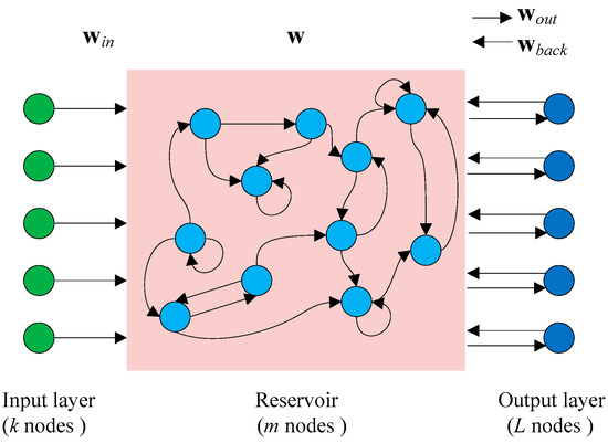
Figure 1.
Schematic of the ESN (Echo State Network).
The state update of the network is governed by two state-space equations, as written in Equations (12) and (13). Firstly, updating the reservoir states at each time step is defined by Equation (12).
where win and w are randomly initialized for a standard normal distribution to ensure that the ESN has properties of an echo state and is fixed at the time when the network was first built. x(t) represents the reservoir states, u(t) denotes network inputs, and f(.) is a predefined activation function. Then the reservoir output is governed by Equation (13).
where z(t) is the reservoir output at a given time step, g(.) represents the output layer neuron activation function, [u(t);x(t)] denotes the extended state vector, and wout is optimized via minimizing the mean square error of z(t).
It is the core fundamental of an ESN that the reservoir is a randomly generated, large-scale, sparse connection, which usually maintains one to five percent of the recursive connections structure. The parameters’ optimization, including spectrum radius (SR), reservoir scale (N), input unit scale (IS), and the sparse degree (SD), is performed to improve the performance of the ESN. The definition of SR is described in Equation (14). Spectrum radius should be satisfied with Equation (15) to ensure reservoir stability.
where λmax represents the parameter of SR, λ(w) is the eigenvalues of connection weight matrices. The parameter N is the number of neurons in the reservoir, which has a great influence on the ESN’s performance. The larger the reservoir is, the more accurate the ESN describes the given dynamic system. However, it may also lead to over-fitting problems. The parameter IS is related to the degree of non-linearity of samples. The parameter SD represents the connection between neurons in the reservoir. The definition of SD is described in Equation (16).
where m represents the number of interconnected neurons, M denotes the total number of neurons. The ESN can improve the performance of non-linear processing when the parameter SD increases.
The training process of the ESN is divided into two stages: samples generation and weight calculation, i.e., the connection weight matrix wout is determined according to the given training samples. Suppose that the training sample (u(t), t = 1, 2, ..., p) is added to the reservoir through the input connection matrix win. The reservoir states x(t) and reservoir output z(t) are sequentially calculated according to Equations (12) and (13), respectively. In the j-th time, matrix B and T can be constituted in Equation (17)
where xm(p) is the state of the m reservoir neurons at the p-th time, and z(p) represents reservoir output at the p-th time. The weight calculation can be performed according to Equation (18) based on the collection of state matrix B and reservoir output T.
where represents predicted reservoir output. The objective function can be expressed in Equation (19) to satisfy the minimum variance of the system.
Correspondingly, it can be reduced using Equation (20).
Therefore, the ESN model can be built according to the aforementioned methods with a simple design and implementation.
2.3. Overview of the Present Approach
According to the previous analysis, the schematic of the present method to monitor the transmission condition of 3D printer is illustrated in Figure 2.
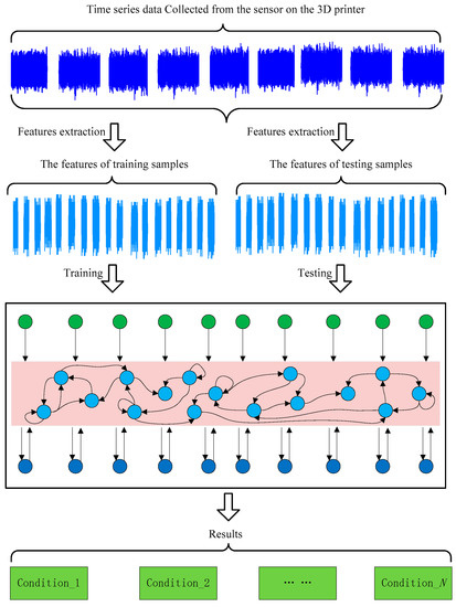
Figure 2.
Schematic of transmission condition monitoring of 3D printers based on ESN.
- Step 1.
- Collect raw monitoring data from the sensor on the 3D printer;
- Step 2.
- Feature extraction from raw monitoring data including ten time-domain statistical features and eight time-frequency features;
- Step 3.
- Train the ESN model using the extracted features;
- Step 4.
- Test the monitoring accuracy of the healthy condition of the 3D printer with the built ESN model; and
- Step 5.
- Output the condition of the 3D printer; end.
3. Experiments
The experiment was carried out to validate the effectiveness of the monitoring method for 3D printers. The experimental configuration included a laptop (Inspiron N4110, DELL, Round Rock, TX, USA), a delta 3D printer (SLD-BL600-6, SHILEIDI, Dongguan, China), and a low-cost attitude sensor (BWT901, WIT, Shenzhen, China), as shown in Figure 3. The price of the employed attitude sensor in this work was approximately $20. The attitude sensor resolutions of acceleration and angular velocity were less than 5.98 × 10⁻⁵ m/sec2 and 7.6 × 10⁻³ deg/sec, respectively. The delta 3D printer based on the prototype principle of fused deposition modeling (FDM) with a symmetrical parallel transmission mechanism was employed with the experiments in this paper. Compared to the series transmission mechanism, the delta 3D printer with a parallel transmission mechanism shows such advantages such as a compact structure, good stiffness and, especially, printing precision. However, printing quality will decrease with the wear and tear of printer parts including joint bearings and synchronous belts in the transmission chain of a 3D printer. Accordingly, an attitude sensor was installed at the end of the delta 3D printer kinematic chain to reflect the printing condition. The low-cost attitude sensor based on a micro electro mechanical system (MEMS) can be made extremely light and compact. Therefore, the printing quality of the 3D printer after installing the attitude sensor will not be affected. The output of the attitude sensor consists of nine channels including three-axial angular velocity signals, three-axial acceleration signals, and three-axial magnetic field intensity signals.
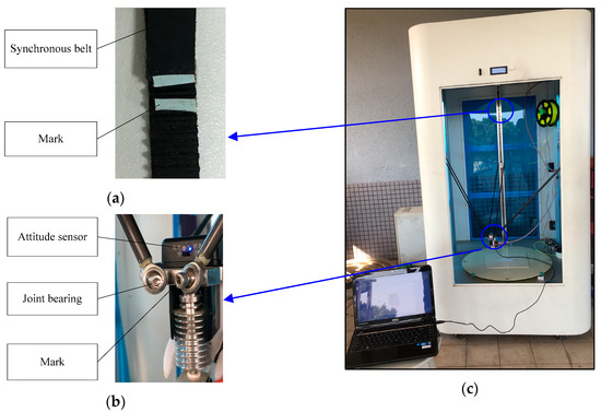
Figure 3.
Experimental configuration: (a) synchronous belt; (b) joint bearing; (c) overview.
There were three major steps in the experiments, as depicted in Figure 4. The first step was to set-up the printing program (i.e., G-code). After building a cylindrical shell model with a radius of 75 mm in SolidWorks (a 3D modeling software), the 3D model of the cylindrical shell was sliced layer by layer via Repetier-Host (a slicing software) to generate G-code. The second step was to collect monitoring data. Due to the parts that are prone to failure in the transmission chain of a delta 3D printer, which include 12 joint bearings and three synchronous belts, the transmission condition of the delta 3D printer was divided into 16 classes, as listed in Table 1. The degree of fault as defined in this work was moderately faulty. When the delta 3D printer executes a printing program under different conditions, the raw monitoring data can be collected with the attitude sensor connected to a laptop. In this work, the frequency of data acquisition by the attitude sensor is set to 100 Hz. Finally, feature extraction for raw monitoring data was performed, including 10 time-domain statistical features and 8 time-frequency features, as introduced in Section 2.1. After the ESN model is built using the aforementioned features, the accuracy of the ESN model can then be obtained through testing.
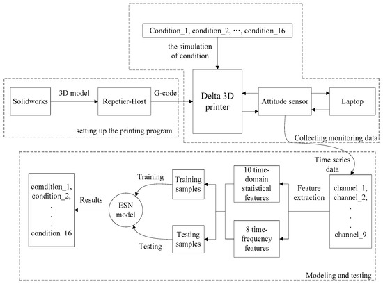
Figure 4.
Experiment flow chart.

Table 1.
Conditions of the delta 3D printer designed in the experiment.
In this work, nine channels of the attitude sensor including three-axial angular velocity signals, three-axial acceleration signals, and three-axial magnetic field intensity signals were employed for sample generation. In the experiment, 60 sets of circular data were collected for each condition and divided into 150 pieces. Moreover, 216 data acquisition points for each channel were obtained and were transformed to 10 time-domain features and 8 frequency-domain features as already described. Therefore, 2400 × 162 samples were collected in total.
4. Results and Discussion
4.1. Experimental Results Using the Proposed Method
The accuracy of the ESN model using different channel data and all nine channels under different proportion training samples is presented in Figure 5. The precision shown in the diagram is the mean of five tests. As can be seen in Figure 5a, the accuracy of the ESN will increase as the proportion of training samples increases. The accuracy of the ESN was 69.82% when only using 7–9 channels of the attitude sensor to generate data and the proportion of training samples was 50%. The monitoring accuracy of the ESN model was almost the same when the data from channels 1–3 and channels 4–6 were employed to train and test the ESN model using the same training sample proportion. The highest accuracy was 87.01% in these three methods to monitor the delta 3D printer. Consequently, the experimental results demonstrate that the choice of data will affect the accuracy of transmission condition monitoring of 3D printers.
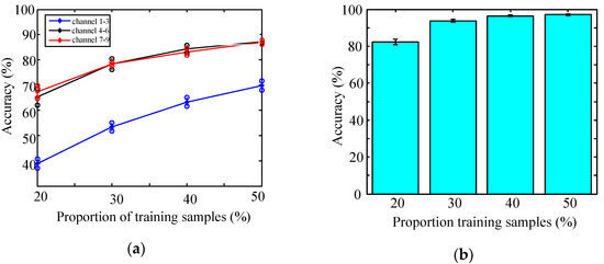
Figure 5.
The accuracy of the proposed method under different proportions of training samples: (a) using different channels’ data and (b) all nine channels’ data.
As depicted in Figure 5b, compared with the method in Figure 5a, a higher monitoring accuracy was obtained when all the channel data of the attitude sensor were used for sample generation. With the enlarged proportion of training samples, the mean increased and the variance decreased. This experimental result indicates that the increase in the training samples’ proportion will improve and stabilize the accuracy of monitoring. The highest accuracy was 97.17%, which was obtained using the proposed method to monitor the delta 3D printer with all nine channels’ data from the attitude sensor. It should be noted that when the proportion of training samples was only 20%, that is only 30 training samples, the accuracy of the ESN model for 3D printer transmission state monitoring was 82.17%. The results identified that the ESN can still guarantee high precision in small samples with low computational resources because the ESN is a shallow learning model.
4.2. Comparison with Peer Methods
As shown in Figure 6, SVM, LPPSVM, and PCASVM were adopted for comparison with the ESN. As can be seen from the bar graph in Figure 6, the monitoring accuracy of SVM, LPPSVM, and PCASVM will not increase when the proportion of training samples increases. The highest accuracy was 48.87% using these three methods to monitor 3D printers. Furthermore, compared to the ESN, the monitoring accuracy of the three methods was not stable.
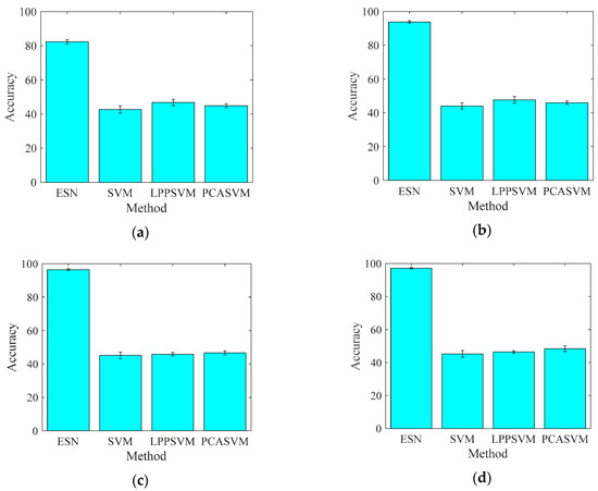
Figure 6.
Accuracy comparison among ESN, SVM, LPPSVM and PCASVM using all nine channels data under (a) 20%, (b) 30%, (c) 40%, and (d) 50% proportion training samples.
5. Conclusions
For economical condition monitoring of 3D printers in practical applications, low-cost signal acquisition and efficient computing methods are necessary. In this paper, a method based on the ESN was proposed to monitor the transmission condition of a 3D printer using a low-cost attitude sensor. Firstly, the fault data of the 3D printer transmission was collected using a simple and low-cost data acquisition system. Then, the ESN model was trained by extracting 10 time-domain statistical features and 8 frequency-domain features using the nine channels’ data from the attitude sensor. The experimental results showed the effectiveness of the proposed method for condition monitoring of 3D printers. The highest monitoring accuracy of this method was 97.17%. It should be pointed out that SVM, LPPSVM, and PCASVM are invalid methods to monitor 3D printers when using the low-cost attitude sensor for data collection as their highest monitoring accuracy was only 48.87%. Compared with SVM, LPPSVM, and PCASVM, the ESN was a highly accurate and stable method for monitoring 3D printers. Therefore, the proposed data-driven method can be used for effective and economical condition monitoring of 3D printers.
Author Contributions
The topic of this research is designed by S.Z. and J.L.; Experiments is performed by K.H. and C.L.; Formal analysis is completed by D.C., C.L. and J.L.; Methodology validation is carried out by S.Z., Y.B. and D.C.; The first version of manuscript is prepared by K.H. and J.L., and this version of the manuscript is read, approved and substantially contributed by all authors.
Funding
This work was supported in part by the National Natural Science Foundation of China (71801046, 51605406 and 51775112), the Research Program of Higher Education of Guangdong (2016KZDXM054), and Postdoctoral Science Foundation of China (2019M652881).
Acknowledgments
We hereby acknowledge that this work was supported by DGUT: Intelligent Manufacturing System Health Monitoring and Maintenance Technology Research Center of Guangdong at Dongguan University of Technology. The valuable comments and suggestions from the editors and the anonymous reviewers are very much appreciated.
Conflicts of Interest
The authors declare no conflict of interest.
References
- Tofail, S.A.M.; Koumoulos, E.P.; Bandyopadhyay, A.; Bose, S.; O’Donoghue, L.; Charitidis, C. Additive manufacturing: Scientific and technological challenges, market uptake and opportunities. Mater. Today 2018, 21, 22–37. [Google Scholar] [CrossRef]
- Rahman, Z.; Ali, S.F.B.; Ozkan, T.; Charoo, N.A.; Reddy, I.K.; Khan, M.A. Additive Manufacturing with 3D Printing: Progress from Bench to Bedside. AAPS J. 2018, 20, 14. [Google Scholar] [CrossRef] [PubMed]
- Bandyopadhyay, A.; Heer, B. Additive manufacturing of multi-material structures. Mater. Sci. Eng. R Rep. 2018, 129, 16. [Google Scholar] [CrossRef]
- Zi, B.; Wang, N.; Qian, S.; Bao, K.L. Design, stiffness analysis and experimental study of a cable-driven parallel 3D printer. Mech. Mach. Theory 2019, 132, 207–222. [Google Scholar] [CrossRef]
- Lin, Y.S.; Yang, C.J. Spring Assisting Mechanism for Enhancing the Separation Performance of Digital Light Process 3D Printers. IEEE Access 2019, 7, 71718–71729. [Google Scholar] [CrossRef]
- Li, C.; Cerrada, M.; Cabrera, D.; Sanchez, R.V.; Pacheco, F.; Ulutagay, G.; de Oliveira, J.V. A comparison of fuzzy clustering algorithms for bearing fault diagnosis. J. Intell. Fuzzy Syst. 2018, 34, 3565–3580. [Google Scholar] [CrossRef]
- Cui, L.L.; Huang, J.F.; Zhang, F.B.; Chu, F.L. HVSRMS localization formula and localization law: Localization diagnosis of a ball bearing outer ring fault. Mech. Syst. Signal Proc. 2019, 120, 608–629. [Google Scholar] [CrossRef]
- Panda, A.; Olejarova, S.; Valicek, J.; Harnicarova, M. Monitoring of the condition of turning machine bearing housing through vibrations. Int. J. Adv. Manuf. Technol. 2018, 97, 401–411. [Google Scholar] [CrossRef]
- Cui, L.L.; Wang, X.; Xu, Y.G.; Jiang, H.; Zhou, J.P. A novel Switching Unscented Kalman Filter method for remaining useful life prediction of rolling bearing. Measurement 2019, 135, 678–684. [Google Scholar] [CrossRef]
- Li, C.; Liang, M. Time-frequency signal analysis for gearbox fault diagnosis using a generalized synchrosqueezing transform. Mech. Syst. Signal Proc. 2012, 26, 205–217. [Google Scholar] [CrossRef]
- Niemann, H.; Poulsen, N.K.; Mirzaei, M.; Henriksen, L.C. Fault diagnosis and condition monitoring of wind turbines. Int. J. Adapt. Control Signal Proc. 2018, 32, 586–613. [Google Scholar] [CrossRef]
- Zhang, S.H.; Sun, Z.Z.; Long, J.Y.; Li, C.; Bai, Y. Dynamic condition monitoring for 3D printers by using error fusion of multiple sparse auto-encoders. Comput. Ind. 2019, 105, 164–176. [Google Scholar] [CrossRef]
- Sadegh, H.; Mehdi, A.N.; Mehdi, A. Classification of acoustic emission signals generated from journal bearing at different lubrication conditions based on wavelet analysis in combination with artificial neural network and genetic algorithm. Tribol. Int. 2016, 95, 426–434. [Google Scholar] [CrossRef]
- Bai, Y.; Sun, Z.Z.; Zeng, B.; Long, J.Y.; Li, L.; de Oliveira, J.V.; Li, C. A comparison of dimension reduction techniques for support vector machine modeling of multi-parameter manufacturing quality prediction. J. Intell. Manuf. 2019, 30, 2245–2256. [Google Scholar] [CrossRef]
- Li, C.; Oliveira, J.L.V.D.; Lozada, M.C.; Cabrera, D.; Sanchez, V.; Zurita, G. A systematic review of fuzzy formalisms for bearing fault diagnosis. IEEE Trans. Fuzzy Syst. 2018. [Google Scholar] [CrossRef]
- Zhang, S.; Sun, Z.; Wang, M.; Long, J.; Bai, Y.; Li, C. Deep Fuzzy Echo State Networks for Machinery Fault Diagnosis. IEEE Trans. Fuzzy Syst. 2019. [Google Scholar] [CrossRef]
- Jami, A.; Heyns, P.S. Impeller fault detection under variable flow conditions based on three feature extraction methods and artificial neural networks. J. Mech. Sci. Technol. 2018, 32, 4079–4087. [Google Scholar] [CrossRef]
- Raptodimos, Y.; Lazakis, I. Using artificial neural network-self-organising map for data clustering of marine engine condition monitoring applications. Ships Offshore Struct. 2018, 13, 649–656. [Google Scholar] [CrossRef]
- Elangovan, K.; Tamilselvam, Y.K.; Mohan, R.E.; Iwase, M.; Nemoto, T.; Wood, K. Fault Diagnosis of a Reconfigurable Crawling-Rolling Robot Based on Support Vector Machines. Appl. Sci. 2017, 7, 1025. [Google Scholar] [CrossRef]
- He, K.; Yang, Z.J.; Bai, Y.; Long, J.Y.; Li, C. Intelligent Fault Diagnosis of Delta 3D Printers Using Attitude Sensors Based on Support Vector Machines. Sensors 2018, 18, 1298. [Google Scholar] [CrossRef]
- Jaeger, H. The “echo state” approach to analyzing and training recurrent neural network. In German National Research Center for Information Technology GMD Technical Report; German National Research Center: Bonn, Germany, 2001. [Google Scholar]
- Cabrera, D.; Sancho, F.; Cerrada, M.; Sanchez, R.V.; Tobar, F. Echo state network and variational autoencoder for efficient one-class learning on dynamical systems. J. Intell. Fuzzy Syst. 2018, 34, 3799–3809. [Google Scholar] [CrossRef]
- Fink, O.; Zio, E.; Weidmann, U. Fuzzy Classification With Restricted Boltzman Machines and Echo-State Networks for Predicting Potential Railway Door System Failures. IEEE Trans. Reliab. 2015, 64, 861–868. [Google Scholar] [CrossRef]
- Long, J.Y.; Sun, Z.Z.; Pardalos, P.M.; Hong, Y.; Zhang, S.H.; Li, C. A hybrid multi-objective genetic local search algorithm for the prize-collecting vehicle routing problem. Inf. Sci. 2019, 478, 40–61. [Google Scholar] [CrossRef]
- Li, C.; Tao, Y.; Ao, W.G.; Yang, S.; Bai, Y. Improving forecasting accuracy of daily enterprise electricity consumption using a random forest based on ensemble empirical mode decomposition. Energy 2018, 165, 1220–1227. [Google Scholar] [CrossRef]
- Bazdar, A.; Kazemzadeh, R.B.; Niaki, S.T.A. Fault diagnosis within multistage machining processes using linear discriminant analysis: A case study in automotive industry. Qual. Technol. Quant. Manag. 2017, 14, 129–141. [Google Scholar] [CrossRef]
- Tang, X.H.; Wang, J.C.; Lu, J.G.; Liu, G.K.; Chen, J.D. Improving Bearing Fault Diagnosis Using Maximum Information Coefficient Based Feature Selection. Appl. Sci. 2018, 8, 2143. [Google Scholar] [CrossRef]
- Li, C.; Sanchez, R.V.; Zurita, G.; Cerrada, M.; Cabrera, D. Fault Diagnosis for Rotating Machinery Using Vibration Measurement Deep Statistical Feature Learning. Sensors 2016, 16, 895. [Google Scholar] [CrossRef]
- Wootton, A.J.; Butcher, J.B.; Kyriacou, T.; Day, C.R.; Haycock, P.W. Structural health monitoring of a footbridge using Echo State Networks and NARMAX. Eng. Appl. Artif. Intell. 2017, 64, 152–163. [Google Scholar] [CrossRef]
- Xu, M.L.; Han, M.; Lin, H.F. Wavelet-denoising multiple echo state networks for multivariate time series prediction. Inf. Sci. 2018, 465, 439–458. [Google Scholar] [CrossRef]


© 2019 by the authors. Licensee MDPI, Basel, Switzerland. This article is an open access article distributed under the terms and conditions of the Creative Commons Attribution (CC BY) license (http://creativecommons.org/licenses/by/4.0/).