Numerical Study on Thermal Design of a Large-Area Hot Plate with Heating and Cooling Capability for Thermal Nanoimprint Lithography


Abstract
:1. Introduction
2. Model
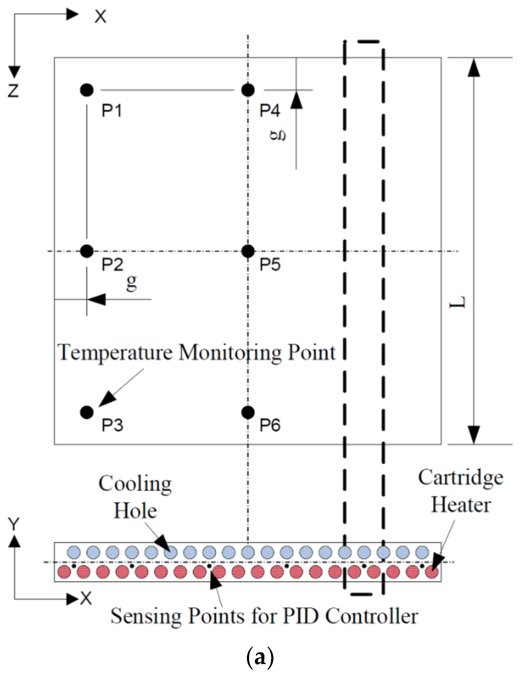
2.1. Physical Model
2.2. Computation Analysis Model
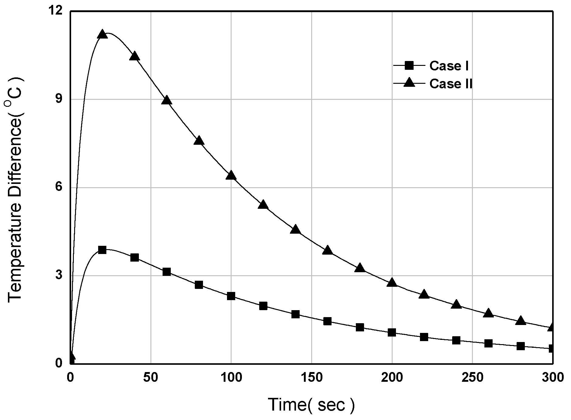
3. Hot Plate Concept Model Comparison Evaluation
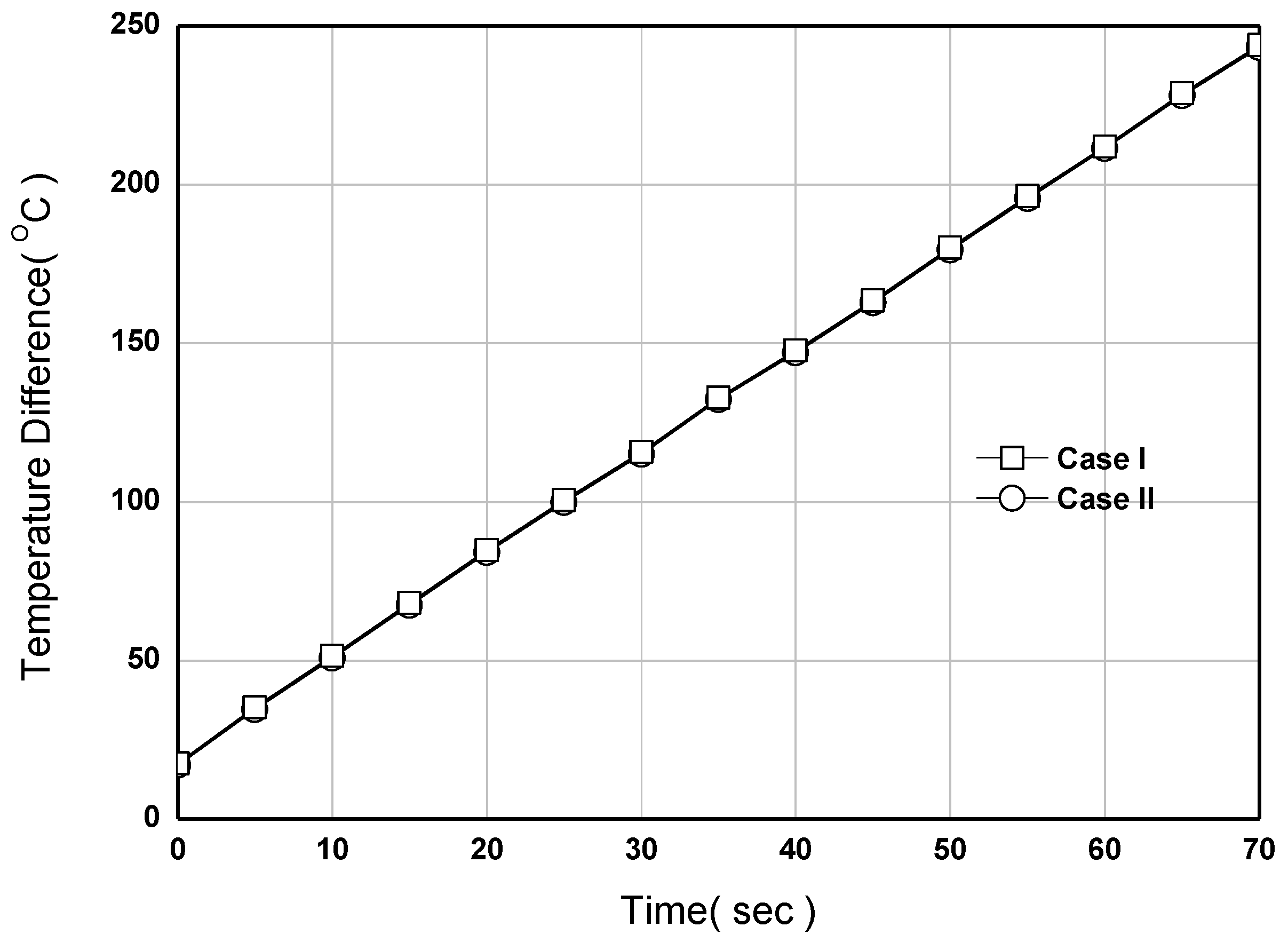
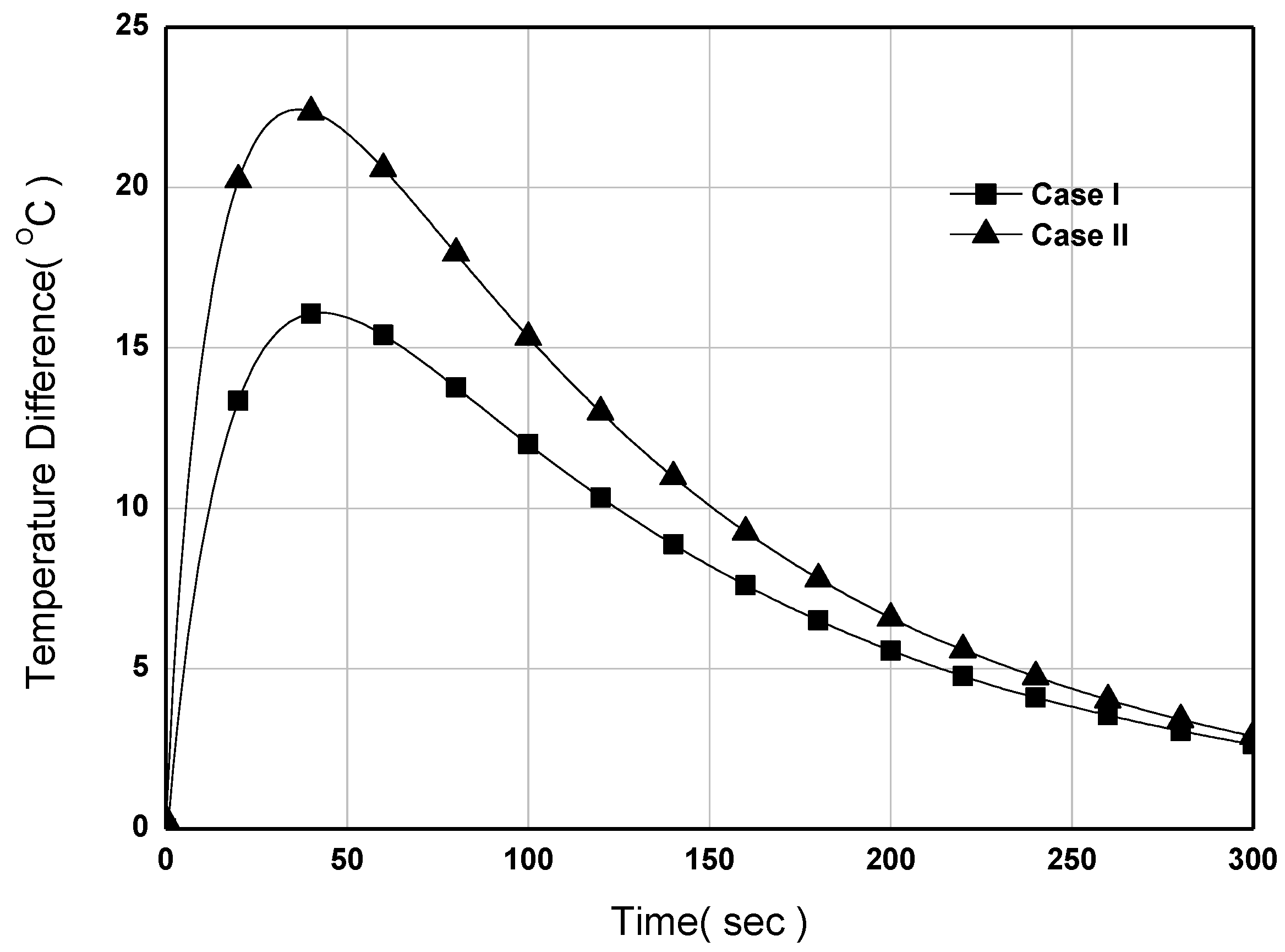
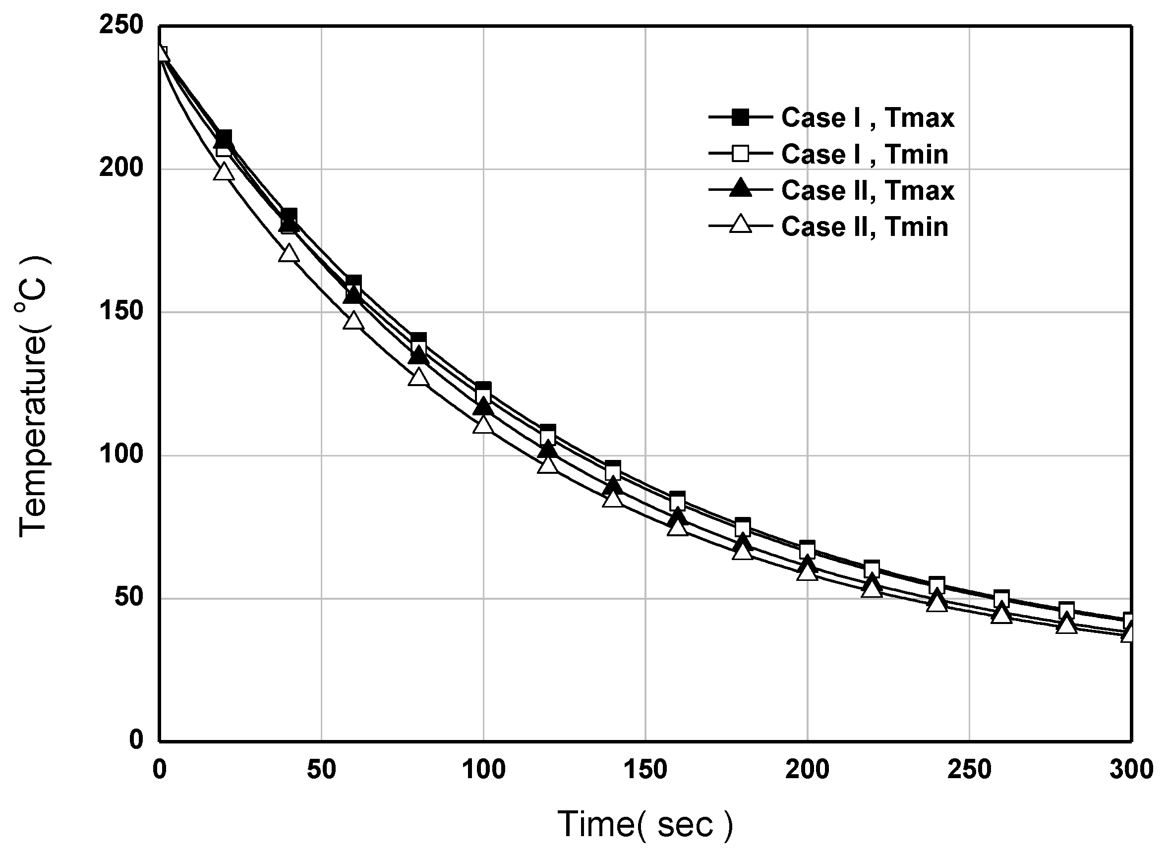
4. Results and Investigations
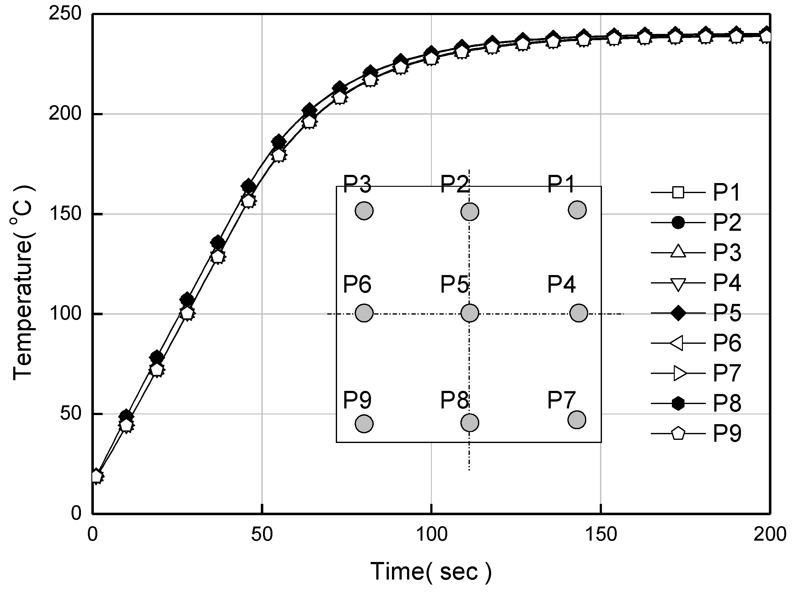
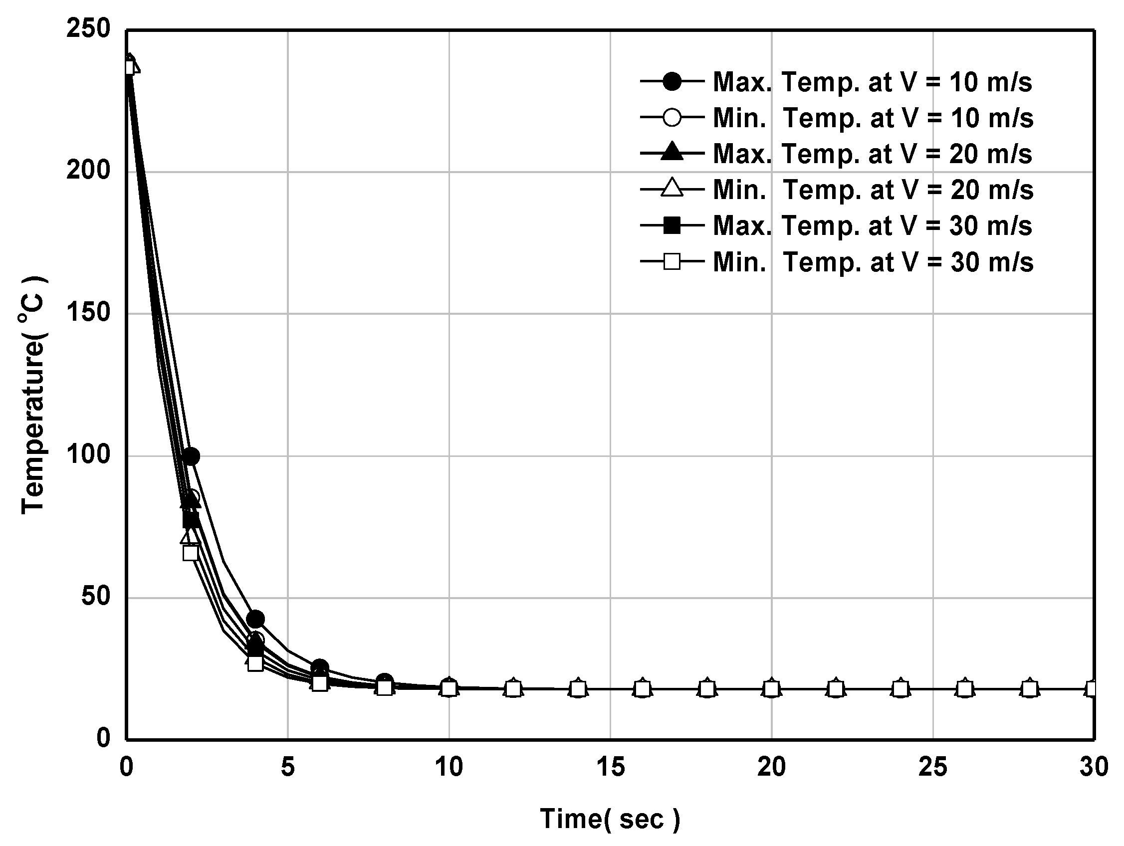
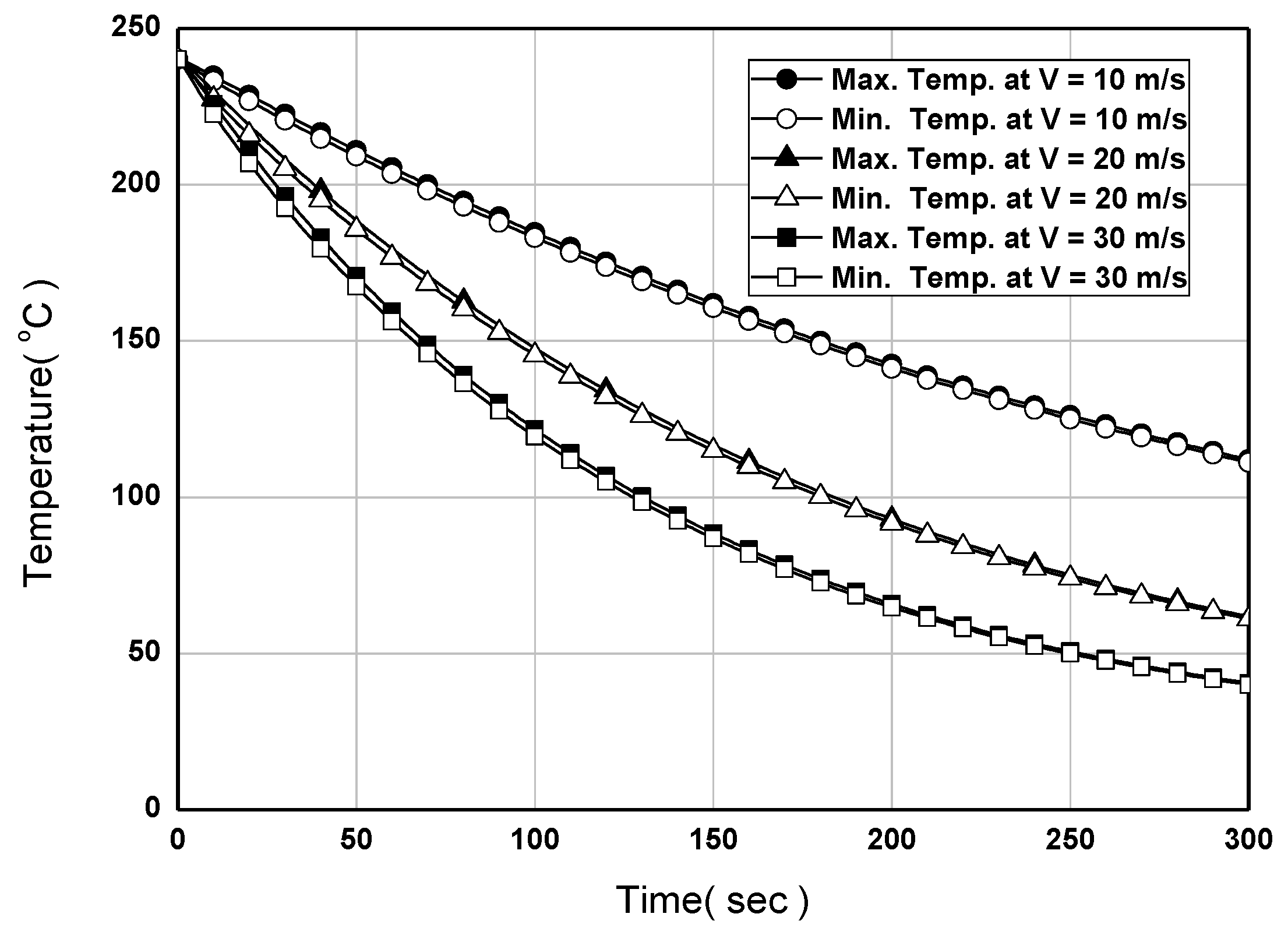
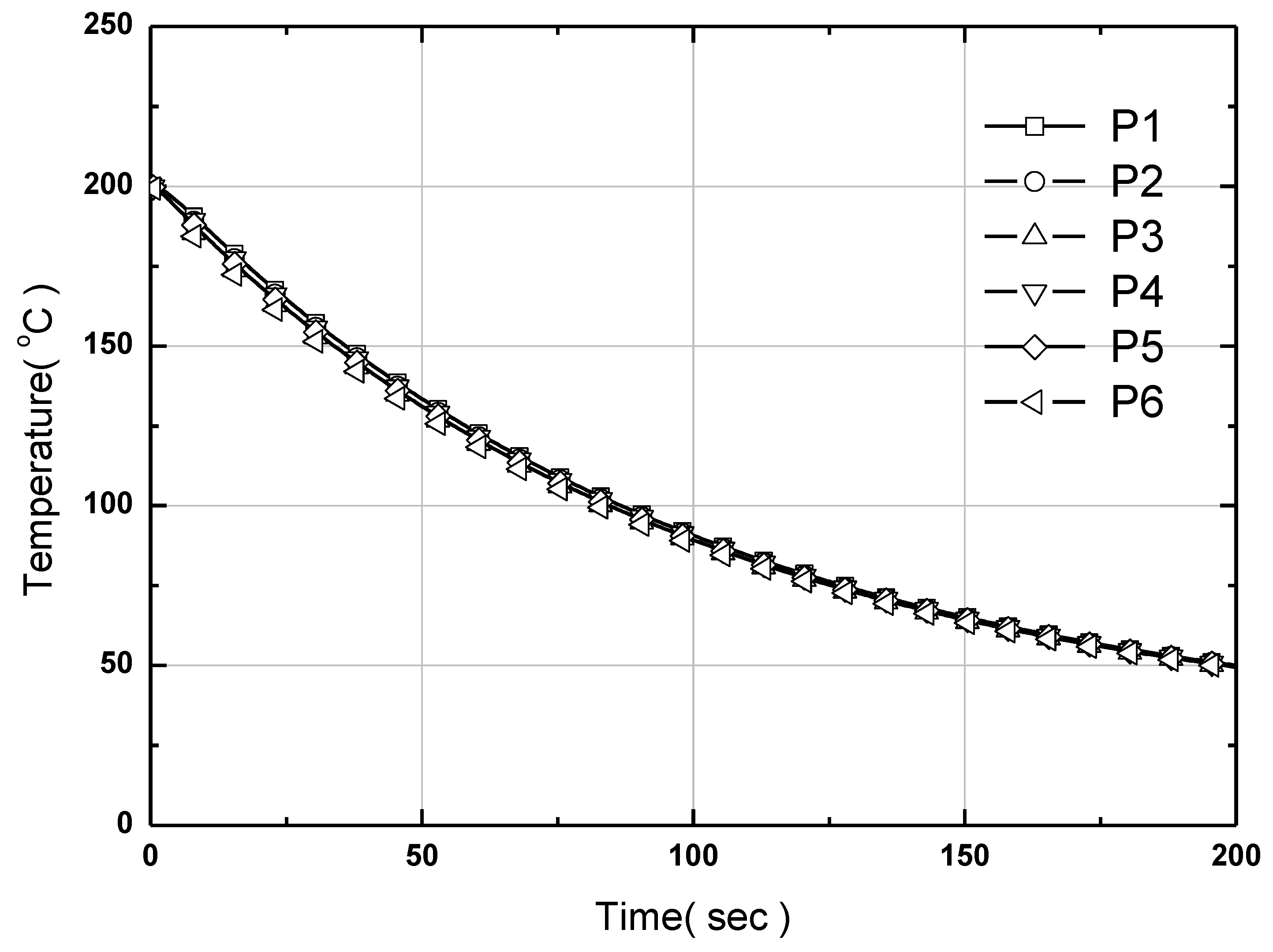
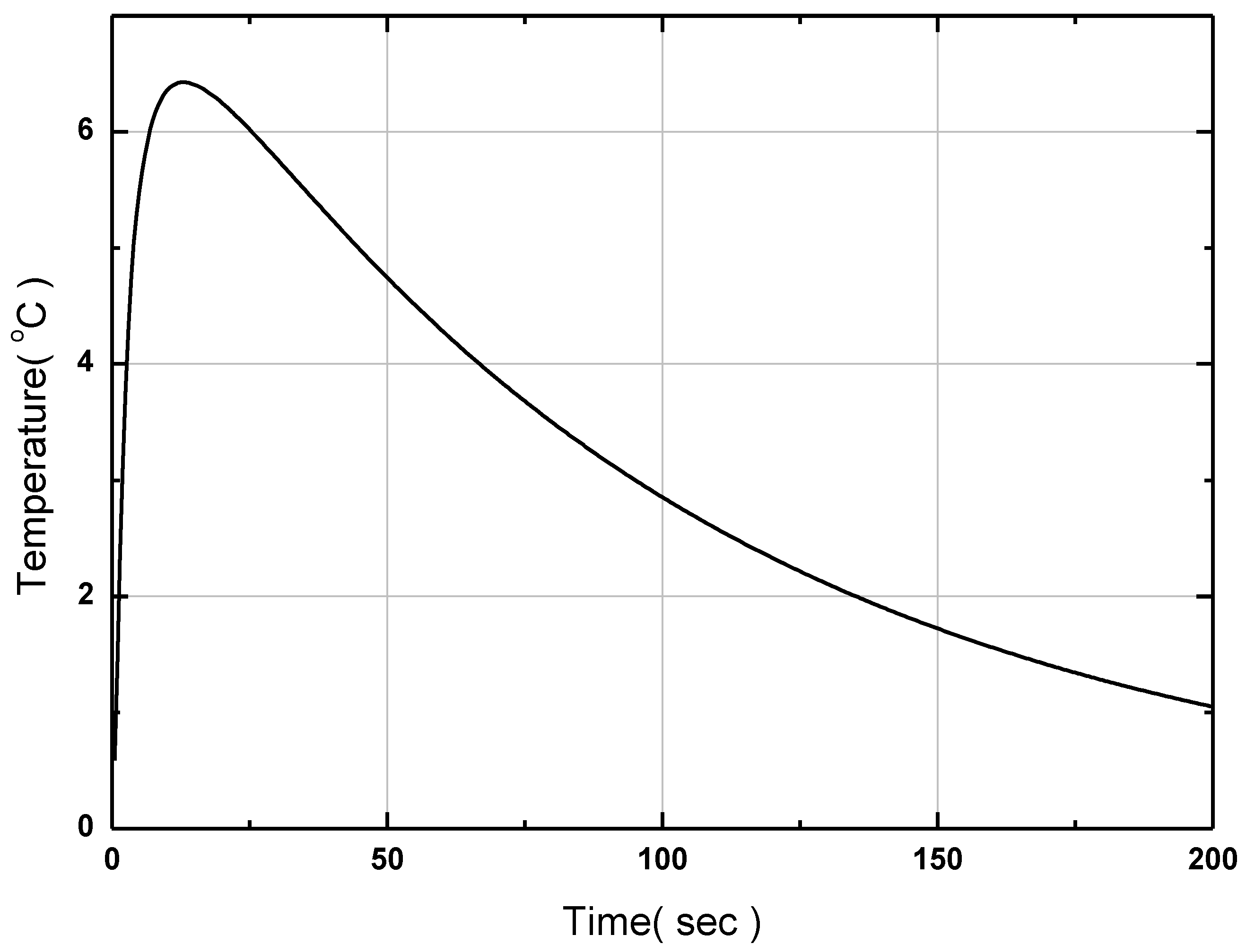
4.1. Heating Analysis Characteristics
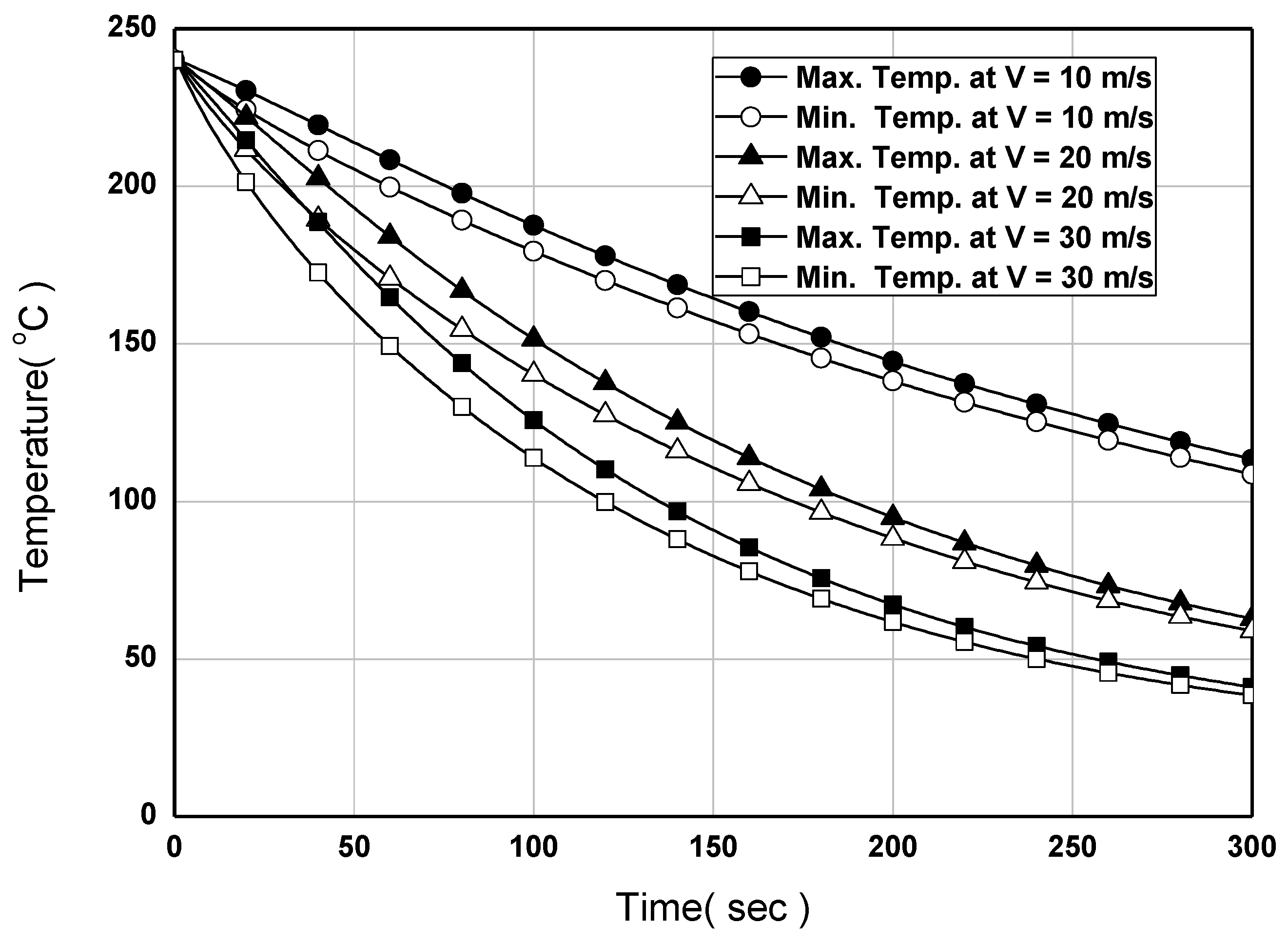
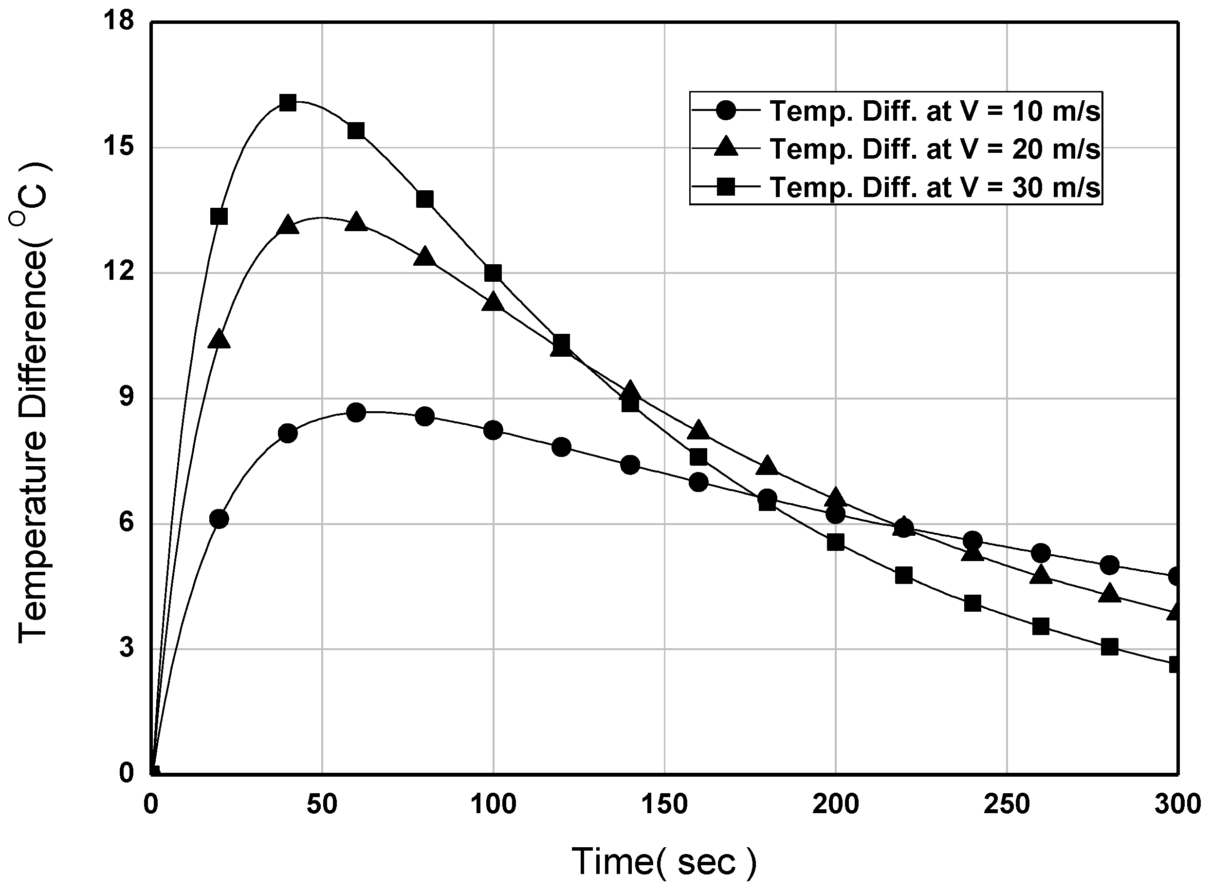
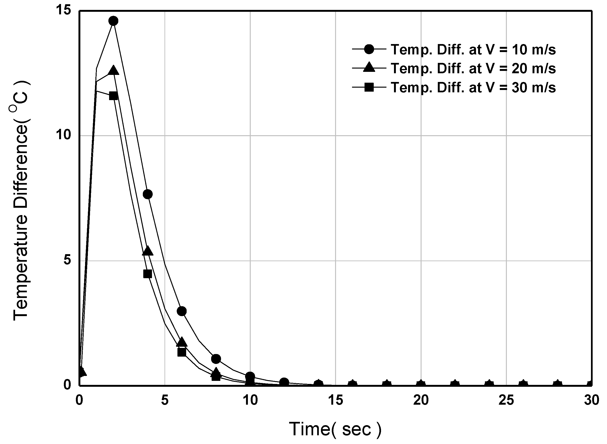
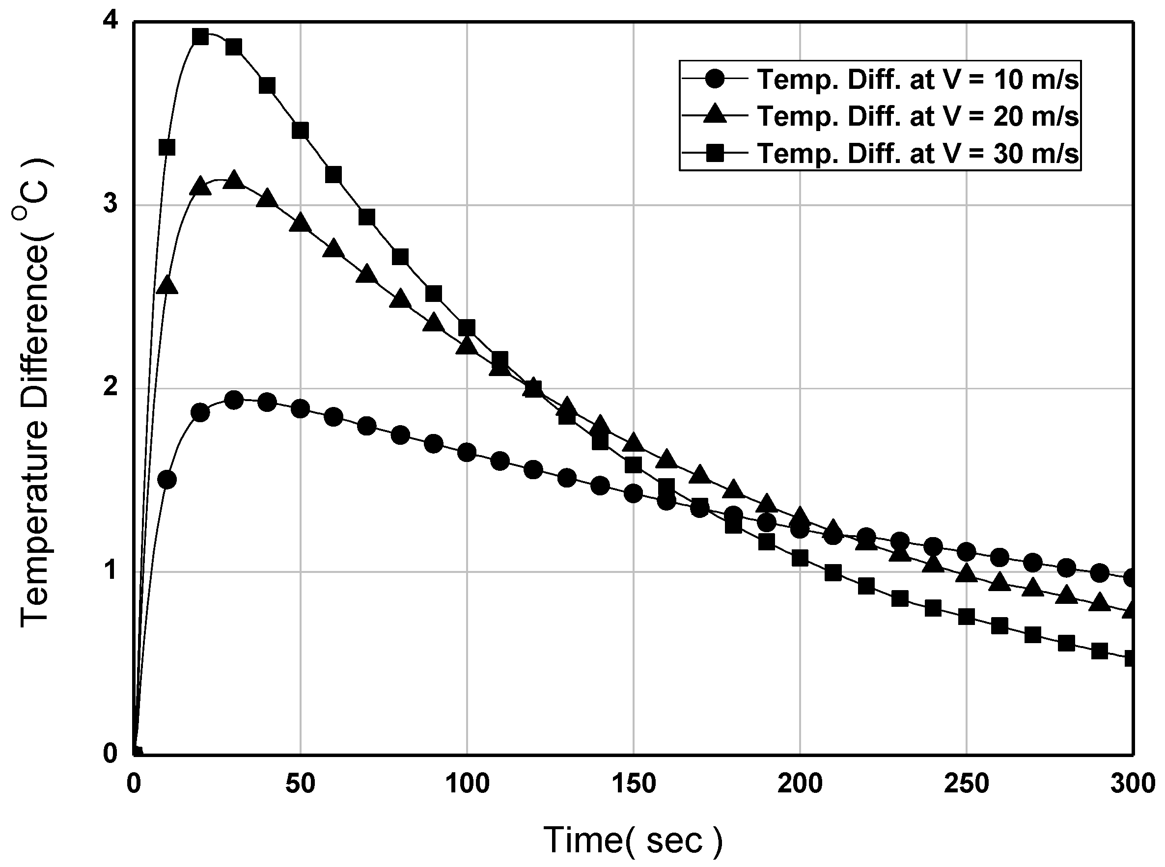
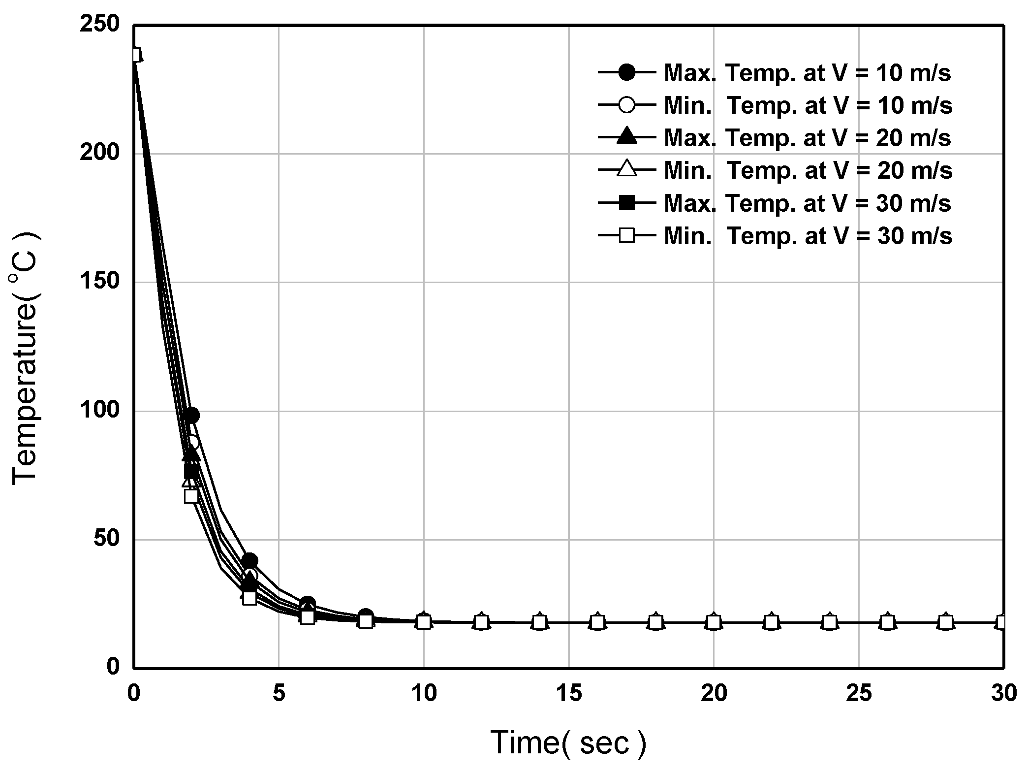
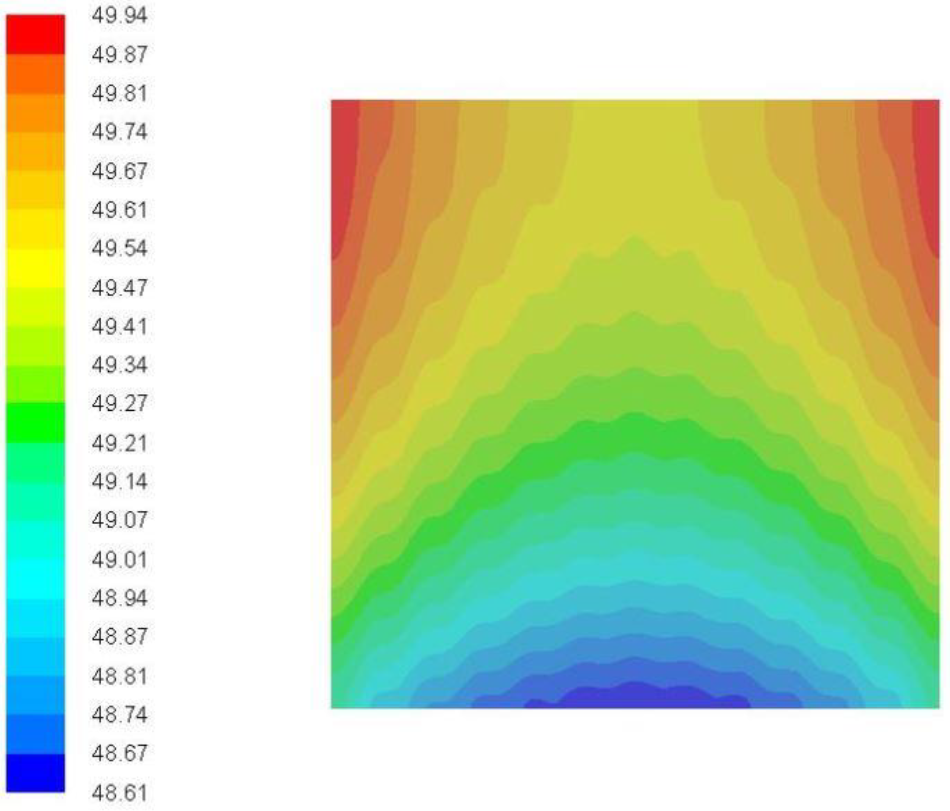
4.2. Cooling Analysis Characteristics
5. Conclusions
Author Contributions
Funding
Conflicts of Interest
References
- May, G.S.; Sze, S.M. Fundamentals of Semiconductor Fabrication; John Wily & Sons: New York, NY, USA, 2003. [Google Scholar]
- Chou, S.Y.; Krauss, P.R.; Renstrom, P.J. Nanoimprint Lithography. J. Vac. Sci. Technol. 1996, 14, 4129–4133. [Google Scholar] [CrossRef]
- Lee, J.; Park, S.; Choi, K.; Kim, G. Nano-scale patterning using the roll typed UVnanoimprint lithography tool. Microelectron. Eng. 2008, 85, 861–865. [Google Scholar] [CrossRef]
- Ahn, S.H.; Guo, L.J. Large-area roll-to-roll and roll-to-plate Nanoimprint Lithography: A step toward high-throughput application of continuous nanoimprinting. ACS Nano 2009, 3, 2304–2310. [Google Scholar] [CrossRef] [PubMed]
- Yoshikawa, H.; Taniguchi, J.; Tazaki, G.; Zento, T. Fabrication of high-aspect-ratio pattern via high throughput roll-to-roll ultraviolet nanoimprint lithography. Microelectron. Eng. 2013, 112, 273–277. [Google Scholar] [CrossRef]
- Hua, F.; Sun, Y.; Gaur, A.; Meitl, M.A.; Bilhaut, L.; Rotkina, L.; Wang, J.; Geil, P.; Shim, M.; Rogers, J.A.; et al. Polymer imprint lithography with molecular-scale resolution. Nano Lett. 2004, 4, 2467–2471. [Google Scholar] [CrossRef]
- Belligundu, S.; Shiakolas, P.S. Study on two-stage hot embossing microreplication: Silicon to polymer to polymer. J. Microlithogr. Microfabr. Microsyst. 2006, 5, 021103. [Google Scholar] [CrossRef]
- Jaszewski, R.W.; Schift, H.; Schnyder, B.; Schneuwly, A.; Gröning, P. Deposition of anti-adhesive ultra-thin teflon-like films and their interaction with polymers during hot embossing. Appl. Surface Sci. 1999, 143, 301–308. [Google Scholar] [CrossRef]
- Chou, S.Y.; Krauss, P.R.; Renstrom, P.J. Imprint of sub-25 nm vias and trenches in polymers. Appl. Phys. Lett. 1995, 67, 3114. [Google Scholar] [CrossRef]
- Youn, S.W.; Ogiwara, M.; Goto, H.; Takahashi, M.; Maeda, R. Prototype development of a roller imprint system and its application to large area polymer replication for a microstructured optical device. J. Mater. Process. Technol. 2008, 202, 76–85. [Google Scholar] [CrossRef]
- Xia, Q.; Keimel, C.; Ge, H.; Yu, Z.; Wu, W.; Chou, S.Y. Ultrafast patterning of nanostructures in polymers using laser assisted nanoimprint lithography. Appl. Phys. Lett. 2003, 83, 4417–4419. [Google Scholar] [CrossRef] [Green Version]
- Hsu, Q.C.; Lin, Y.T.; Chou, D.C.; Wu, C.D. Study on Nanoimprint Formability Considering the Anti-adhesion Layer for (CH2)n Polymer by Molecular Dynamics Simulation. Curr. Nanosci. 2012, 8, 424–431. [Google Scholar] [CrossRef]
- Maury, P.; Escalante, M.; Reinhoudt, D.N.; Huskens, J. Directed Assembly of Nanoparticles onto Polymer-Imprinted or Chemically Patterned Templates Fabricated by Nanoimprint Lithography. Adv. Mater. 2005, 17, 2718–2723. [Google Scholar] [CrossRef]
- Retolaza, A.; Juarros, A.; Ramiro, J.; Merino, S. Thermal roll to roll nanoimprint lithography for micropillars fabrication on thermoplastics. Microelectron. Eng. 2018, 193, 54–61. [Google Scholar] [CrossRef]
- Mohamed, K. Nanoimprint Lithography for Nanomanufacturing. In Comprehensive Nanoscience and Nanotechnology, 2nd ed.; Andrews, D., Lipson, R., Nann, T., Eds.; Academic Press: Cambridge, MA, USA, 2019; pp. 357–386. [Google Scholar]
- Becker, H.; Heim, U. Hot embossing as a method for the fabrication of polymer high aspect ratio structures. Sens. Actuators A Phys. 2000, 83, 130–135. [Google Scholar] [CrossRef]
- Tan, H.; Gilbertson, A.; Chou, S.Y. Roller nanoimprint lithography. J. Vac. Sci. Technol. B Microelectron. Nanometer Struct. 1998, 16, 3926. [Google Scholar] [CrossRef]
- Cui, B.; Keimel, C.; Chou, S.Y. Ultrafast direct imprinting of nanostructures in metals by pulsed laser melting. Nanotechnology 2010, 21, 045303. [Google Scholar] [CrossRef]
- Moore, S.; Gomez, J.; Lek, D.; You, B.H.; Kim, N.; Song, I.H. Experimental study of polymer microlens fabrication using partial-filling hot embossing technique. Microelectron. Eng. 2016, 162, 57–62. [Google Scholar] [CrossRef]
- Youn, S.W.; Goto, H.; Takahashi, M.; Oyama, S.; Mastutani, K.; Maeda, R. Fabrication of a micro patterned parylene-C master by hot-embossing and its application to metallic mold replication. J. Micromech. Microeng. 2007, 17, 1402. [Google Scholar] [CrossRef]
- Ahn, S.; Cha, J.; Myung, H.; Kim, S.M.; Kang, S. Continuous ultraviolet roll nanoimprinting process for replicating large-scale nano-and micropatterns. Appl. Phys. Lett. 2006, 89, 12–15. [Google Scholar] [CrossRef]
- Moro, M.; Taniguchi, J.; Hiwasa, S. Fabrication of antireflection structure film by roll-to-roll ultraviolet nanoimprint lithography. J. Vac. Sci. Technol. B Nanotechnol. Microelectron. Mater. Process. Meas. Phenom. 2014, 32, 06FG09. [Google Scholar] [CrossRef]
- Chou, S.Y.; Keimel, C.; Gu, J. Ultrafast and direct imprint of nanostructures in silicon. Nature 2002, 417, 835–837. [Google Scholar] [CrossRef] [PubMed]
- Pang, S.W. Direct nano-printing on Al substrate using a SiC mold. J. Vac. Sci. Technol. B Microelectron. Nanometer Struct. 1998, 16, 1145. [Google Scholar] [CrossRef]
- Hirai, Y.; Fujiwara, M.; Okuno, T.; Tanaka, Y.; Endo, M.; Irie, S.; Nakagawa, K.; Sasago, M. Study of the Resist Deformation in Nanoimprint Lithography. J. Vac. Sci. Technol. 2001, 19, 2811–2815. [Google Scholar] [CrossRef]
- MacIntyre, D.; Thoms, S. A study of resist flow during nanoimprint lithography. Microelectron. Eng. 2005, 78–79, 670–675. [Google Scholar] [CrossRef]
- Toralla, K.P.; De Girolamo, J.; Truffier-Boutry, D.; Gourgon, C.; Zelsmann, M. High flowability monomer resists for thermal nanoimprint lithography. Microelectron. Eng. 2009, 86, 779–782. [Google Scholar] [CrossRef]
- Beck, M.; Graczyk, M.; Maximov, I.; Sarwe, E.L.; Ling, T.G.I.; Keil, M.; Motelius, L. Improving Stamps or 10 nm Level Wafer Scale Nanoimprint Lithography. Microelectron. Eng. 2002, 61–62, 441–448. [Google Scholar] [CrossRef]
- Tormen, M.; Malureanu, R.; Pedersen, R.H.; Lorenzen, L.; Rasmussen, K.H.; Lüscher, C.J.; Kristensen, A.; Hansen, O. Fast thermal nanoimprint lithography by a stamp with integrated heater. Microelectron. Eng. 2008, 85, 1229–1232. [Google Scholar] [CrossRef]
- Khang, D.Y.; Kang, H.; Kim, T.; Lee, H.H. Low-Pressure Nanoimprint Lithography. Nano Lett. 2004, 633–637. [Google Scholar] [CrossRef]
- Lebib, A.; Chen, Y.; Cambril, E.; Youinou, P.; Studer, V.; Natali, M.; Pepin, A.; Janssen, H.; Sijbesma, R. Room-temperature and low-pressure nanoimprint lithography. Microelectron. Eng. 2002, 61, 371–377. [Google Scholar] [CrossRef]
- Kwak, H.S.; Park, G.J.; Son, B.C.; Lee, J.J.; Park, H.C. Design of a Hot plate with Rapid Cooling Capability or Thermal Nanoimprint Lithography. In Proceedings of the 2006 SICE-ICASE International Joint Conference, Busan, Korea, 18–21 October 2006; pp. 4897–4901. [Google Scholar]
- Park, G.J.; Kwak, H.S.; Shin, D.W.; Lee, J.J. Numerical Simulation of Thermal Control of a Hot Plate for Thermal Nanoimprint Lithography Machines. In Proceedings of the 3rd International Conference on Heating Cooling Technology, Seoul, Korea, 4 March 2007; pp. 321–327. [Google Scholar]
- Con, C.; Zhang, J.; Jahed, Z.; Tsui, T.Y.; Yavuz, M.; Cui, B. Thermal nanoimprint lithography using fluoropolymer mold. Microelectron. Eng. 2012, 98, 246–249. [Google Scholar] [CrossRef]
- Yakhot, V.; Orszag, S.A.; Thangam, S.; Gatski, T.B.; Speziale, C.G. Development of turbulence models for shear flows by a double expansion technique. Phys. Fluids A Fluid Dyn. 1992, 4, 1510–1520. [Google Scholar] [CrossRef] [Green Version]
- Yang, J.H. An Experimental Study on the Thermal Performance of a Hot Plate for Thermal Nanoimprint Lithography. Ph.D. Thesis, Kumoh National Institute of Technology, Gyeongsangbuk-do, Korea, 2008. [Google Scholar]
- Faghri, A. Heatpipe Science and Technology; Taylor & Francis: Abingdon, UK, 1995. [Google Scholar]
- Wallin, P. Heat Pipe: Selection of Working Fluid; Heat and Mass Trasfer Project Report; MVK160: Lund, Sweden, 2012; pp. 1–7. [Google Scholar]
- Cengel, Y.A. Heat and Mass Transfer; McGraw-Hill: New York, NY, USA, 2012; pp. 521–527. [Google Scholar]


| NIL Method | Process Details | Mold/Substrate | Resist Materials |
|---|---|---|---|
| Thermal NIL [20,21] | Thermal annealing of polymers at temperatures up to 50 °C above the glass transition temperature. | High hardness molds (Young’s modulus should be higher than that of resist): silicon, glasses, quartz, nickel, ceramics, Al oxideNote: thermal expansion coefficient of mold and substrate should match | Only thermoplastic polymers: polystyrene (PS), poly(methyl-methacrylate) (PMMA), polycarbonate (PC), polyethylene terephthalate (PET), siloxane copolymers (PDMS-b-PS, PDMS-g-PMMA), specified spin-on polymers |
| UV NIL at room temperature [3,4,5,22,23] | UV, EUV exposure | UV-transparent materials: quartz glass; soft stamps are more common for UV NIL: polydimethylsiloxane (PDMS), polyvinyl chloride (PVC), PMMA | Low viscosity UV-sensitive materials, ideally with low volume shrinkage after polymerization—usually liquid functionalized monomers or oligomers, CARs |
| UV NIL + thermal annealing [18,19] | Simultaneous UV exposure and substrate heating | UV-transparent materials | UV-curable polymers with better surface coverage and lower imprint temperatures as for T-NIL can be used |
© 2019 by the authors. Licensee MDPI, Basel, Switzerland. This article is an open access article distributed under the terms and conditions of the Creative Commons Attribution (CC BY) license (http://creativecommons.org/licenses/by/4.0/).
Share and Cite
Park, G.; Lee, C. Numerical Study on Thermal Design of a Large-Area Hot Plate with Heating and Cooling Capability for Thermal Nanoimprint Lithography. Appl. Sci. 2019, 9, 3100. https://doi.org/10.3390/app9153100
Park G, Lee C. Numerical Study on Thermal Design of a Large-Area Hot Plate with Heating and Cooling Capability for Thermal Nanoimprint Lithography. Applied Sciences. 2019; 9(15):3100. https://doi.org/10.3390/app9153100
Chicago/Turabian StylePark, Gyujin, and Changhee Lee. 2019. "Numerical Study on Thermal Design of a Large-Area Hot Plate with Heating and Cooling Capability for Thermal Nanoimprint Lithography" Applied Sciences 9, no. 15: 3100. https://doi.org/10.3390/app9153100