Performance Analysis and Parameter Optimization of the Optimal Fixed-Point Quantum Search

Abstract

The optimal fixed-point quantum search (OFPQS) algorithm [Phys. Rev. Lett. 113, 210501 (2014)] achieves both the fixed-point property and quadratic speedup over classical algorithms, which gives a sufficient condition on the number of iterations to ensure the success probability is no less than a given lower bound (denoted by $1-{\delta }^2$). However, this condition is approximate and not exact. In this paper, we derive the sufficient and necessary condition on the number of feasible iterations, based on which the exact least number of iterations can be obtained. For example, when $\delta =0.8$, iterations can be saved by almost 25%. Moreover, to find a target item certainly, setting directly $1-{\delta }^2=100\%$, the quadratic advantage of the OFPQS algorithm will be lost, then, applying the OFPQS algorithm with $1-{\delta }^2<100\%$ requires multiple executions, which leads to a natural problem of choosing the optimal parameter $\delta$. For this, we analyze the extreme and minimum properties of the success probability and further analytically derive the optimal $\delta$ which minimizes the query complexity. Our study can be a guideline for both the theoretical and application research on the fixed-point quantum search algorithms.

1. Introduction

Grover search [1,2] provides a quadratic speedup over classical search algorithms, and has been proven optimal [3,4,5,6]. However, there still exists the soufflé problem [7], i.e., the success probability will decline if the algorithm iterates too many times. Therefore, the Grover algorithm can only apply to the case where the optimal number of iterations [8] can be determined.

Based on the quantum amplitude amplification [9,10,11,12] and phase-matching methods [13,14,15,16], a fixed-point quantum search algorithm [17] has been proposed, where the final state of the algorithm converges to the target states and the success probability increases as the number of iterations grows. This algorithm applies to the case where the lower bound (denoted by ${\lambda }_0$) of the fraction of target items (denoted by $\lambda$) is known. However, the advantage of quadratic speedup is lost [18,19].

Fortunately, Yoder et al. developed the optimal fixed-point quantum search (OFPQS) algorithm [20], which achieves both the fixed-point property and optimal query complexity, where the success probability for any unknown $\lambda \ge {\lambda }_0$ can be always no less than a given value (denoted by $1-{\delta }^2$) between 0 and 1, as long as the given condition on the number of iterations is satisfied. However, this condition is approximate and not tight, i.e., the required number of iterations might be further reduced.

In addition, the lower bound of success probability $1-{\delta }^2$ of the OFPQS algorithm is lower than 100%, because setting $\delta =0$, the algorithm will change back to the original fixed-point algorithm [17] and thus lose the quadratic speedup [20]. However, in practical search problems, it is often desired to find a target item eventually, rather than just succeed with probability above a lower bound. For this, a natural strategy is to make multiple trials of the OFPQS algorithm with $\delta >0$ until success. This brings up a new problem, that is, how to choose the optimal parameters to find a target item as soon as possible.

In this paper, we expect to give the minimum feasible number of iterations, analyze the extreme and minimum properties of the success probability, and further derive the optimal parameter of the OFPQS algorithm to find a target item with the minimum query complexity.

The paper is organized as follows: In Section 2, we briefly introduce the OFPQS algorithm. In Section 3, we derive the optimal number of iterations and analyze the properties of the success probability of OFPQS algorithm. In Section 4, we give the selection method of optimal parameter $\delta$. Section 5 comprises of discussions about the effects of the optimal number of iterations and the optimal $\delta$, as well as the upper bound of expected queries of applying the OFPQS algorithm to find a target item certainly. Finally, a brief conclusion is given in Section 6.

2. OFPQS Algorithm Revisited

Based on the multi-phase matching method [21,22], the OFPQS algorithm [20] overcomes the souffle problem in the original Grover algorithm [1] as well as the loss of quadratic speedup in the original fixed-point quantum search algorithm [17].

The initial state of the OFPQS algorithm is prepared to be $\left|\psi \right.⟩=A\left|0\right.⟩$, where A can be an arbitrary unitary operator. Denote the equal superposition of all target and nontarget states as $\left|\alpha \right.⟩$ and $\left|\beta \right.⟩$, respectively, i.e.,

$$\begin{array}{ccc}\hfill \left|\alpha \right.⟩& =& \frac{1}{\sqrt{M}}\sum _{x\in f^{-1}\left(1\right)}\left|x\right.⟩,\hfill \end{array}$$

(1)

$$\begin{array}{ccc}\hfill \left|\beta \right.⟩& =& \frac{1}{\sqrt{N-M}}\sum _{x\in f^{-1}\left(0\right)}\left|x\right.⟩,\hfill \end{array}$$

(2)

where M is the number of target items in the database of size N, $f\left(x\right)$ is a Boolean function identifying the target state(s), i.e., if $\left|x\right.⟩$ is a target state, then $f\left(x\right)=1$—otherwise, $f\left(x\right)=0$, with $A=H^{\otimes n}$ and H being the Hadamard transform, $\left|\psi \right.⟩$ can be written as

$$\begin{array}{ccc}\hfill \left|\psi \right.⟩& =& \sqrt{\lambda }\left|\alpha \right.⟩+\sqrt{1-\lambda }\left|\beta \right.⟩,\hfill \end{array}$$

(3)

where $\lambda =M/N$ represents the fraction of target items.

The sequence of operations performed on $\left|\psi \right.⟩$ is given by (see also Equation (2.6) of [21])

$$S_L=G\left({\varphi }_l,{\phi }_l\right)G\left({\varphi }_{l-1},{\phi }_{l-1}\right)\cdots G\left({\varphi }_1,{\phi }_1\right),$$

(4)

where $L-1=2l$ represents the query complexity of sequence $S_L$, as each generalized Grover operation $G\left({\varphi }_j,{\phi }_j\right)$ requires two Oracle queries [20], and

$$\begin{array}{ccc}\hfill G\left({\varphi }_j,{\phi }_j\right)& =& -A{S}_0^{{\varphi }_j}{A}^{†}{S}_f^{{\phi }_j},\hfill \end{array}$$

(5)

where $S_0^{{\varphi }_j}$ and $S_f^{{\phi }_j}$ are the selective phase shifts ($i=\sqrt{-1}$) (see also Equations (1) and (2) of [13]),

$$\begin{array}{ccc}\hfill S_0^{{\varphi }_j}& =& I-\left(1-e^{i{\varphi }_j}\right)\left|0\right.⟩\left.⟨0\right|,\hfill \end{array}$$

(6)

$$\begin{array}{ccc}\hfill S_f^{{\phi }_j}& =& I-\left(1-e^{i{\phi }_j}\right)\sum _{x\in f^{-1}\left(1\right)}\left|x\right.⟩\left.⟨x\right|.\hfill \end{array}$$

(7)

Under the multiphase matching condition (see also Equation (11) of [20])

$${\varphi }_j={\phi }_{l-j+1}=-2{cot}^{-1}\left(tan\left(2\pi j/L\right)\sqrt{1-{\gamma }^2}\right),1\le j\le l,$$

(8)

the final state can be obtained as

$$S_L\left|\psi \right.⟩=\sqrt{P_L}\left|\alpha \right.⟩+\sqrt{1-P_L}\left|\beta \right.⟩,$$

(9)

where $\gamma =T_{1/L}^{-1}\left(1/\delta \right)$, $P_L$ is the success probability of the algorithm (see also Equation (1) of [20]),

$$P_L=1-{\delta }^2{T}_L^2\left[T_{1/L}\left(1/\delta \right)\sqrt{1-\lambda }\right],$$

(10)

and $T_L\left(x\right)$ is the Lth Chebyshev polynomial of the first kind [23],

$$T_L\left(x\right)=\left\{\begin{array}{ll}cos\left(Larccos\left(x\right)\right),\hfill & \mathrm{if}\left|x\right|\le 1,\\ cosh\left(L\mathrm{arcosh}\left(x\right)\right),\hfill & \mathrm{if}x\ge 1,\\ {\left(-1\right)}^{L}cosh\left(L\mathrm{arcosh}\left(-x\right)\right),\hfill & \mathrm{if}x\le -1.\end{array}\right.$$

(11)

To ensure the success probability $P_L\left(\lambda \right)$ no less than a given lower bound $1-{\delta }^2$ for any $\delta \in \left(0,1\right]$, an approximated condition of L is given as

$$L\ge \frac{ln\left(2/\delta \right)}{\sqrt{\lambda }},$$

(12)

which is sufficient but not necessary, as shown below.

3. Performance Analysis of the OFPQS Algorithm

After deep theoretical analysis, we can obtain three new properties on the number of iterations and success probability of the OFPQS algorithm, which are as follows.

Property 1.

Given a lower bound ${\lambda }_0$ of the fraction λ of target items, the least exact number of iterations l (denoted by $l_{opt}$) of the OFPQS algorithm that enables the success probability $P_L\left(\lambda \right)\ge 1-{\delta }^2$ for any $\lambda \ge {\lambda }_0$ with $L=2l+1$, can be given in the form

$$l_{opt}=⌈\frac{\mathrm{arcosh}\left(1/\delta \right)}{2\mathrm{arcosh}\left(1/\sqrt{1-{\lambda }_0}\right)}-\frac{1}{2}⌉.$$

(13)

Proof. 

Based on Equation (10), for arbitrary $\lambda \in \left(0,1\right)$ and $\delta \in \left(0,1\right]$, a necessary and sufficient condition to make the success probability $P_L\left(\lambda \right)\ge 1-{\delta }^2$ can be given as follows,

$$\left|T_{1/L}\left(1/\delta \right)\right|\sqrt{1-\lambda }\le 1,$$

(14)

due to the fact that

$$\left|T_L\left(x\right)\right|\le 1\iff \left|x\right|\le 1.$$

(15)

Note that if $\left|x\right|>1$, then, $\mathrm{arcosh}\left(\left|x\right|\right)>0$ and $\left|T_L\left(x\right)\right|=cosh\left(L\mathrm{arcosh}\left(\left|x\right|\right)\right)>1$; if $\left|x\right|\le 1$, then, $\left|T_L\left(x\right)\right|=\left|cos\left(Larccos\left(x\right)\right)\right|\le 1$. Due to $T_{1/L}\left(1/\delta \right)\ge 1$ and $cosh\left(x\right)$ monotonically increases for $x\ge 0$, Equation (14) can be further reduced to

$$\begin{array}{ccc}\hfill L& \ge & \frac{\mathrm{arcosh}\left(1/\delta \right)}{\mathrm{arcosh}\left(1/\sqrt{1-\lambda }\right)}.\hfill \end{array}$$

(16)

Then, according to $L=2l+1$, we have

$$l\ge ⌈\frac{\mathrm{arcosh}\left(1/\delta \right)}{2\mathrm{arcosh}\left(1/\sqrt{1-\lambda }\right)}-\frac{1}{2}⌉.$$

(17)

Therefore, to ensure that $P_L\left(\lambda \right)\ge 1-{\delta }^2$ for any $\lambda \ge {\lambda }_0$, the least number of iterations, expressed by Equation (13), can be finally obtained. □

Property 2.

The extreme properties of the success probability $P_L\left(\lambda \right)$ as a function of $\lambda \in \left(0,1\right)$ can be given as follows (see Proof in Appendix A):

For $\delta \in \left(0,1\right]$, when $L>1$, $P_L\left(\lambda \right)$ has $\left(L-1\right)/2\equiv l$ local maximum points

$${\lambda }_{max,j}=1-{\gamma }^2{cos}^2\left(\frac{2j-1}{2L}\pi \right),j=1,2,\cdots ,l,$$

(18)

and l local minimum points

$${\lambda }_{min,j}=1-{\gamma }^2{cos}^2\left(\frac{j}{L}\pi \right),j=1,2,\cdots ,l.$$

(19)

When $L=1$, there are no local extreme points.

Property 3.

The success probability $P_L\left(\lambda \right)$ with $L=2l_{opt}+1\equiv L_{opt}$ has a minimum value (denoted by $P_{min}$) on the range $\lambda \in \left[{\lambda }_0,1\right)$ for ${\lambda }_0\le 4/5$, which can be written as (for a proof, see Appendix B)

$$\begin{array}{ccc}\hfill P_{min}& \equiv & min\left\{P_{L_{opt}}\left(\lambda \right):\lambda \ge {\lambda }_0\right\}\hfill \\ & =& \left\{\begin{array}{cc}1-{\delta }^2,\hfill & \mathrm{if}\delta <\sqrt{1-{\lambda }_0},\\ {\lambda }_0,\hfill & \mathrm{if}\delta \ge \sqrt{1-{\lambda }_0}.\end{array}\right.\hfill \end{array}$$

(20)

Note that the case ${\lambda }_0>4/5$ can already be well disposed of by classical search.

4. Optimization of Parameters of the OFPQS Algorithm

In practical applications of the OFPQS algorithm, if set $\delta =0$, then, from Equation (12) or Equation (13) it can be found that the quadratic speedup over classical algorithms will be lost; while, if set $\delta >0$, the output of the OFPQS algorithm is not necessarily a target item. Inspired by [4], which achieves about 12% reduction of the expected queries through stopping the Grover algorithm short of the optimal number of iterations and restarting again in case of failure, to find a target item as soon as possible, a natural strategy is to set the lower bound of success probability $1-{\delta }^2<100\%$ and repeat the OFPQS algorithm until it succeeds. Under this strategy, in order to find the optimal parameter $\delta$, we shall estimate the expected number of Oracle queries of the OFPQS algorithm before a target item is found.

First, a single execution of the OFPQS algorithm requires at least $2l_{opt}$ queries, since $l_{opt}$ iterations are required in the sequence $S_L$ of Equation (4). Second, judging whether the algorithm is successful from the measurement result also takes one query. Then, define $L_{opt}=2l_{opt}+1$, we can get the expected number of Oracle queries as

$$\begin{array}{ccc}\hfill L_E& =& \sum _{j=1}^{\infty }{p}_j{L}_{opt},\hfill \end{array}$$

(21)

where

$$p_j={\left[1-P_{L_{opt}}\left(\lambda \right)\right]}^{j-1}$$

(22)

is the probability of occurrence of the j-th execution of the OFPQS algorithm. From Equations (20)–(22), we can further obtain that

$$\begin{array}{ccc}\hfill L_E& \le & \sum _{j=1}^{\infty }{\left(1-P_{min}\right)}^{j-1}{L}_{opt}\hfill \\ & =& \left(2l_{opt}+1\right)/P_{min}\equiv L_E^{Up},\hfill \end{array}$$

(23)

where $L_E^{Up}$ represents the upper bound of $L_E$.

We can define the optimal $\delta$ as the one that makes the upper bound of expected number of queries $L_E^{Up}$ as few as possible. Detailed analysis shows that such optimal $\delta$ (denoted by ${\delta }_{opt}$) exists and can be analytically written in the following form (Proof see Appendix C),

$${\delta }_{opt}=\left\{\begin{array}{cc}{\delta }_k,\hfill & \mathrm{if}{\lambda }_0\in \left[\lambda {}_{0,k},\lambda {}_{0,k-1}\right],k\ge 1,\hfill \\ \forall \delta \in \left[{\delta }_0,1\right),\hfill & \mathrm{if}{\lambda }_0\in \left[\lambda {}_{0,0},4/5\right],\hfill \end{array}\right.$$

(24)

where

$${\delta }_k=T_{2k+1}^{-1}\left(1/\sqrt{1-{\lambda }_0}\right),$$

(25)

$T_L\left(x\right)$ is defined by Equation (11),

$$\lambda {}_{0,k-1}=1-{cosh}^{-2}\left(y_{k-1}\right),k\ge 1,$$

(26)

$y_{k-1}$ is the unique solution of equation

$$\begin{array}{c}\hfill {sinh}^2\left(4ky\right)+{sinh}^2\left(2y\right)-4ksinh\left(4ky\right)sinh\left(2y\right)=0,\frac{x}{4k+2}<y<\frac{x}{4k-2},\end{array}$$

(27)

and x satisfies

$$sinh\left(x\right)-2x=0,x>0.$$

(28)

Note that, when ${\lambda }_0={\lambda }_{0,k}$ ($k\ge 0$) or ${\lambda }_{0,0}\le {\lambda }_0\le 4/5$, the corresponding ${\delta }_{opt}$ has multiple values, as shown in Figure 1.

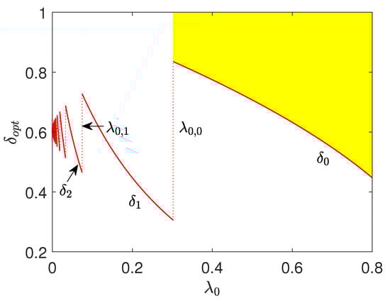
Figure 1. (Color online.) The optimal parameter ${\delta }_{opt}$ as a function of the lower bound ${\lambda }_0$ of the fraction of target items. The red solid curves, red dotted vertical lines and the yellow (gray) area represent ${\delta }_k$, $\lambda {}_{0,k}$ ($k\ge 0$), and the value of ${\delta }_{opt}$ for $\lambda {}_{0,0}\le {\lambda }_0\le 4/5$, respectively.

Note that, with the above optimal parameters, we can obtain the corresponding upper bound of the expected number of queries, i.e.,

$$L_{E,opt}^{Up}\left({\lambda }_0\right)\equiv L_E^{Up}\left({\lambda }_0,l_{opt},{\delta }_{opt}\right).$$

(29)

5. Discussion

In this section, the effects of optimal parameters $l_{opt}$ of Equation (13) and ${\delta }_{opt}$ of Equation (24), and the complexity of $L_{E,opt}^{Up}\left({\lambda }_0\right)$ of Equation (29) are discussed as follows.

5.1. Effects of $l_{opt}$ and ${\delta }_{opt}$

Different from our optimal number of iterations $l_{opt}$ of Equation (13), to achieve a success probability no less than $1-{\delta }^2$ for any $\lambda \ge {\lambda }_0$ in the OFPQS algorithm [20], another number of iterations can be obtained from Equation (12), denoted by

$$l_{min}^{{\mathrm{Yoder}}^{\prime }\mathrm{s}}\equiv ⌈\frac{ln\left(2/\delta \right)}{2\sqrt{{\lambda }_0}}-\frac{1}{2}⌉.$$

(30)

As a comparison, Figure 2 shows some examples of the success probability $P_L\left(\lambda \right)$ for the different number of iterations l with $L=2l+1$. We can see that both $l=l_{min}^{{\mathrm{Yoder}}^{\prime }\mathrm{s}}$ and $l=l_{opt}$ can achieve the goal $P_L\left(\lambda \right)\ge 1-{\delta }^2$ for $\lambda \ge {\lambda }_0$; while $l=l_{opt}-1$ can’t. Therefore, $l_{opt}$ is just the least number of iterations required. When ${\lambda }_0\ll 1$, $\mathrm{arcosh}\left(1/\sqrt{1-{\lambda }_0}\right)\approx \sqrt{{\lambda }_0}$, then, from Equations (13) and (30) it follows that

$$l_{opt}/l_{min}^{{\mathrm{Yoder}}^{\prime }\mathrm{s}}\approx \frac{\mathrm{arcosh}\left(1/\delta \right)}{ln\left(2/\delta \right)},$$

(31)

which is shown in the inset of Figure 2.

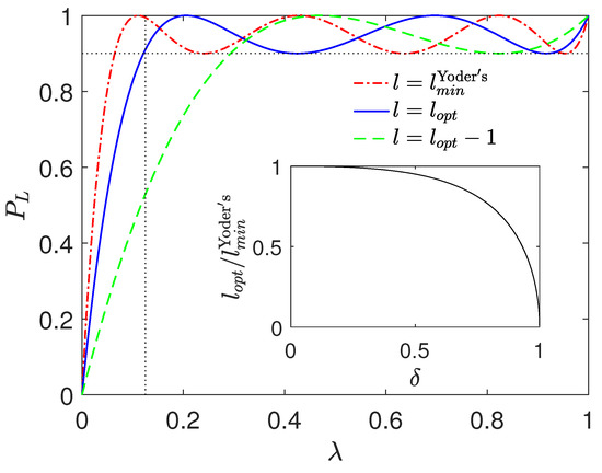
Figure 2. (Color online.) The success probability $P_L$ versus the fraction of target items $\lambda$ for different number of iterations l with $L=2l+1$, $\lambda \ge {\lambda }_0=0.125$ (dotted vertical line) and $P_L\ge 1-{\delta }^2=0.9$ (dotted horizontal line). The red dashed-dotted, blue solid, and green dashed curves correspond to $l=l_{min}^{{\mathrm{Yoder}}^{\prime }\mathrm{s}}=3$, $l=l_{opt}=2$ and $l=l_{opt}-1$, respectively. Inset: We plot $l_{opt}/l_{min}^{{\mathrm{Yoder}}^{\prime }\mathrm{s}}$ against $\delta$ with ${\lambda }_0\ll 1$.

We can see that when $\delta \to 1$, $l_{opt}/l_{min}^{{\mathrm{Yoder}}^{\prime }\mathrm{s}}\to 0$. For example, when $\delta =0.8$, $l_{opt}/l_{min}^{{\mathrm{Yoder}}^{\prime }\mathrm{s}}\approx 75.65\%$, almost a quarter of iterations can be saved.

For any given lower bound ${\lambda }_0\in \left(0,4/5\right]$ of the fraction of target items, by theoretical analysis we have obtained the analytical expression of the optimal $\delta$, i.e., ${\delta }_{opt}$ defined by Equation (24). In order to compare the results of $\delta ={\delta }_{opt}$ and $\delta \ne {\delta }_{opt}$ with $l=l_{opt}\left(\delta \right)$, we define $L_{E,rel}^{Up,nor}\left({\lambda }_0,\delta \right)$ to be the normalized relative value of $L_E^{Up}\left({\lambda }_0,\delta \right)$ with respect to $L_E^{Up}\left({\lambda }_0,{\delta }_{opt}\right)$, i.e.,

$$\begin{array}{ccc}\hfill L_{E,rel}^{Up,nor}\left({\lambda }_0,\delta \right)& =& \frac{L_{E,rel}^{Up}\left({\lambda }_0,\delta \right)}{max\left\{L_{E,rel}^{Up}\left({\lambda }_0,\delta \right):0<\delta \le 1\right\}},\hfill \end{array}$$

(32)

where

$$\begin{array}{c}\hfill L_{E,rel}^{Up}\left({\lambda }_0,\delta \right)=lnln\left(L_E^{Up}\left({\lambda }_0,\delta \right)\right)-lnln\left(L_E^{Up}\left({\lambda }_0,{\delta }_{opt}\right)\right).\end{array}$$

(33)

The dependence of $L_{E,rel}^{Up,nor}\left({\lambda }_0,\delta \right)$ on ${\lambda }_0$ and $\delta$ is shown in Figure 3, where the darker the color, the smaller the value. For ease of comparison, ${\delta }_{opt}$ is marked by the white dashed curves. We can see that the color in the area corresponding to ${\delta }_{opt}$ is darkest, which indicates that the optimal parameter ${\delta }_{opt}$ indeed enables the upper bound of expected queries to reach the minimum.

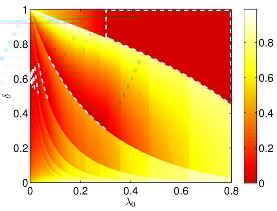
Figure 3. (Color online.) The normalized relative value $L_{E,rel}^{Up,nor}\left({\lambda }_0,\delta \right)$ as a function of $\delta$ and ${\lambda }_0$. The white dashed curves correspond to the optimal parameter ${\delta }_{opt}$ of Equation (24).

5.2. Complexity of $L_{E,opt}^{Up}\left({\lambda }_0\right)$

Based on Equations (13), (20), (23), (24), and (29), we can obtain the expression of $L_{E,opt}^{Up}\left({\lambda }_0\right)$ as below:

$$\begin{array}{ccc}\hfill L_{E,opt}^{Up}\left({\lambda }_0\right)& =& \left\{\begin{array}{ll}\frac{2k+1}{1-{\delta }_k^2},\hfill & \mathrm{if}{\lambda }_0\in \left[\lambda {}_{0,k},\lambda {}_{0,k-1}\right),k\ge 1,\\ \frac{1}{1-{\delta }_0^2},\hfill & \mathrm{if}{\lambda }_0\in \left[\lambda {}_{0,0},4/5\right],\end{array}\right.\hfill \end{array}$$

(34)

where ${\delta }_k$ and $\lambda {}_{0,k-1}$ are defined by Equations (25) and (26), respectively. To analyze the complexity of $L_{E,opt}^{Up}\left({\lambda }_0\right)$, first, for any known ${\lambda }_0\ll 1$, we can determine an integer

$$k=⌈\frac{x}{4\mathrm{arcosh}\left(1/\sqrt{1-{\lambda }_0}\right)}-\frac{1}{2}⌉,$$

(35)

such that ${\lambda }_0\in \left[{\lambda }_{0,k}^{\prime },{\lambda }_{0,k-1}^{\prime }\right)$, where ${\lambda }_{0,k}^{\prime }$ is as defined by Equation (A26) and $x>0$ is the solution of Equation (28). From Equations (26) and (27) it follows that

$${\lambda }_{0,k}^{\prime }\le {\lambda }_{0,k-1}<{\lambda }_{0,k-1}^{\prime },$$

(36)

then, we have ${\lambda }_0\in \left[\lambda {}_{0,k},\lambda {}_{0,k-2}\right)$. When ${\lambda }_0\ll 1$, $k\to \infty$, $k\approx k-1$, thus,

$$L_{E,opt}^{Up}\left({\lambda }_0\right)\approx \frac{2k+1}{1-{\delta }_k^2},$$

(37)

where

$${\delta }_k\approx {cosh}^{-1}\left(\frac{x}{2}\right)$$

(38)

due to $k\approx \frac{x}{4\mathrm{arcosh}\left(1/\sqrt{1-{\lambda }_0}\right)}-\frac{1}{2}$, and

$$k\approx \frac{x}{4\sqrt{{\lambda }_0}}-\frac{1}{2}$$

(39)

due to $\mathrm{arcosh}\left(1/\sqrt{1-{\lambda }_0}\right)\approx \sqrt{{\lambda }_0}$. Combining Equations (37), (38), and (39), we can obtain

$$\begin{array}{ccc}\hfill L_{E,opt}^{Up}\left({\lambda }_0\right)& \approx & \frac{x}{2\left[1-{cosh}^{-2}\left(\frac{x}{2}\right)\right]}\frac{1}{\sqrt{{\lambda }_0}}\hfill \\ & \equiv & L_{E,opt}^{Up,\approx }\left({\lambda }_0\right).\hfill \end{array}$$

(40)

Therefore, we conclude that $L_{E,opt}^{Up}\left({\lambda }_0\right)=O\left(1/\sqrt{{\lambda }_0}\right)$. The corresponding graphs of $L_{E,opt}^{Up}\left({\lambda }_0\right)$ and $L_{E,opt}^{Up,\approx }\left({\lambda }_0\right)$ as functions of ${\lambda }_0$ are shown in Figure 4, which shows a good agreement. Note that, for an unknown $\lambda$ and a given ${\lambda }_0$, there also exists an upper bound of the expected queries of the classical search, namely, $1/{\lambda }_0$. This means that the OFPQS algorithm with the optimal parameters achieves a quadratic speedup over classical algorithms.

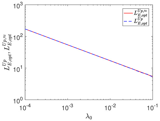
Figure 4. (Color online.) The optimal upper bound of expected queries $L_{E,opt}^{Up}\left({\lambda }_0\right)$ and its approximation $L_{E,opt}^{Up,\approx }\left({\lambda }_0\right)$ as functions of the lower bound ${\lambda }_0\in \left[{10}^{-4},{10}^{-1}\right]$ of the fraction of target items. The blue dashed and red solid curves represent $L_{E,opt}^{Up}\left({\lambda }_0\right)$ and $L_{E,opt}^{Up,\approx }\left({\lambda }_0\right)$, respectively.

6. Conclusions

In summary, we have analyzed the performance and optimized the parameters of the OFPQS algorithm. We derived the least number of iterations (denoted by $l_{opt}$) of the OFPQS algorithm to ensure the success probability for a given lower bound of the fraction of target items no less than $1-{\delta }^2$. Moreover, all extreme points as well as the minimum value of the success probability of the OFPQS algorithm were analyzed. In addition, we calculated the upper bound of expected queries of repeatedly executing the OFPQS algorithm to find a target item, and further analytically derived the optimal parameter that minimizes this upper bound. Compared with the minimum number of iterations given by [20], our optimal number of iterations $l_{opt}$ has a significant reduction, e.g., when $\delta =0.8$, almost a quarter of iterations can be saved. Our study can provide a guideline for the research and application of the OFPQS algorithm.

References

- Grover, L.K. A fast quantum mechanical algorithm for database search. In Proceedings of the Twenty-Eighth Annual ACM Symposium on Theory of Computing; ACM: Philadelphia, PA, USA, 1996; pp. 212–219. [Google Scholar]
- Grover, L.K. Quantum computers can search arbitrarily large databases by a single query. Phys. Rev. Lett. 1997, 79, 4709. [Google Scholar] [CrossRef]
- Bennett, C.H.; Bernstein, E.; Brassard, G.; Vazirani, U. Strengths and weaknesses of quantum computing. SIAM J. Comput. 1997, 26, 1510. [Google Scholar] [CrossRef]
- Boyer, M.; Brassard, G.; Høyer, P.; Tapp, A. Tight bounds on quantum searching. Fortschr. Phys. 1998, 46, 493. [Google Scholar] [CrossRef]
- Zalka, C. Grover’s quantum searching algorithm is optimal. Phys. Rev. A 1999, 60, 2746. [Google Scholar] [CrossRef]
- Grover, L.K.; Radhakrishnan, J. Is partial quantum search of a database any easier? In Proceedings of the Seventeenth Annual ACM Symposium on Parallelism in Algorithms and Architectures; ACM: Las Vegas, NV, USA, 2005; pp. 186–194. [Google Scholar]
- Brassard, G. Searching a quantum phone book. Science 1997, 275, 627. [Google Scholar] [CrossRef]
- Nielsen, M.A.; Chuang, I.L. Quantum Computation and Quantum Information, 2nd ed; Cambridge University Press: Cambridge, UK, 2010. [Google Scholar]
- Brassard, G.; Høyer, P. An exact quantum polynomial-time algorithm for Simon’s problem. In Proceedings of the Fifth Israel Symposium on the Theory of Computing Systems; IEEE Computer Society: Washington, DC, USA, 1997; pp. 12–23. [Google Scholar]
- Grover, L.K. Quantum computers can search rapidly by using almost any transformation. Phys. Rev. Lett. 1998, 80, 4329. [Google Scholar] [CrossRef]
- Brassard, G.; Høyer, P.; Tapp, A. Quantum counting. In International Colloquium on Automata, Languages, and Programming; Larsen, K.G., Skyum, S., Winskel, G., Eds.; Springer: Berlin, Germany, 1998; pp. 820–831. [Google Scholar]
- Brassard, G.; Høyer, P.; Mosca, M.; Tapp, A. Quantum amplitude amplification and estimation. In Quantum Computation and Information; Lomonaco, S.J., Jr., Brandt, H.E., Eds.; AMS: Providence, RI, USA, 2002; pp. 53–74. [Google Scholar]
- Long, G.L.; Li, Y.S.; Zhang, W.L.; Niu, L. Phase matching in quantum searching. Phys. Lett. A 1999, 262, 27. [Google Scholar] [CrossRef]
- Høyer, P. Arbitrary phases in quantum amplitude amplification. Phys. Rev. A 2000, 62, 052304. [Google Scholar] [CrossRef]
- Long, G.-L.; Li, X.; Sun, Y. Phase matching condition for quantum search with a generalized initial state. Phys. Lett. A 2002, 294, 143. [Google Scholar] [CrossRef]
- Li, P.; Li, S. Phase matching in Grover’s algorithm. Phys. Lett. A 2007, 366, 42. [Google Scholar] [CrossRef]
- Grover, L.K. Fixed-point quantum search. Phys. Rev. Lett. 2005, 95, 150501. [Google Scholar] [CrossRef] [PubMed]
- Chakraborty, S.; Radhakrishnan, J.; Raghunathan, N. Bounds for error reduction with few quantum queries. In Approximation, Randomization and Combinatorial Optimization. Algorithms and Techniques; Springer: Berlin, Germany, 2005; pp. 245–256. [Google Scholar]
- Tulsi, T.; Grover, L.K.; Patel, A. A new algorithm for fixed point quantum search. Quantum Inf. Comput. 2006, 6, 483. [Google Scholar]
- Yoder, T.J.; Low, G.H.; Chuang, I.L. Fixed-point quantum search with an optimal number of queries. Phys. Rev. Lett. 2014, 113, 210501. [Google Scholar] [CrossRef] [PubMed]
- Toyama, F.M.; van Dijk, W.; Nogami, Y.; Tabuchi, M.; Kimura, Y. Multiphase matching in the Grover algorithm. Phys. Rev. A 2008, 77, 042324. [Google Scholar] [CrossRef]
- Toyama, F.M.; Kasai, S.; van Dijk, W.; Nogami, Y. Matched-multiphase Grover algorithm for a small number of marked states. Phys. Rev. A 2009, 79, 014301. [Google Scholar] [CrossRef]
- Mason, J.; Handscomb, D. Chebyshev Polynomials; CRC Press: Boca Raton, FL, USA, 2002. [Google Scholar]
- Zwillinger, D. CRC Standard Mathematical Tables and Formulae; CRC Press: Boca Raton, FL, USA, 2011. [Google Scholar]
© 2019 by the authors. Licensee MDPI, Basel, Switzerland. This article is an open access article distributed under the terms and conditions of the Creative Commons Attribution (CC BY) license (http://creativecommons.org/licenses/by/4.0/).