MPC for Optimized Energy Exchange between Two Renewable-Energy Prosumers

Abstract

Renewable energy and information technologies are changing electrical energy distribution, favoring a move towards distributed production and trading between many buyers and sellers. There is new potential for trading between prosumers, entities which both consume and produce energy in small quantities. This work explores the optimization of energy trading between two prosumers, each of which consists of a load, renewable supply, and energy storage. The problem is described within a model predictive control (MPC) framework, which includes a single objective function to penalize undesirable behavior, such as the use of energy from a utility company. MPC integrates future predictions of supply and demand into current dispatch decisions. The control system determines energy flows between each renewable supply and load, battery usage, and transfers between the two prosumers. At each time step, future predictions are used to create an optimized power dispatch strategy between the system prosumers, maximizing renewable energy use. Modeling results indicate that this coordinated energy sharing between a pair of prosumers can improve their overall renewable energy penetration. For one specific choice of prosumers (mixed residential–commercial) penetration is shown to increase from 71% to 84%.

1. Introduction

Electric power grids are currently undergoing a transition from large centralized power stations to distributed generation, which includes significant renewable components [1]. Utilizing a high percentage of intermittent renewable energy creates new engineering problems, requiring greater flexibility from controllable power sources and large-scale energy storage systems. Information technology is also shaping changes to the energy sector, allowing for automated and reliable tracking of transactions between many buyers and sellers [2]. The new ability for small prosumers to trade directly with each other creates potential to improve renewable energy utilization. This work explores an optimal dispatch algorithm that controls all energy flows within two prosumers (small scale producers and consumers, such as homes with rooftop PV) and determines when they should share energy.

1.1. Microgrids

A microgrid is a small electrical network that includes loads, sources, and possibly storage, and can trade power with the larger electrical grid or, at times, operate in islanded mode. For example, a microgrid installation at the University of California San Diego can generate more than 90% of the electricity used on campus annually with wind and solar power, saving more than $800,000 per month [3]. There are several areas of microgrid research that support the overall goal of maximizing the usage of locally produced (often renewable) energy. A microgrid with significant renewable components requires careful frequency and voltage control, AC/DC conversion, and other electrical considerations [4]. Optimal power point tracking can be applied to get the most energy transfer possible from a turbine or PV system [5]. Correctly sizing the renewable components for a given load is another microgrid research topic. For example, researchers have studied the problem of sizing a hybrid solar/wind system with battery storage as a multiobjective optimization, using a genetic algorithm (GA) to minimize both annual system cost as well as the probability of losing power [6]. Researchers have also considered optimizing the control algorithms for island microgrid operations, with management of battery storage and diesel generation using forecasting [7]. Previous work by the authors reported on studies with a control scheme for a microgrid with battery and thermal storage, and a methodology for sizing these components [8,9].

If microgrids can trade energy with one another, this provides another opportunity for improving the overall renewable penetration as well as the value of each microgrid. In this case, when one microgrid has excess energy it has the option to transfer this energy to microgrids with an energy deficit. Blockchain technology for automatically tracking such transactions has recently been developed [10]. A microgrid network in Brooklyn, New York applies this technology, allowing members to efficiently manage and record energy transactions within the local network [11]. A summary of case studies involving peer-to-peer energy sharing is provided by [12]. The concept of optimizing the overall performance of a network of microgrids is relatively new in the literature. A framework for such a network can be studied as a convex optimization problem combining transactions and distributed energy production costs, using algorithms such as alternating direction method of multipliers (ADMM) to maximize renewable penetration while minimizing costs [13]. Other researchers have created an energy sharing structure to integrate prosumers into an energy sharing zone with an internal pricing model based on supply and demand ratio for renewable energy [14]. A model predictive control (MPC) framework is applied to a microgrid network to optimize the scheduling of power exchange between members as well as control local energy storage systems using forecasts of load, supply, and prices [15].

1.2. Outline and Scope of This Work

The approach in this work is to develop a single dispatching scheme that coordinates a pair of prosumers to optimize their overall renewable energy penetration. This is unique in that it utilizes future predictions of supply and load for both prosumers and creates a single objective function to optimize. The control scheme determines the flows within each prosumer, as well as the energy trading between them, to optimize an objective, effectively turning the two prosumers into a single operating unit. This is conceived here as a centralized approach that could be implemented by a third party who receives data from both prosumers, as well as weather forecasts, and transmits real-time energy allocation instructions back to the prosumers. Future work will focus on a decentralized version of this concept, operating in a manner like the prosumer network in New York mentioned earlier [11]. The scheme would also require cooperation from the local utility company, in terms of reasonable tariffs for utilizing their infrastructure and for purchasing excess energy from the prosumers. The two prosumers can be pre-existing entities (prosumers) that are ideally selected to be complementary, such that one is likely to have an energy deficit when the other has a surplus. The proposed control scheme enables better overall penetration for the two prosumers and reduces the exchanges between them and external providers. The behavior of the algorithm can be modified through the objective function, by including terms that reflect battery storage lifetime, for example.

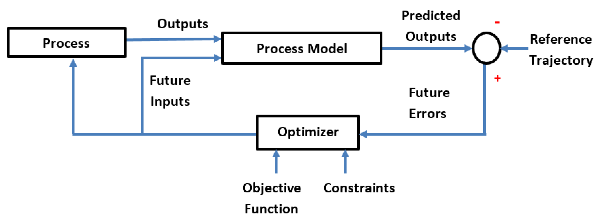
1.3. Model Productive Control

Model predictive control (MPC) refers to techniques that utilize models of a process and incorporate future predictions of performance and external variables to systematically determine control signals by minimizing an objective function at each time step [16]. These algorithms predict future process behavior and choose a control sequence to optimize an objective function based on these predictions. The initial value of this control sequence is retained before advancing the prediction window into the future for the next time step. Applications of MPC include industrial control of robots, servo motors, steam generators, and control of anesthesia delivery [17]. As well as having the ability to utilize available forecasting data, MPC can efficiently incorporate constraints and manage multiple control variables. MPC does have a large computational burden (the optimization) at each time step, although this is only a problem for applications that require high-speed sampling. A generic MPC schematic is illustrated in Figure 1, where a process model predicts future outputs based on previous inputs/outputs and optimized future control signals.

MPC is frequently applied to power delivery systems, especially those that involve renewable sources and distributed generation. For example, MPC is used in maximum power point tracking for DC power systems, to manage the fluctuating output from a PV array connected to a constant DC bus [18]. Active and reactive power disturbances that occur within combined wind-turbine and battery microgrids can also be controlled by MPC, while maximizing power delivery from the turbines [19]. These algorithms have also been used to mitigate disturbances caused by errors in weather forecasting models in a distributed generation system [20].

1.4. Case Study

Figure 2 below illustrates the main components of the two prosumers used in this study and power flows between them. These two prosumers are envisioned as two prosumers within a larger network of prosumers. The structure of both prosumers is the same, consisting of a load, renewable energy supply, battery storage, and connections to other sources of power, such as the other prosumers in the larger network and/or a retail energy supplier. Transactions between the two prosumers are shown as power flows through the peer-to-peer transactions block.

The differences between the prosumers are captured in the two load profiles and the renewable energy profiles, the example used throughout this work imagines one load as residential and the other as commercial, although the system applies to any two loads that are complementary to one another. The residential and commercial load profiles are modeled based on real data, and renewable energy resource (RER) supplies are based on typical meteorological year (TMY) weather data and models for PV and wind turbines. The modeling presented here does not include currents or voltages, just discrete hourly energy flows. Variable energy pricing is not modeled, although the MPC objective function contains parameters that could depend on energy prices. Although there are several MPC formulations possible, here, a state space approach is used because it allows for handling many variables easily.

The cost function is formulated as a constrained quadratic, whose complexity depends on the number of variables and the length of the control horizon. Referring again to Figure 2, it is possible to consider MPC operation with or without the energy sharing. This can be easily achieved by adjusting constraint parameters within the algorithm. This allows for exploration of the potential benefit of coupling two prosumers within a larger network of prosumers. Energy sharing between the two coupled prosumers is prioritized over energy sharing with other prosumers in the network.

2. Problem Formulation

The MPC algorithm is designed to maximize the use of renewable power for the two loads, minimizing the trading that occurs with the rest of the network or other retail energy suppliers. This means that the algorithm seeks to isolate the coupled prosumers as much as possible from the rest of the energy network. The following subsections define the MPC problem, including a battery storage model, state-space formulation, objective function, a reference trajectory based on forecast information, and all system constraints.

2.1. Battery Storage

Using k to represent hourly time steps ($k=1,2,3,\cdots )$, the two battery states of charge $SO{C}_R\left(k\right)$ and $SO{C}_C\left(k\right)$, both in kWh, are combined into a single vector,

$$x_m\left(k\right)=\left[\begin{array}{c}SO{C}_R\left(k\right)\\ SO{C}_C\left(k\right)\end{array}\right].$$

This vector will become part of the state-space model, and it is used to construct a recursive matrix algebra update for the batteries, with the following equation and definitions.

$$x_m\left(k+1\right)=x_m\left(k\right)+b_{m}u\left(k\right),$$

(1)

$$u\left(k\right)={[P_{2R},P_{2C},P_{3R},P_{3C},P_{4R},P_{4C},P_{RC},P_{CR},P_{BRC},P_{BCR}]}^{\top },$$

$$b_m=\left[\begin{array}{cccccccccc}0& 0& {\eta }_C& 0& -{\eta }_D& 0& 0& 0& 0& 0\\ 0& 0& 0& {\eta }_C& 0& {-\eta }_D& 0& 0& 0& 0\end{array}\right].$$

In these definitions, ${\eta }_C$ and ${\eta }_D$ are the charging and discharging efficiencies for energy transfers to the battery $P_{3R}$,$P_{3C}$ and from the battery $P_{4R}$,$P_{4C}$, respectively. The vector $u\left(k\right)$ is defined as the control vector for the system, and it contains all the energy flows that the algorithm must choose at each time step. These flows are all functions of k, although this is not shown to simplify the expressions.

2.2. State-Space Formulation

To develop a state-space representation of the system, it is first necessary to define an objective function and system outputs.

Table 1. System outputs and objective terms.

System Outputs	Objective Function Terms	Description
$y_{mR}=C_1[P_{2R}+P_{4R}+P_{CR}+P_{BCR}]$	$J_{1R}=C_1^2{P}_{1R}^2={[C_1{P}_{LR}-y_{mR}]}^2$	Energy purchased from other network
$y_{mC}=C_1[P_{2C}+P_{4C}+P_{RC}+P_{BRC}]$	$J_{1C}=C_1^2{P}_{1C}^2={[C_1{P}_{LR}-y_{mR}]}^2$	prosumers or retail suppliers
$y_{aR}=C_2(P_{3R}+P_{4R})$	$J_{2}R=C_2^2{(P_{3R}+P_{4R})}^2=y_{aR}^2$	Charging and discharging energy
$y_{aC}=C_2(P_{3C}+P_{4C})$	$J_{2}C=C_2^2{(P_{3C}+P_{4C})}^2=y_{aC}^2$	transfer to battery
$y_{bR}=C_3{P}_{5R}$	$J_{3R}=C_3^2{P}_{5R}^2=y_{bR}^2$	Energy sold to other network prosumers
$y_{bC}=C_3{P}_{5C}$	$J_{3C}=C_3^2{P}_{5C}^2=y_{bC}^2$
$y_{dR}=C_4{P}_{RC}$	$J_{4R}=C_{4R}^2{P}_{RC}^2=y_{dR}^2$	Energy transferred from the residential renewable energy resource (RER)
$y_{dC}=C_4{P}_{CR}$	$J_{4C}=C_{4C}^2{P}_{CR}^2=y_{dC}^2$	supply to the commercial load and vice versa
$y_{eR}=C_5{P}_{BRC}$	$J_{5R}=C_5^2{P}_{BRc}^2=y_{eR}^2$	Energy transferred from the residential
$y_{eC}=C_5{P}_{BCR}$	$J_{5C}=C_5^2{P}_{BCR}^2=y_{eC}^2$	battery to the commercial load and vice versa

Where R—residential prosumer and C—commercial prosumer.

organizes the definitions of objective function terms and corresponding outputs. Each term represents a system energy component that can be penalized by selection of corresponding weighting terms, $C_1$ to $C_5$. Note that renewable energy that is consumed directly by the loads is not penalized, whereas there are objective terms for externally supplied power ($J_{1R},J_{1C}$), energy into and out of the batteries ($J_{2R},J_{2C}$), energy flows to other network prosumers ($J_{3R},J_{3C}$), RER flows between the coupled prosumers ($J_{4R},J_{4C}$), and battery flows between the coupled prosumers ($J_{5R},J_{5C}$). Constants $C_1$ to $C_5$ serve as weighting parameters that can modify the relative significance of each objective term. The definition of the terms ($J_{1R}$) relies on the constraint that the load must be completely satisfied at each time step ($P_{1R}=P_{LR}-P_{2R}-P_{4R}-P_{CR}-P_{BCR}$). The same constraint holds for the commercial prosumer.

To formulate the state-space model, we define the ten system outputs listed in Table 1 which are combined as a single output vector $y\left(k\right)$. The system input $x\left(k\right)$ is constructed from $x_m\left(k\right)$ and $y\left(k\right)$. The following expressions summarize these relationships.

$$y(k+1)=[y_{mR}\left(k\right),y_{mC}\left(k\right),y_{aR}\left(k\right),y_{aC}\left(k\right),y_{bR}\left(k\right),...$$

$$y_{bC}\left(k\right),y_{dR}\left(k\right),y_{dC}\left(k\right),y_{eR}\left(k\right),y_{eC}{\left(k\right)]}^{\top },$$

$$x\left(k\right)=\left[\begin{array}{c}{x}_m\left(k\right)\\ y\left(k\right)\end{array}\right].$$

$$x(k+1)=Ax\left(k\right)+Bu\left(k\right),$$

(2)

$$y\left(k\right)=Cx\left(k\right),$$

where

$$A=\left[\begin{array}{cc}{I}_{2\times 2}& 0_{2\times 10}\\ 0_{10\times 2}& 0_{10\times 10}\end{array}\right],$$

$$B=\left[\begin{array}{cccccccccc}0& 0& {\eta }_c& 0& -{\eta }_D& 0& 0& 0& 0& 0\\ 0& 0& 0& {\eta }_C& 0& -{\eta }_D& 0& 0& 0& 0\\ C_1& 0& 0& 0& C_1& 0& 0& C_1& 0& 0\\ 0& C_1& 0& 0& 0& C_1& C_1& 0& 0& 0\\ C_3& 0& C_3& 0& 0& 0& C_3& 0& 0& 0\\ 0& C_3& 0& C_3& 0& 0& 0& C_3& 0& 0\\ 0& 0& C_2& 0& C_2& 0& 0& 0& 0& 0\\ 0& 0& 0& C_2& 0& C_2& 0& 0& 0& 0\\ 0& 0& 0& 0& 0& 0& C_4& 0& 0& 0\\ 0& 0& 0& 0& 0& 0& 0& C_4& 0& 0\\ 0& 0& 0& 0& 0& 0& 0& 0& C_5& 0\\ 0& 0& 0& 0& 0& 0& 0& 0& 0& C_5\end{array}\right],$$

and

$$C=\left[\begin{array}{cc}{0}_{10\times 2}& I_{10\times 10}\end{array}\right].$$

2.3. MPC Objective Function and Reference Trajectory

The MPC objective function is defined at each time step by summing all ten terms in Table 1. The function looks forward to a time horizon defined by $N_p$, summing energy terms over a selected time interval according to

$$J\left(k\right)={\sum }_{i=k}^{k+N_p}{\sum }_{q=1}^5\left[J_{qR}\left(i\right)+J_{qC}\left(i\right)\right].$$

(3)

To develop an expression for $J\left(k\right)$ that can be expressed as a quadratic, we define

$$\begin{array}{c}Y\left(k\right)={[Y^T\left(k\right),Y^T(k+\left.1\right|k),...,Y^T(k+N_p-\left.1\right|k)]}^T,\hfill \end{array}$$

where the notation $y(k+i|k)$ represents the predicted value of y at step i associated with sampling time k.

Using the same notation, future predictions for residential and commercial loads are represented by $P_{LR}(k+i|k)$ and $P_{LC}(k+i|k)$, respectively. These could be generated from historical data, models for human behavior, weather forecasts, etc. Similarly, future predictions for residential and commercial RER outputs are represented by $P_{RE{R}_R}(k+i|k)$ and $P_{RE{R}_C}(k+i|k)$, respectively, as would be generated from weather forecasts and models for the various hardware components involved in renewable power generation. All the predicted quantities, for each time step into the future up to the prediction horizon $N_p$, are combined into a single reference trajectory vector $R\left(k\right)$, given by

$$R\left(k\right)=\left[\begin{array}{c}{C}_1{P}_{LR}\left(k\right)\\ C_1{P}_{LC}\left(k\right)\\ C_3{P}_{RE{R}_R}\left(k\right)\\ C_3{P}_{RE{R}_C}\left(k\right)\\ 0_{6\times 1}\\ ⋮\\ C_1{P}_{LR}(k+N_p|k)\\ C_1{P}_{LC}(k+N_p|k)\\ C_3{P}_{RE{R}_R}(k+N_p|k)\\ C_3{P}_{RE{R}_C}(k+N_p|k)\\ 0_{6\times 1}\end{array}\right].$$

(4)

The output vector $Y\left(k\right)$ should follow this reference, and the minimization of the MPC objective can now be re-expressed in quadratic form:

$$minJ\left(k\right)=min{(Y\left(k\right)-R\left(k\right))}^{\top }(Y\left(k\right)-R\left(k\right)).$$

(5)

2.4. System Constraints

There are two main equality constraints in the system model, such that the power total flows into the loads meet those loads exactly at each time interval,

$$P_{LR}\left(k\right)=P_{2R}\left(k\right)+P_{4R}\left(k\right)+P_{1R}\left(k\right)+P_{CR}\left(k\right)+P_{BCR}\left(k\right),$$

(6)

$$P_{LC}\left(k\right)=P_{2C}\left(k\right)+P_{4C}\left(k\right)+P_{1C}\left(k\right)+P_{RC}\left(k\right)+P_{BRC}\left(k\right).$$

(7)

The power flows that form the control vector $u\left(k\right)$, must meet various inequality constraints. Each of these flows is non-negative and each has an upper bound. In addition, transfers from the RER and battery to the residential load cannot exceed the load

$$P_{2R}\left(k\right)+P_{4R}\left(k\right)+P_{CR}\left(k\right)+P_{BCR}\left(k\right)\le P_{LR}\left(k\right),$$

(8)

$$P_{2C}\left(k\right)+P_{4C}\left(k\right)+P_{RC}\left(k\right)+P_{BRC}\left(k\right)\le P_{LC}\left(k\right).$$

(9)

Also, the three power flows from the RER supply cannot exceed the total available RER output at any time.

$$P_{2R}\left(k\right)+P_{3R}\left(k\right)+P_{RC}\left(k\right)\le P_{RE{R}_R}\left(k\right),$$

(10)

$$P_{2C}\left(k\right)+P_{3C}\left(k\right)+P_{CR}\left(k\right)\le P_{RE{R}_C}\left(k\right).$$

(11)

The power flows $P_{1R}\left(k\right)$ and $P_{1C}\left(k\right)$ are bounded according to

$$0\le P_{1R}\left(k\right)\le P_{1R}^{max},$$

(12)

$$0\le P_{1C}\left(k\right)\le P_{1C}^{max}.$$

(13)

Due to equality constraints, Equations (8) and (9), these can be rewritten as

$$P_{2R}\left(k\right)+P_{4R}\left(k\right)+P_{CR}\left(k\right)+P_{BCR}\left(k\right)\ge P_{1R}^{max}-P_{LR}\left(k\right),$$

(14)

$$P_{2C}\left(k\right)+P_{4C}\left(k\right)+P_{RC}\left(k\right)+P_{BRC}\left(k\right)\ge P_{1C}^{max}-P_{LC}\left(k\right).$$

(15)

The inequality constraints can now be summarized in a single expression

$${\gamma }_1\ge M_{1}u\left(k\right),$$

(16)

where ${\gamma }_1={[{\gamma }_R,{\gamma }_C]}^{\top }$, the inequality is taken elementwise, and ${\gamma }_R$ and ${\gamma }_C$ are defined as

$${\gamma }_R=\left[\begin{array}{c}{P}_{RE{R}_R}\left(k\right)\\ P_{2R}^{max}\\ P_{3R}^{max}\\ P_{4R}^{max}\\ P_{RC}^{max}\\ P_{BRC}^{max}\\ P_{1R}^{max}-P_{LR}\left(k\right)\\ P_{LR}\left(k\right)\\ 0_{6\times 1}\end{array}\right],{\gamma }_C=\left[\begin{array}{c}{0}_{6\times 1}\\ P_{RE{R}_C}\left(k\right)\\ P_{2C}^{max}\\ P_{3C}^{max}\\ P_{4C}^{max}\\ P_{CR}^{max}\\ P_{BCR}^{max}\\ P_{1C}^{max}-P_{LC}\left(k\right)\\ P_{LC}\left(k\right)\end{array}\right].$$

Furthermore, $M_1={[M_R,M_C]}^{\top }$, where $M_R$ and $M_C$ are defined as

$$M_R=\left[\begin{array}{cccccccccc}1& 0& 1& 0& 0& 0& 1& 0& 0& 0\\ -1& 0& -1& 0& 0& 0& -1& 0& 0& 0\\ 1& 0& 0& 0& 0& 0& 0& 0& 0& 0\\ -1& 0& 0& 0& 0& 0& 0& 0& 0& 0\\ 0& 0& 1& 0& 0& 0& 0& 0& 0& 0\\ 0& 0& -1& 0& 0& 0& 0& 0& 0& 0\\ 0& 0& 0& 0& 1& 0& 0& 0& 0& 0\\ 0& 0& 0& 0& -1& 0& 0& 0& 0& 0\\ 0& 0& 0& 0& 0& 0& 1& 0& 0& 0\\ 0& 0& 0& 0& 0& 0& -1& 0& 0& 0\\ 0& 0& 0& 0& 0& 0& 0& 1& 0& 0\\ 0& 0& 0& 0& 0& 0& 0& -1& 1& 0\\ -1& 0& 0& 0& -1& 0& 0& -1& 0& -1\\ 1& 0& 0& 0& 1& 0& 0& 1& 0& 1\end{array}\right],$$

$$M_C=\left[\begin{array}{cccccccccc}0& 1& 0& 1& 0& 0& 0& 1& 0& 0\\ 0& -1& 0& -1& 0& 0& 0& -1& 0& 0\\ 0& 1& 0& 0& 0& 0& 0& 0& 0& 0\\ 0& -1& 0& 0& 0& 0& 0& 0& 0& 0\\ 0& 0& 0& 1& 0& 0& 0& 0& 0& 0\\ 0& 0& 0& -1& 0& 0& 0& 0& 0& 0\\ 0& 0& 0& 0& 0& 1& 0& 0& 0& 0\\ 0& 0& 0& 0& 0& -1& 0& 0& 0& 0\\ 0& 0& 0& 0& 0& 0& 0& 1& 0& 0\\ 0& 0& 0& 0& 0& 0& 0& -1& 0& 0\\ 0& 0& 0& 0& 0& 0& 0& 0& 0& 1\\ 0& 0& 0& 0& 0& 0& 0& 0& 0& -1\\ 0& -1& 0& 0& 0& -1& -1& 0& -1& 0\\ 0& 1& 0& 0& 0& 1& 1& 0& 1& 0\end{array}\right].$$

The constraints are applied to the predicted control flows at each future time step, using the following definition of the predictive control vector, where $N_C$ is the control horizon.

The constraints are then applied at each time step,

$$\left[\begin{array}{c}{\gamma }_1\left(k\right)\\ {\gamma }_1\left(k\right)\\ ⋮\\ {\gamma }_1\left(k\right)\end{array}\right]\ge U\left(k\right)\left[\begin{array}{ccc}{M}_1& \cdots & 0\\ ⋮& \ddots & ⋮\\ 0& \cdots & M_1\end{array}\right],$$

(17)

where ${\overline{\gamma }}_1\left(k\right)=\left[\begin{array}{c}{\gamma }_1\left(k\right)\\ {\gamma }_1\left(k\right)\\ ⋮\\ {\gamma }_1\left(k\right)\end{array}\right]$ and ${\overline{M}}_1=\underset{N_c}{\underbrace{\left[\begin{array}{ccc}{M}_1& \cdots & 0\\ ⋮& \ddots & ⋮\\ 0& \cdots & M_1\end{array}\right]}}$.

The predicted values of the state of charge can now be written as

$$x_m(k+i|k)=x_m\left(k\right)+b_m\sum _{j=k}^{j\le k+i-1}u\left(j\right).$$

(18)

By defining the predictive state of charge $X_m$ (k) as

$$X_m\left(k\right)\triangleq \left[\begin{array}{c}{x}_m\left(k\right)\\ x_m(k+1|k)\\ x_m(k+N_c-1|k)\end{array}\right],$$

(19)

we can write

$$X_m\left(k\right)=\left[\begin{array}{c}{I}_{2\times 2}\\ I_{2\times 2}\\ ⋮\\ I_{2\times 2}\end{array}\right]x_m\left(k\right)+B_{m}U\left(k\right),B_m=\left[\begin{array}{cccc}{b}_m& 0& \cdots & 0\\ b_m& b_m& \ddots & ⋮\\ ⋮& \ddots & 0\\ b_m& b_m& \cdots & b_m\end{array}\right].$$

Since each storage system state of charge is constrained to be between upper and lower limits, this can be applied to each of the predicted values $x_m(k+i|k)$ in the predictive state of charge. The constraints can then be represented in one inequality $\overline{\gamma }\ge \overline{M}U\left(k\right)$ as

$$\left[\begin{array}{c}{\overline{\gamma }}_1\\ {\overline{\gamma }}_2\end{array}\right]\ge \left[\begin{array}{c}u\left(k\right)\\ u(k+1|k)\\ u(k+N_c-1|k)\end{array}\right]\left[\begin{array}{c}{\overline{M}}_1\\ {\overline{M}}_2\end{array}\right],$$

(20)

where ${\overline{\gamma }}_2$ and ${\overline{M}}_2$ are defined as

$${\overline{\gamma }}_2=\left[\begin{array}{cc}\left(x_m\left(k\right)-\left[\begin{array}{c}{B}_{CR}^{min}\\ B_{CC}^{min}\end{array}\right]\right)& \left[\begin{array}{c}{I}_{2\times 2}\\ I_{2\times 2}\\ ⋮\\ I_{2\times 2}\end{array}\right]\\ \left(\left[\begin{array}{c}{B}_{CR}^{min}\\ B_{CC}^{min}\end{array}\right]-x_m\left(k\right)\right)& \left[\begin{array}{c}{I}_{2\times 2}\\ I_{2\times 2}\\ ⋮\\ I_{2\times 2}\end{array}\right]\end{array}\right],{\overline{M}}_2=\left[\begin{array}{c}-B_m\\ B_m\end{array}\right].$$

2.5. MPC Algorithm

Given the system model, Equation (2); the objective function, Equation (3); and the constraint equation on Equation (16), it is possible to develop the MPC algorithm, as outlined by Wang [21]. First, the following MPC gains are formed:

$$F={\left[\begin{array}{ccccc}{\left(CA\right)}^{\top },& {\left(C{A}^2\right)}^{\top },\cdots & \cdots & \cdots & {\left(C{A}^{N_p}\right)}^{\top }\end{array}\right]}^{\top },$$

$$=\left[\begin{array}{cccc}\left(CA\right)& 0& \cdots & 0\\ \left(CAB\right)& \left(CB\right)& & 0\\ ⋮& & \ddots & ⋮\\ (C{A}^{N_p-1}B& (C{A}^{N_p-2}B& \cdots & (C{A}^{N_p-N_c}B\end{array}\right],$$

and

$$E={\varphi }^{\top }\varphi ,H={(Fx\left(k\right)-R\left(k\right))}^{\top }\varphi .$$

Using these definitions, the predicted output vector becomes $Y\left(k\right)=Fx\left(k\right)+\varphi U\left(k\right)$. This allows the quadratic form of the objective in Equation (5) to be rewritten as

$$J\left(k\right)={(Fx\left(k\right)-R\left(k\right))}^{\top }(Fx\left(k\right)-R\left(k\right))+2{(Fx\left(k\right)-R\left(k\right))}^{\top }\varphi U\left(k\right)+U{\left(k\right)}^{\top }{\varphi }^{\top }\varphi U\left(k\right).$$

(21)

The minimization of the objective function can now be expressed using terms that depend only on $U\left(k\right)$,

$$minJ\left(k\right)=min[2{(Fx\left(k\right)-R\left(k\right))}^{\top }\varphi U\left(k\right)+U{\left(k\right)}^{\top }{\varphi }^{\top }\varphi U\left(k\right)].$$

(22)

Using Matlab© quadratic programming optimization routine at Equation (21) is solved under the constraints in Equation (16). A receding horizon control is implemented by keeping $u\left(k\right)$, the first 10 elements $U\left(k\right)$. All system states, inputs, and outputs are then updated using $u\left(k\right)$ and state-space, Equation (2), for the next time $k=k+1$, and the process is then repeated for the next time step.

3. Simulation Results

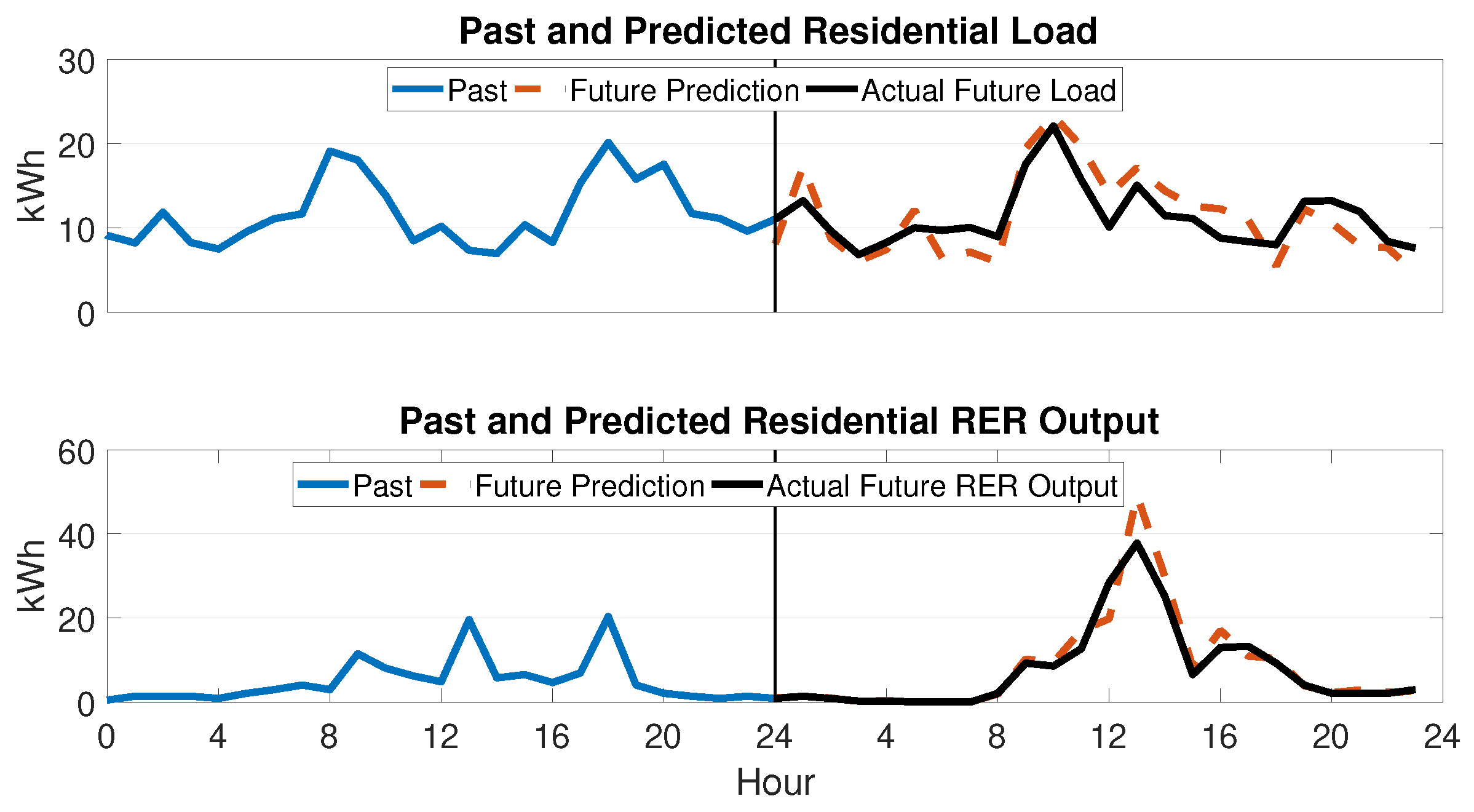
3.1. Load and Supply Forecasting

To evaluate this MPC approach requires realistic data for residential and commercial loads, RER supply profiles for the locations of these loads, and methods for forecasting these four quantities into the future. The load profiles used are derived from residential apartment meter readings and a model for a commercial-kitchen electrical load, resulting in hourly demand $P_{LR}\left(k\right)$ and $P_{L}C\left(k\right)$ for one year [6]. At each hour k, the demand forecasts $P_{LR}(k+i|k)$ and $P_{LC}(k+i|k)$ for $i=1,\dots ,N_P$ are selected randomly and uniformly from 60% to 140% of the actual future demand, where $N_P$ is the predicted horizon of future load demand and equal to 24 h.

The RER profiles $P_{RE{R}_R}$ and $P_{RE{R}_C}$ are each created as a mix of wind and solar power, using wind turbines 3 ${\mathrm{m}}^2$ swept area per turbine), fixed position solar panels 2 ${\mathrm{m}}^2$ per panel), and a model that converts TMY data for Ohio into hourly turbine and solar PV output [6]. The residential RER system has 1 turbine, 150 panels, and 220 kWh battery capacity; and the commercial RER system has 2 turbines, 120 panels, and 180 kWh battery capacity. The RER output forecasts at each hour k, $P_{RE{R}_R}(k+i|k)$ and $P_{RE{R}_C}(k+i|k)$ for $i=1,\dots ,N_P$ are selected randomly and uniformly from 80% to 120% of the actual RER powers, where $N_P$ is the predict horizon of future supply and equal to 24 h.

Figure 3 and Figure 4 show examples of demand and supply profiles for the residential and commercial systems. The vertical line in each subplot indicates current time k, corresponding to midnight, with one day of past (historical) values to the left and one day of future forecasted values to the right. Actual future load and supply (which would not be known in a real application) are also shown to illustrate forecasting error.

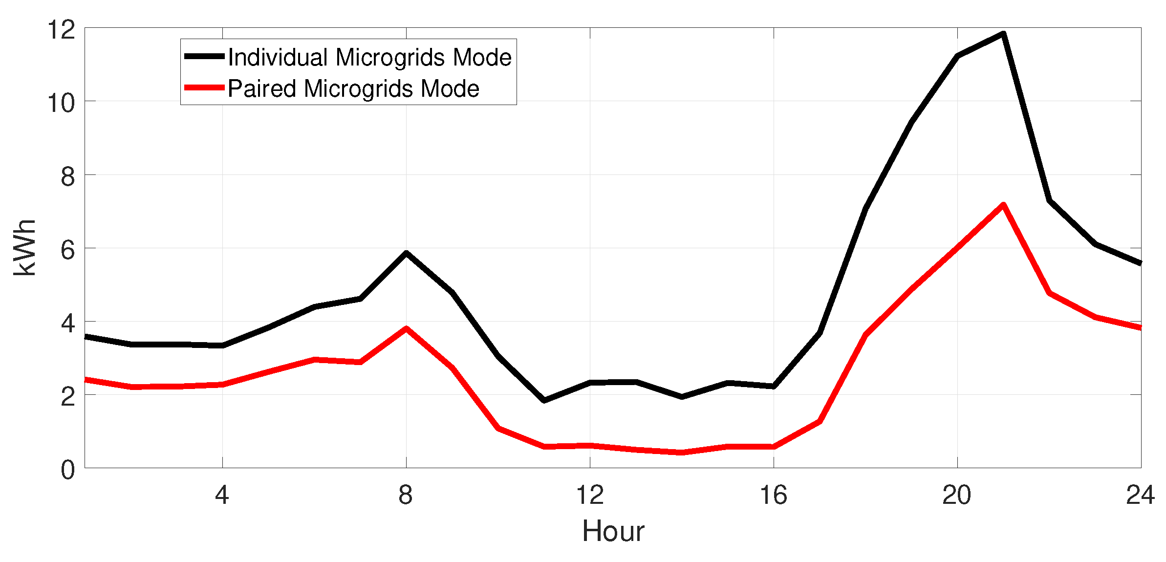
3.2. Performance Benefit of Prosumer Pairing

The MPC algorithm can be operated in two ways, with or without sharing between the paired prosumers. To run the algorithm in unshared mode, the parameters $P_{RC}^{max}$, $P_{CR}^{max}$, $P_{BCR}^{max}$, and $P_{BRC}^{max}$ are all set to zero, which prevents the MPC algorithm from sharing energy between the prosumers. By running the algorithm for the full year, sharing and unsharing, comparisons can be made between the two scenarios to illustrate the benefits of sharing/pairing. For the paired mode of operation, Figure 5 shows the monthly total energies that flow between the paired prosumers. This figure illustrates some seasonal activity, in that more energy is transferred from the residential to the commercial prosumer in the summer compared to the winter months. We can also see that on average, the residential prosumer has more excess energy to transfer to the commercial prosumer. The upper plot in Figure 6 shows average daily behavior for the full year, illustrating RER energy surplus (production minus load) for both prosumers. These plots indicate when each prosumer has a surplus (more RER output than load) and when each has a deficit (less RER output than load). The solar activity is apparent in these plots, showing an average surplus energy in the afternoon. There are times during the day when there are significant differences between the surplus energy available in the two prosumers. During this time, it is expected that one prosumer will be likely to transfer energy to the other prosumer, confirmed by the positive energy transfers evident in the lower plot. Clearly, the commercial prosumer transfers more energy to the residential prosumer in the morning, and vice-versa in the afternoon. This indicates how the MPC algorithm exploits differences between the two paired prosumers. Figure 7 shows total purchases from external prosumers in the network for both paired prosumers, using both modes of operation (sharing versus unshared). Clearly, the amount of energy needed from outside sources drops when the two prosumers are paired.

Table 2. Performance for both operating modes.

	Unpaired	Paired
Percentage of both loads satisfied by RER production	71%	84%
Percentage of total RER output transferred to other prosumers	39%	32%

summarizes total results for paired versus unpaired MPC operation. If the two prosumers under consideration are unpaired, the combined percentage of the loads met with RER energy is 75%, which increases to 86% when the loads are paired. In other words, a greater percentage of the RER output remains within the two prosumer paired system. The total RER output that is transferred to outside prosumers in the network decreases for the paired case.

4. Conclusions

This work describes the utility of an MPC approach for efficiently coupling two prosumers, each with their own renewable energy supply and battery storage. This builds upon earlier research which explored MPC for managing one prosumer’s energy flows to another prosumer. Here, a single MPC dispatch algorithm manages all flows internal to the paired prosumers, as well as shared energy flows between them. By exploiting differences between the two prosumers’ supply and load profiles, higher renewable energy penetration is achieved for the coupled system relative to the penetration achieved if the prosumers operate independently. An example of a residential prosumer paired with a commercial prosumer is presented to illustrate this point. The MPC approach utilizes forecasts of supply and demand, ensuring the batteries are drained prior to times of anticipated excess supply, and the batteries are full prior to times of anticipated excess demand.

Renewable penetration could be further improved by networking more than two prosumers in this manner, although the current MPC formulation may not scale easily due to the number of variables involved. One approach for scaling may be to only apply MPC to manage shared energy flows, but not flows that are internal to each prosumer.

Although this work does not explicitly consider energy pricing, the coefficients for the MPC objective function could be functions (changing in time, if necessary) of prices. The coefficients could similarly be adjusted to more precisely reflect battery efficiency and life, losses due to DC to AC conversion, physical distances between prosumers, and other electrical or economic considerations. Such approaches can further refine the potential of an MPC approach to optimized energy exchange. Future research will consider the algorithm’s performance with a smaller time-step, and modifications necessary to handle rapid fluctuations in load and supply.

References

1. Booth, S.; Barnett, J.; Burman, K.; Hambrick, J.; Westby, R. Net Zero Energy Military Installations: A Guide to Assessment and Planning; Technical Report; National Renewable Energy Lab. (NREL): Golden, CO, USA, 2010. [Google Scholar]
2. Mylrea, M.; Gourisetti, S.N.G. Blockchain for Smart Grid Resilience: Exchanging Distributed Energy at Speed, Scale and Security. In Proceedings of the Resilience Week (RWS), Wilmington, DE, USA, 18–22 September 2017; pp. 18–23. [Google Scholar]
3. Washom, B.; Dilliot, J.; Weil, D.; Kleissl, J.; Balac, N.; Torre, W.; Richter, C. Ivory tower of power: Microgrid implementation at the University of California, San Diego. IEEE Power Energy Mag. 2013, 11, 28–32. [Google Scholar] [CrossRef]
4. Díaz-González, F.; Sumper, A.; Gomis-Bellmunt, O.; Villafáfila-Robles, R. A review of energy storage technologies for wind power applications. Renew. Sustain. Energy Rev. 2012, 16, 2154–2171. [Google Scholar] [CrossRef]
5. Bizon, N. Optimal operation of fuel cell/wind turbine hybrid power system under turbulent wind and variable load. Appl. Energy 2018, 212, 196–209. [Google Scholar] [CrossRef]
6. Aldaouab, I.; Daniels, M.; Hallinan, K. Microgrid Cost Optimization for a Mixed-Use Building. In Proceedings of the Power and Energy Conference (TPEC), College Station, TX, USA, 9–10 February 2017; pp. 1–5. [Google Scholar]
7. Palma-Behnke, R.; Benavides, C.; Lanas, F.; Severino, B.; Reyes, L.; Llanos, J.; Sáez, D. A microgrid energy management system based on the rolling horizon strategy. IEEE Trans. Smart Grid 2013, 4, 996–1006. [Google Scholar] [CrossRef]
8. Aldaouab, I.; Daniels, M. Renewable Energy Dispatch Control Algorithms for a Mixed-Use Building. In Proceedings of the Green Energy and Smart Systems Conference (IGESSC), Long Beach, CA, USA, 6–7 November 2017; pp. 1–5. [Google Scholar]
9. Aldaouab, I.; Daniels, M.; Ordóñez, R. Model Predictive Control Energy Dispatch to Optimize Renewable Penetration for a Microgrid with Battery and Thermal Storage. In Proceedings of the Texas Power and Energy Conference (TPEC), College Station, TX, USA, 8–9 February 2018; pp. 1–6. [Google Scholar]
10. Atzori, M. Blockchain Technology and Decentralized Governance: Is the State Still Necessary? SSRN: Rochester, NY, USA, 2015. [Google Scholar]
11. Peck, M.E.; Wagman, D. Energy trading for fun and profit buy your neighbor’s rooftop solar power or sell your own-it’ll all be on a blockchain. IEEE Spectr. 2017, 54, 56–61. [Google Scholar] [CrossRef]
12. Zhang, C.; Wu, J.; Long, C.; Cheng, M. Review of existing peer-to-peer energy trading projects. Energy Procedia 2017, 105, 2563–2568. [Google Scholar] [CrossRef]
13. Zhou, Y.; Ci, S.; Li, H.; Yang, Y. A New Framework for Peer-to-Peer Energy Sharing and Coordination in the Energy Internet. In Proceedings of the Communications (ICC)—2017 IEEE International Conference on IEEE, Paris, France, 21–25 May 2017; pp. 1–6. [Google Scholar]
14. Liu, N.; Yu, X.; Wang, C.; Li, C.; Ma, L.; Lei, J. Energy-sharing model with price-based demand response for microgrids of peer-to-peer prosumers. IEEE Trans. Power Syst. 2017, 32, 3569–3583. [Google Scholar] [CrossRef]
15. Ouammi, A.; Dagdougui, H.; Dessaint, L.; Sacile, R. Coordinated model predictive-based power flows control in a cooperative network of smart microgrids. IEEE Trans. Smart Grid 2015, 6, 2233–2244. [Google Scholar] [CrossRef]
16. Parisio, A.; Rikos, E.; Glielmo, L. A model predictive control approach to microgrid operation optimization. IEEE Trans. Control. Syst. Technol. 2014, 22, 1813–1827. [Google Scholar] [CrossRef]
17. Camacho, E.F.; Alba, C.B. Model Predictive Control; Springer Science & Business Media: New York, NY, USA, 2013. [Google Scholar]
18. Shadmand, M.B.; Balog, R.S.; Abu-Rub, H. Model predictive control of PV sources in a smart DC distribution system: Maximum power point tracking and droop control. IEEE Trans. Energy Convers. 2014, 29, 913–921. [Google Scholar] [CrossRef]
19. Hooshmand, A.; Malki, H.A.; Mohammadpour, J. Power flow management of microgrid networks using model predictive control. Comput. Math. Appl. 2012, 64, 869–876. [Google Scholar] [CrossRef] [Green Version]
20. Oldewurtel, F.; Parisio, A.; Jones, C.N.; Gyalistras, D.; Gwerder, M.; Stauch, V.; Lehmann, B.; Morari, M. Use of model predictive control and weather forecasts for energy efficient building climate control. Energy Build. 2012, 45, 15–27. [Google Scholar] [CrossRef] [Green Version]
21. Wang, L. Model Predictive Control System Design and Implementation Using MATLAB®; Springer Science & Business Media: New York, NY, USA, 2009. [Google Scholar]
Figure 1. General model predictive control (MPC) control flow [9].
Applsci 09 03709 g001
Figure 2. Coupled microgrid block diagram with two prosumers.
Applsci 09 03709 g002
Figure 3. Two days of residential demand and supply profiles used in simulation.
Applsci 09 03709 g003
Figure 4. Two days of commercial demand and supply profiles used in simulation.
Applsci 09 03709 g004
Figure 5. Monthly total energy transfers between the two prosumers.
Applsci 09 03709 g005
Figure 6. Average daily energy transfers between the two prosumers.
Applsci 09 03709 g006
Figure 7. Average daily energy from external prosumers to both prosumers.
Applsci 09 03709 g007