A Novel Method of Adaptive Kalman Filter for Heading Estimation Based on an Autoregressive Model

Abstract

With the popularity of smartphones and the development of microelectromechanical system (MEMS), the pedestrian dead reckoning (PDR) algorithm based on the built-in sensors of a smartphone has attracted much research. Heading estimation is the key to obtaining reliable position information. Hence, an adaptive Kalman filter (AKF) based on an autoregressive model (AR) is proposed to improve the accuracy of heading for pedestrian dead reckoning in a complex indoor environment. Our approach uses an autoregressive model to build a Kalman filter (KF), and the heading is calculated by the gyroscope, obtained by the magnetometer, and stored by previous estimates, then are fused to determine the measurement heading. An AKF based on the innovation sequence is used to adaptively adjust the state variance matrix to enhance the accuracy of the heading estimation. In order to suppress the drift of the gyroscope, the heading calculated by the AKF is used to correct the heading calculated by the outputs of the gyroscope if a quasi-static magnetic field is detected. Data were collected using two smartphones. These experiments showed that the average error of two-dimensional (2D) position estimation obtained by the proposed algorithm is reduced by 40.00% and 66.39%, and the root mean square (RMS) is improved by 43.87% and 66.79%, respectively, for these two smartphones.

1. Introduction

Location-based-services (LBSs) have developed rapidly in recent years, and their application brings great convenience to people’s lives [1]. The core idea of LBSs is to determine a user’s location quickly and effectively [2]. Outdoors, the global navigation satellite system (GNSS) provides accurate and reliable locations in open-sky environments, but it faces the challenges of signal blockage and invisibility in an indoor environment. With the development of indoor positioning technology, various positioning methods, based on WiFi [3], Bluetooth [4], ultra-wide band (UWB) [5], and inertial sensors [6], have been applied for personal navigation, emergency rescue, and tracking [7]. With the popularity of smartphones and the development of microelectromechanical system (MEMS), indoor positioning technology based on smartphones has found wide application in pedestrian navigation [8].

MEMS inertial sensors have become an appropriate choice for pedestrian navigation because they are small, low-cost, and completely autonomous [9]. Pedestrian navigation based on inertial measurement units (IMUs) can be divided into two categories [10]. One is the strap-down inertial navigation system (SINS) and the other is pedestrian dead reckoning (PDR) based on a human-motion model. SINS based on a three-axis accelerometer and three-axis gyroscope can provide high-frequency three-dimensional positions, velocities, and attitudes. Good results were obtained from the use of the error of velocity to establish an observation equation for personal navigation [11]. Gu et al. [12] applied SINS for a foot-mounted inertial pedestrian navigation system (PNS), with 0.3% accuracy of location estimation for walking distance. However, these methods require extra MEMS sensors, which are not suitable for LBSs based on a smartphone’s built-in sensors. Zhuang et al. [13] applied SINS for PNS using the error of velocity from SINS and step estimation as the observation, and considering zero-velocity update technology (ZUPT) and zero-angular rate update (ZARU) as constraints. The experiment showed that the accuracy of navigation parameters was greatly improved. Kuang et al. [10] used the velocity, position, pseudo-velocity, and pseudo-position as observations, and a tri-axial accelerometer and tri-axial magnetometer of the quasi-state (QS) were introduced into observations for SINS. The accuracy of position was greatly improved compared to the previously mentioned experiment. However, the error of navigation parameters solved by SINS gradually accumulates because of the integral. Estimation of the user’s position by PDR can be divided into four procedures: Step detection, step-length estimation, heading estimation, and position calculation [14]. Common methods of step detection include peak detection, cross-zero, autocorrelation algorithm and dynamic time warp [15,16]. The peak-detection algorithm is relatively optimal for step detection. Both linear and nonlinear models can be used for step-length estimation to estimate the moving distance of pedestrians [17,18]. In general, an accurate heading is the key to estimating the position of PDR, and some methods have been used to obtain the heading [19]. Afzal et al. [20] estimated the heading by magnetometer, and analyzed the influence of various environments on magnetic field strength. Zheng et al. [21] used the raw output of a gyroscope to update the heading by quaternion, and the position gradually deviated from the reference trajectory with time. Kang et al. [22] fused these headings calculated by the outputs of a magnetometer and gyroscope, and stored by the previous estimate, to determine the current heading, which was better than the heading calculated by a single sensor. Valenti et al. [23] used the quaternion of accelerations, magnetic field strength, and the outputs of a gyroscope to build a linear Kalman filter (KF) for heading estimation. Rennaudin et al. [24] applied the acceleration, magnetic field strength in QS, and the outputs of gyroscope to estimate the heading by extended Kalman filter (EKF). The linearization of the coefficient matrix by EKF was unstable, and the accuracy of linearization was perhaps not high enough. An unscented Kalman filter (UKF) does not require linearization of the coefficient matrix, and has at least second-order approximation accuracy. Therefore, UKF has a better result than EKF. Yuan et al. [25] used UKF for pedestrian navigation, and the mean heading error was less than 10°. Although UKF can achieve relatively high accuracy, it requires a certain amount of computation. The magnetic field is susceptible to contamination in complex indoor environments, and this can cause deviation of heading estimation [26]. Due to the accumulation of errors, a gyroscope is insufficient for long-term heading estimation [27]. Therefore, an accurate heading is still a challenge for pedestrian navigation with a smartphone.

Inaccurate prior knowledge of stochastic models and model function error will affect the accuracy of KF, and the adaptive Kalman filter (AKF) can address this problem. Mohamed et al. [28] used the innovation-based adaptive estimation (IAE) to adjust the state noise matrix or measurement noise matrix, showing that an AKF was better than KF. Chang et al. [29] applied the square of the Mahalanobis distance to detect model function error, and a fading factor was introduced to inflate the prior covariance to reduce the influence of inaccurate model functions. Jiang et al. [30] used two factors to adjust the measurement noise matrix, and a hypothesis test was introduced to avoid interference from abnormal states. Wu et al. [31] applied a two-stage function to obtain an adaptive factor, and a robust-adaptive KF was used to estimate the pedestrian heading. Li et al. [32] adaptively adjusted the measurement noise matrix according to the level of acceleration. Currently, AKF has been widely used in various fields of navigation, but is rarely applied in PDR.

This paper proposes a method of adaptive heading estimation. A novel heading prediction based on an autoregressive model (AR) prediction model is introduced to KF, and the current heading—determined by fusing these headings calculated by the gyroscope, obtained by the magnetometer and stored by the previous estimate—is used as the measurement of KF. Taking into account model function error and inaccurate prior noise, AKF is used to improve the accuracy of heading estimation. The change rate of the total magnetic field is used to detect its QS, and the heading calculated by gyroscope is corrected by the feedback of the estimated heading by AKF in QS. In order to intuitively and precisely express the accuracy of heading estimation, the estimated heading was used for the position estimation of PDR. Two kinematic experiments are used to verify this algorithm.

2. Heading Estimation Based on an AR Model

A smartphone contains a variety of sensors, and it is an effective device for pedestrian navigation. When a smartphone is used for navigation, it is held in the hand more than 87% of the time [26], so we assume that the heading of a pedestrian is consistent with the smartphone in this paper. That phone is held in the hand of a pedestrian. The heading is determined by the KF based on AR model in this paper.

2.1. KF Process

The state equation and measurement equation of a linear discrete KF system can be expressed as

$$\left\{\begin{array}{l}{x}_k={\mathrm{\Phi }}_{k,k-1}{x}_{k-1}+w_{k-1}\\ z_k=H_k{x}_k+v_k\end{array}\right.$$

(1)

where $x_{k-1}$ and $x_k$ represent the state vector at times $k-1$ and $k$, respectively; ${\mathrm{\Phi }}_{k,k-1}$ is the state transition matrix; $z_k$ is the measurement vector; $H_k$ is the measurement matrix; and $w_{k-1}$ and $v_k$ are zero-mean white noise, whose variances can be expressed as $Q_{k-1}$ and $R_k$, respectively.

2.2. AR Model

The AR model not only satisfies the polynomial constraint of state variables, but also can reduce the noise by the criterion of minimizing the mean-square error (MMSE) using redundant observations [33]. In order to enhance the accuracy of heading estimation, we use the AR model to build KF.

Here, we suppose that the current heading can be predicted by the previous $S$ samples:

$$at{t}_k={\displaystyle \sum _{s=1}^S{h}_{s}at{t}_{k-s}}$$

(2)

where $at{t}_k$ is the current heading and $h_s$ is the coefficient matrix of the AR model.

Without loss of generality, the current heading can be fitted by $L$ polynomials,

$$at{t}_k={\displaystyle \sum _{l=1}^L{a}_l{\left(t_k\right)}^l}$$

(3)

where $a_l$ is the coefficient matrix of polynomials, $t_k=kT$, and $T$ is the sample interval.

Substituting Equation (3) into Equation (2), we can obtain

$${\left(k+1\right)}^l={\displaystyle \sum _{s=1}^S{h}_s}{\left(k+1-s\right)}^l,l=0,1,...,L$$

(4)

When $l=0$, we can obtain the equation as follows

$${\displaystyle \sum _{s=1}^S{h}_s}=1$$

(5)

Similarly, the recursive expression of Equation (4) can be obtained by

$${\displaystyle \sum _{s=1}^S{h}_s{s}^l}=0,l=1,2,...,L$$

(6)

In summary, Equations (5) and (6) can be expressed in matrix form as follows.

$$A{\mu }_k=b$$

(7)

where $u_k={\left[\begin{array}{cccc}{h}_1& h_2& \cdots & h_S\end{array}\right]}^T$, $b={\left[\begin{array}{cccc}1& 0& \cdots & 0\end{array}\right]}^T$,

$$A={\left[\begin{array}{cccc}1& 1& \cdots & 1\\ 1& 2& \cdots & S\\ ⋮& ⋮& \ddots & ⋮\\ 1& 2^L& \cdots & S^L\end{array}\right]}_{\left(L+1\right)\times S}$$

(8)

When $S=L+1$, the matrix $A$ is nonsingular, and Equation (7) has a unique solution. When $S>L+1$, the AR model has redundant observations. Namely the AR model not only satisfies the polynomial constraint but also can reduce the noise by extra observations.

2.3. Derivation of AR Model under KF Frame

In this section, the AR model is introduced into KF. The state equation of KF based on the AR model can be expressed as follows,

$$x_k^{AR}={\mathrm{\Phi }}_{k,k-1}^{AR}{x}_{k-1}^{AR}+w_k^{AR}$$

(9)

where $x_{k-1}^{AR}={\left[\begin{array}{cccc}at{t}_{k-1}& at{t}_{k-2}& \cdots & at{t}_{k-S}\end{array}\right]}^T$, $w_k^{AR}$ is the state noise, its variance matrix is $Q_k^{AR}$, and the state transition matrix is

$${\mathrm{\Phi }}_{k,k-1}^{AR}={\left[\begin{array}{ccccc}{h}_1& h_2& \cdots & h_{S-1}& h_S\\ 1& 0& \cdots & 0& 0\\ 0& 1& \cdots & 0& 0\\ ⋮& ⋮& \ddots & ⋮& ⋮\\ 0& 0& \cdots & 1& 0\end{array}\right]}_{S\times S}$$

(10)

Therefore, KF based on AR model prediction can be expressed as follows.

$$x_{k,k-1}\left({\mu }_k\right)={\mathrm{\Phi }}_{k,k-1}\left({\mu }_k\right)x_{k,k-1}$$

(11)

$$P_{k,k-1}\left({\mu }_k\right)={\mathrm{\Phi }}_{k,k-1}\left({\mu }_k\right)P_{k-1,k-1}{\mathrm{\Phi }}_{k,k-1}^T\left({\mu }_k\right)+Q_{k-1}$$

(12)

$$C_k\left({\mu }_k\right)=H{P}_{k,k-1}{H}^T+R_k$$

(13)

$$K_k\left({\mu }_k\right)=P_{k,k-1}\left({\mu }_k\right)H^T{C}_k^{-1}\left({\mu }_k\right)$$

(14)

$$x_{k,k}\left({\mu }_k\right)=x_{k,k-1}\left({\mu }_k\right)+K_k\left({\mu }_k\right)\left[z_k-H{x}_{k,k-1}\left({\mu }_k\right)\right]$$

(15)

$$P_{k,k}\left({\mu }_k\right)=\left[I-K_k\left({\mu }_k\right)H\right]x_{k,k-1}\left({\mu }_k\right)P_{k,k-1}\left({\mu }_k\right)$$

(16)

where $P$ is the state variance matrix, $C_k$ is the variance matrix of the innovation sequence, and $K$ is the gain matrix.

We know from Equations (11)–(16) that KF based on the AR model needs to know ${\mu }_k$. A cost function based on MMSE can be constructed as follows

$$\begin{array}{l}\min {\mu }_k^T{P}_{k-1,k-1}{\mu }^T\\ subjecttoA{\mu }_k=b\end{array}$$

(17)

Equation (17) can be solved by the Lagrangian multiplication operator [34]

$$L\left({\mu }_k,\lambda \right)={\mu }_k^T{P}_{k-1,k-1}{\mu }_k-{\lambda }^T\left(A{\mu }_k-b\right)$$

(18)

where $\lambda$ is a Lagrange multiplier.

Taking the partial derivatives with respect to ${\mu }_k$ and $\lambda$ for Equation (18) and setting them to zero. We can get

$$\left\{\begin{array}{c}\frac{\partial L\left({\mu }_k,\lambda \right)}{\partial {\mu }_k}=0\\ \frac{\partial L\left({\mu }_k,\lambda \right)}{\partial \lambda }=0\end{array}\right.$$

(19)

We can obtain ${\mu }_k$ by solving Equation (19),

$${\mu }_k=P_{k-1,k-1}^{-1}{A}^T{\left(A{P}_{k-1,k-1}^{-1}{A}^T\right)}^{-1}b$$

(20)

We can see from Equation (20) that the solution of ${\mu }_k$ uses the information polynomial and state variance. Thus, compared to traditional KF, KF based on the AR model can effectively reduce the noise.

2.4. The Adaptive Kalman Filter

KF based on the AR model can work well if the model function and noise statistic are both accurately known. However, the model function is an approximate expression. Moreover, a smartphone may be shaken due to human motion when the pedestrian is holding the smartphone for navigation, which makes the noise statistic unreliable. Therefore, it is necessary to adaptively adjust the noise for obtaining reliable filtering results.

To reduce the influence of inaccurate state noise, we use an adaptive method based on the innovation sequence to adjust the state covariance matrix [35].

Substituting Equation (14) into Equation (16), we can get

$$P_{k,k}=P_{k,k-1}-K_k{C}_k{K}_k^T$$

(21)

Substituting Equation (12) into Equation (21), the state noise covariance can be got as follows.

$$Q_k=P_{k,k}-F_{k,k-1}{P}_{k-1,k-1}{F}_{k,k-1}^T+K_k{C}_k{K}_k^T$$

(22)

We can get the approximate solution of the state noise covariance based on Equation (22).

$${\widehat{Q}}_k=K_k{\widehat{C}}_k{K}_k^T$$

(23)

The covariance matrix of innovation can be obtained by averaging the innovation sequence over $N$ windows.

$${\widehat{C}}_k=\frac{1}{N}{\displaystyle \sum _{j=0}^{N-1}{v}_{k-j}{v}_{k-j}^T}$$

(24)

where $v_k=z_k-H_k{x}_{k,k-1}$ is the innovation vector.

3. The Calculation of Measurement Vector for Heading Estimation

In this section, we discuss the calculation of measurement vector in KF for heading estimation. In general, two methods are used to calculate the heading. One is based on the outputs of the magnetometer, and the other is obtained from raw gyroscope data

3.1. Heading Estimation by Magnetometer

The accelerometer, that measure specific force, can be used to obtain roll and pitch, and the heading can be solved by the leveled magnetic field intensity that is obtained by using roll and pitch. Many references discuss the solution of roll and pitch using acceleration, so we mainly discuss the heading calculated by magnetometer in this section. In this paper, the smartphone axis is show in Figure 1.

Due to the building structure and materials, the magnetic field is more susceptible to contamination by hard iron, soft iron, and scale factors. This causes bias in magnetometer outputs; hence it is necessary to calibrate the magnetometer. The commonly used calibration method is ellipsoid fitting [36,37].

After the magnetometers are calibrated, the heading can be solved from calibrated magnetic field intensities. Firstly, the magnetic field intensities can be leveled by roll and pitch.

$$\left[\begin{array}{c}{M}_x\\ M_y\\ M_z\end{array}\right]={\left[\begin{array}{ccc}\cos \theta & \sin \gamma \sin \theta & \sin \gamma \cos \theta \\ 0& \cos \theta & -\sin \theta \\ -\sin \gamma & \cos \gamma \sin \theta & -\sin \gamma \cos \theta \end{array}\right]}^T\left[\begin{array}{c}{m}_x\\ m_y\\ m_z\end{array}\right]$$

(25)

where $\left(m_x,m_y,m_z\right)$ and $\left(M_x,M_y,M_z\right)$ are the geomagnetic field intensities in the body frame and navigation frame, respectively, and $\gamma$ and $\theta$ are the roll and pitch, respectively, calculated from the raw acceleration data.

Then, taking into account the local magnetic declination, the heading can be calculated by:

$${\psi }_{mag}=\arctan \left(\frac{m_x\cos \theta -m_z\sin \gamma }{m_x\sin \gamma \sin \theta +m_y\cos \theta +m_z\cos \gamma \sin \theta }\right)+D$$

(26)

where ${\psi }_{mag}$ is the heading and $D$ is the magnetic declination. $\gamma$ and $\theta$, calculated by accelerations, can be expressed as follows:

$$\gamma =\arctan \left(\raisebox{1ex}{$a_x$}\!\left/ \!\raisebox{-1ex}{$\sqrt{a_y^2+a_z^2}$}\right.\right)$$

(27)

$$\theta =-\arctan \left(\raisebox{1ex}{$a_y$}\!\left/ \!\raisebox{-1ex}{$a_x\ast \sin \left(\gamma \right)+a_z*\cos \left(\gamma \right)$}\right.\right)$$

(28)

where $\left(a_x,a_y,a_z\right)$ are the accelerations in the body frame.

3.2. Heading Estimation Based on Gyroscope

The relative heading can be calculated using the raw outputs of a gyroscope, and the absolute heading can be obtained when the initial heading is known. The quaternion heading can be directly derived from the outputs of the gyroscope [25].

$$\stackrel{•}{q}=\frac{1}{2}M\left(\omega \right)q=\frac{1}{2}\left[\begin{array}{cccc}0& -{\omega }_x& -{\omega }_y& -{\omega }_z\\ {\omega }_x& 0& {\omega }_z& {\omega }_y\\ {\omega }_y& -{\omega }_z& 0& {\omega }_x\\ {\omega }_z& {\omega }_y& -{\omega }_x& 0\end{array}\right]\left[\begin{array}{c}{q}_1\\ q_2\\ q_3\\ q_4\end{array}\right]$$

(29)

where $\stackrel{•}{q}$ is the differentiation of the quaternion, $\omega$ is the angular rate measured by gyroscope, and $M\left(•\right)$ is the mathematical function of $\omega$.

The quaternion-based update with the angular rate can be obtained from the discrete form of Equation (29),

$$q_k=\left[\cos \left(\frac{\eta }{2}\right)I+\frac{1}{2}\frac{\sin \left(\frac{\eta }{2}\right)}{\frac{\eta }{2}}M\left(\omega \right)dt\right]q_{k-1}$$

(30)

where $\eta =\sqrt{{\left({\omega }_{x}dt\right)}^2+{\left({\omega }_{y}dt\right)}^2+{\left({\omega }_{z}dt\right)}^2}$, $dt$ is the sampling interval, and $I$ is unit vector.

In this paper, the interconversion between quaternion and the Euler angle is required. Their relationship can be expressed as follows.

$$\left[\begin{array}{c}{\theta }_{gyro}\\ {\gamma }_{gyro}\\ {\psi }_{gyro}\end{array}\right]=\left[\begin{array}{c}\arcsin \left(2\left(q_3{q}_4+q_1{q}_2\right)\right)\\ \arctan \left(-\left(2\left(q_2{q}_4-q_1{q}_3\right)\right),q_1^2-q_2^2-q_3^2+q_4^2\right)\\ \arctan \left(-\left(2\left(q_2{q}_3-q_1{q}_4\right)\right),q_1^2-q_2^2+q_3^2-q_4^2\right)\end{array}\right]$$

(31)

3.3. Fused Heading Estimation

The heading estimated by single sensor is noisy due to sensor performance and external disturbance, and a reliable heading can be determined by fusing headings calculated by different sensors [22]. A heading estimation by fusing these headings that are calculated by a magnetometer, obtained by gyroscope and stored by previous estimate can be expressed as follows.

$${\psi }_k=\left\{\begin{array}{l}{\beta }^{mgp}\left({\beta }^{mag}{\psi }_k^{mag}+{\beta }^{gyro}{\psi }_k^{gyro}+{\beta }^{prev}{\psi }_{k-1}^{prev}\right),{\psi }_{\mathrm{\Delta }}^{cor}\le {\psi }_{\delta }^{cor},{\psi }_{\mathrm{\Delta }}^{mag}\le {\psi }_{\delta }^{mag}\\ {\beta }^{mg}\left({\beta }^{mag}{\psi }_k^{mag}+{\beta }^{gyro}{\psi }_k^{gyro}\right),{\psi }_{\mathrm{\Delta }}^{cor}\le {\psi }_{\delta }^{cor},{\psi }_{\mathrm{\Delta }}^{mag}>{\psi }_{\delta }^{mag}\\ {\psi }_{k-1}^{prev},{\psi }_{\mathrm{\Delta }}^{cor}>{\psi }_{\delta }^{cor},{\psi }_{\mathrm{\Delta }}^{mag}\le {\psi }_{\delta }^{mag}\\ {\beta }^{gp}\left({\beta }^{gyro}{\psi }_k^{gyro}+{\beta }^{prev}{\psi }_{k-1}^{prev}\right),{\psi }_{\mathrm{\Delta }}^{cor}>{\psi }_{\delta }^{cor},{\psi }_{\mathrm{\Delta }}^{mag}>{\psi }_{\delta }^{mag}\end{array}\right.$$

(32)

where

$${\beta }^{mgp}={\left({\beta }^{mag}+{\beta }^{gyro}+{\beta }^{prev}\right)}^{-1}$$

(33)

$${\beta }^{mg}={\left({\beta }^{mag}+{\beta }^{gyro}\right)}^{-1}$$

(34)

$${\beta }^{gp}={\left({\beta }^{gyro}+{\beta }^{prev}\right)}^{-1}$$

(35)

$${\phi }_{\mathrm{\Delta }}^{cor}=\left|{\psi }_k^{mag}-{\psi }_k^{gyro}\right|$$

(36)

$${\phi }_{\mathrm{\Delta }}^{mag}=\left|{\psi }_k^{mag}-{\psi }_{k-1}^{mag}\right|$$

(37)

where ${\beta }^{prev}$, ${\beta }^{mag}$, and ${\beta }^{gyro}$ are the respective weights of the heading stored by the previous estimate, the heading calculated by the outputs of the current magnetometer and the heading obtained by the gyroscope—${\psi }_k^{mag}$ is the current heading calculated by Equation (26), ${\psi }_k^{gyro}$ is the current heading calculated by Equation (31), ${\psi }_{k-1}^{prev}$ is the heading of previous time updated by KF, ${\psi }_{\delta }^{cor}$ and ${\psi }_{\delta }^{mag}$—are thresholds.

4. The Filter Design of KF Based on AR Model for Heading Estimation

In this paper, KF based on AR model is used to estimate the heading. In Section 2, the AR model is introduced to build KF for heading estimation, and the heading measurement is introduced in Section 3. In this section, we sum up the process of KF for heading estimation. In this paper, the current heading is predicted by the previous four samples in AR model constructed in Section 2, so $S$ is set as four. The fused heading presented in Section 3.3 is used for the measurement of the KF update. The state and measurement equations of KF based on AR model for the proposed heading estimation can be expressed as follows,

The state model can be obtained by

$$x_k^{AR}\left(-\right)={\mathrm{\Phi }}_{k,k-1}^{AR}{x}_{k-1}^{AR}\left(+\right)+w_k^{AR}$$

(38)

where, $x_k^{AR}\left(-\right)={\left[\begin{array}{cccc}at{t}_k^{-}& at{t}_{k-1}^{-}& at{t}_{k-2}^{-}& at{t}_{k-3}^{-}\end{array}\right]}^T$, $x_{k-1}^{AR}\left(+\right)={\left[\begin{array}{cccc}at{t}_{k-1}^{+}& at{t}_{k-2}^{+}& at{t}_{k-3}^{+}& at{t}_{k-4}^{+}\end{array}\right]}^T$ and ${\mathrm{\Phi }}_{k,k-1}^{AR}$ is the state transition matrix that can be obtained by Equation (10). $at{t}_{k-1}^{+}$ is the estimated heading at time $k-1$, $at{t}_k^{-}$ is the predicted heading at time $k$.

The measurement model can be calculated by

$$Z_k^{AR}=H_k^{AR}{x}_k^{AR}\left(-\right)+V_k^{AR}$$

(39)

where, $Z_k^{AR}={\psi }_k$ that can be calculated by Equation (32), $H_k^{AR}={\left[\begin{array}{cccc}1& 0& 0& 0\end{array}\right]}_{1\times 4}$.

In this paper, Equations (38) and (39) were constructed to predict and update the KF for heading estimation.

5. The Detection of a QS Magnetic Field

The geomagnetic field suffers severe perturbations in indoor environments, causing the magnetic field magnitude to not be constant. However, locations are possible where these magnetic field magnitudes are constant, and these situations can be considered as QS [38]. The heading calculated by magnetic field intensity in QS can achieve an accurate result. In this paper, the change rate of the magnetic field intensity is used to detect QS.

The detection model based on the change rate of magnetic field magnitude is expressed as

$$y_k^m=o_k+v_k$$

(40)

where $o_k=‖\stackrel{•}{m_k}‖$, $‖\stackrel{•}{m_k}‖$ is the change rate of magnetic field magnitude and $v_k$ is noise.

The magnetic field can be considered as QS if $o_k=0$. Therefore, the detection of QS can be expressed as a binary hypothesis test. Here, the two hypotheses $H_0$ and $H_1$ are

$$\begin{array}{ccc}{H}_0:\exists k\in {\mathrm{\Gamma }}_n& s.t.& o_k\ne 0\\ H_1:\forall \in {\mathrm{\Gamma }}_n& then& o_k=0\end{array}$$

(41)

where ${\mathrm{\Gamma }}_n=\left\{l\in N:n\le l\le n+N-1\right\}$.

The probability density function (PDF) of Equation (40) based on hypothesis $H_0$ can be given by

$$f\left(y;o_k,H_0\right)={\displaystyle \prod _{k\in {\mathrm{\Gamma }}_n}\frac{1}{\sqrt{2\pi {\sigma }_{o_k}^2}}}\exp \left(\frac{-1}{2\pi {\sigma }_{o_k}^2}{\left(y_k^m-o_k\right)}^2\right)$$

(42)

where ${\sigma }_{o_k}^2$ is the noise variance of $o_k$.

We assume that the maximum likelihood estimate (MLE) of $o_k$ is ${\widehat{o}}_k$, which can be obtained by the mean of samples as

$${\widehat{o}}_k=\frac{1}{N}{\displaystyle \sum _{k\in {\mathrm{\Gamma }}_n}{y}_k^m}$$

(43)

Therefore, the PDF of $H_0$ can be changed to

$$f\left(y;o_k,H_0\right)={\displaystyle \prod _{k\in {\mathrm{\Gamma }}_n}\frac{1}{\sqrt{2\pi {\sigma }_{o_k}^2}}}\exp \left(\frac{-1}{2\pi {\sigma }_{o_k}^2}{\left(y_k^m-{\widehat{o}}_k\right)}^2\right)$$

(44)

For the hypothesis $H_1$, $o_k=0$, so the PDF of $H_1$ can be obtained by

$$f\left(y;H_1\right)={\displaystyle \prod _{k\in {\mathrm{\Gamma }}_n}\frac{1}{\sqrt{2\pi {\sigma }_{o_k}^2}}}\exp \left(\frac{-1}{2\pi {\sigma }_{o_k}^2}{\left(y_k^m\right)}^2\right)$$

(45)

The detection of QS based on the generalized likelihood ratio test (GLRT) can be expressed as

$$\wedge \left(y\right)=\frac{f\left(y;‖{\widehat{o}}_k‖,H_0\right)}{f\left(y;H_1\right)}<{\chi }_m$$

(46)

Substituting Equations (44) and (45) into Equation (46), we can obtain

$$\wedge \left(y\right)={\displaystyle \prod _{k\in {\mathrm{\Gamma }}_n}\exp \left(\frac{1}{2{\sigma }_{o_k}^2}{\left(y_k^m\right)}^2-\frac{1}{2{\sigma }_{o_k}^2}{\left(y_k^m-{\widehat{o}}_k\right)}^2\right)}<{\chi }_m$$

(47)

Taking the natural logarithm on both sides of Equation (47), we get the test statistics as follows.

$$\left|\frac{1}{\sqrt{N}}\left({\displaystyle \sum _{k\in {\mathrm{\Gamma }}_n}{y}_k^m}\right)\right|<{\chi }_m^{\prime }$$

(48)

where ${\chi }_m^{\prime }=\sqrt{2{\sigma }_{o_k}^2\ln \left({\chi }_m\right)}$ is the threshold and $N$ is the window size.

If Equation (48) is true, the magnetic field is considered as QS. Then the heading calculated by Equation (31) can be corrected with the heading updated by Equation (15). Similarly, the roll and pitch can also be corrected with the solution estimated by KF.

The following algorithm is tabulated for expression of the proposed heading estimation.

Algorithm 1: The heading estimation with KF based on AR model

Step 0. Given $S$, $L$ with $S\ge L+2$. We set $S=4$, $L=1$. Step 0.1 Initial state: $x_0={\left[\begin{array}{cccc}{z}_0& z_{-1}& z_{-2}& z_{-3}\end{array}\right]}^T$, where $z$ is the measurement heading calculated by Equation (32). Step 0.2 Initial state variance matrix $P_0$, state noise covariance $Q_0$ and measurement noise covariance $R_0$. Step 1. Calculation of coefficients matrix: Calculate the coefficient of an AR model by Equation (20), and calculate the state transition matrix by Equation (10). Step 2. KF prediction: Performance the KF time update of Equations (11) and (12). Step 3. KF update: Obtain the measurement vector of heading by Equation (32); Performance the KF measurement update of Equations (13)–(16); Update the state noise covariance by Equation (23). Step 4. Correct the heading calculated by gyroscope: If Equation (48) is true, the heading calculated by Equation (31) is corrected by the updated heading of Step 3. Step 5. Terminate the process, otherwise return to Step 1.

6. Position Estimation of PDR Algorithm

6.1. The Principle of PDR Algorithm

The PDR algorithm includes four procedures: Step detection, step-length estimation, heading estimation, and position calculation. In this paper, peak detection is used for step detection, and the time interval of two peaks is considered as the time of a step. A linear model is used to estimate the step-length [39].

$$SL=a\ast F+b+v$$

(49)

where $SL$ is the step-length, $F$ is the step frequency, $v$ is noise, and $a$ and $b$ are coefficients dependent on human motion.

After step detection, step-length estimation, and heading estimation are obtained, the position can be calculated as follows.

$$\left\{\begin{array}{l}{N}_k=N_{k-1}+S{L}_{k-1}\cos {\phi }_{k-1}\\ E_k=E_{k-1}+S{L}_{k-1}\sin {\phi }_{k-1}\end{array}\right.$$

(50)

where $N$ and $E$ are the north and east direction positions, respectively.

6.2. Filter Design of UKF for Position Estimation

In this paper, the position estimation is solved based on the UKF that reference the method proposed in [38]. After the heading is updated and the step-length is estimated, these values can be used to estimate the position based on the UKF.

According to Equation (50), a system model of nonlinear formula can be built as follows:

$$X_k=\left(\begin{array}{c}{N}_k\\ E_k\\ S{L}_k\\ {\phi }_k\\ \mathrm{\Delta }{\phi }_k\end{array}\right)=\left(\begin{array}{c}{N}_{k-1}+S{L}_{k-1}\cos {\phi }_{k-1}\\ E_{k-1}+S{L}_{k-1}\sin {\phi }_{k-1}\\ S{L}_{k-1}\\ {\phi }_{k-1}+\mathrm{\Delta }{\phi }_{k-1}\\ \mathrm{\Delta }{\phi }_{k-1}\end{array}\right)+W_{k-1}$$

(51)

where, $\mathrm{\Delta }{\phi }_k$ is the increment of heading at time $k$, $W_{k-1}$ is state noise.

The measurement equations can be obtained by

$$Z_k=\left(\begin{array}{c}S{L}_k\\ {\phi }_k\\ \mathrm{\Delta }{\phi }_k\end{array}\right)=\left(\begin{array}{c}S{L}_k\\ {\phi }_k\\ \mathrm{\Delta }{\phi }_k\end{array}\right)+V_k$$

(52)

where, $V_k$ is measurement noise.

In this paper, Equations (51) and (52) are used to estimate the position at every step. And the calculated process of UKF can be found in [25,40].

7. Experimental Analysis

7.1. Static Experiment

A Huawei Honor V9 (HV9) and XiaoMi8 (XM8) smartphone were used to collect static data. The collection time was about 30 min, and the sampling frequency was 50 Hz. Three methods were used to calculate the heading using these data. The first was the heading calculated by the outputs of the magnetometer (the method discussed in Section 3.1), the second was the heading obtained by a gyroscope (the method introduced in Section 3.2), and the last was the proposed method by this paper.

Figure 2 shows the heading error of different methods. The solid line is the error of heading calculated by magnetometer (Mag), and we can see that the margin of error is about 5 degrees even though the data are static in Figure 2a, and the jump range of error is 1 degree for XM8 in Figure 2b. The dashed line is the error of heading obtained by gyroscope (Gyr). The error is low and smooth in the short term, but it gradually accumulates with time, and the maximum error reaches 50 degrees for HV9. The chain line expresses the error of heading estimated by the proposed method that the AKF based on AR is used to estimate heading (ProA). We can see from Figure 2 that the drift error of heading is effectively contained by the proposed algorithm compared with the method of Gyr. Compare with the method of Mag, the error is smooth and accurate for XM8, however, the result of Pro is worse than that of Mag for HV9 with time. We can see from Equation (32) that the accuracy of a heading calculated by Gyr will affect the result of ProA, so the accuracy of ProA is affected by the cumulative error of Gyr in Figure 2a. Comparing Figure 2a and Figure 2b, we found that the heading calculated by XM8 is better than that estimated by HV9. That’s because the sensors accuracy of XM8 are better than that of HV9.

In summary, the heading calculated by a single sensor embedded in a smartphone still has disadvantages even under great observation.

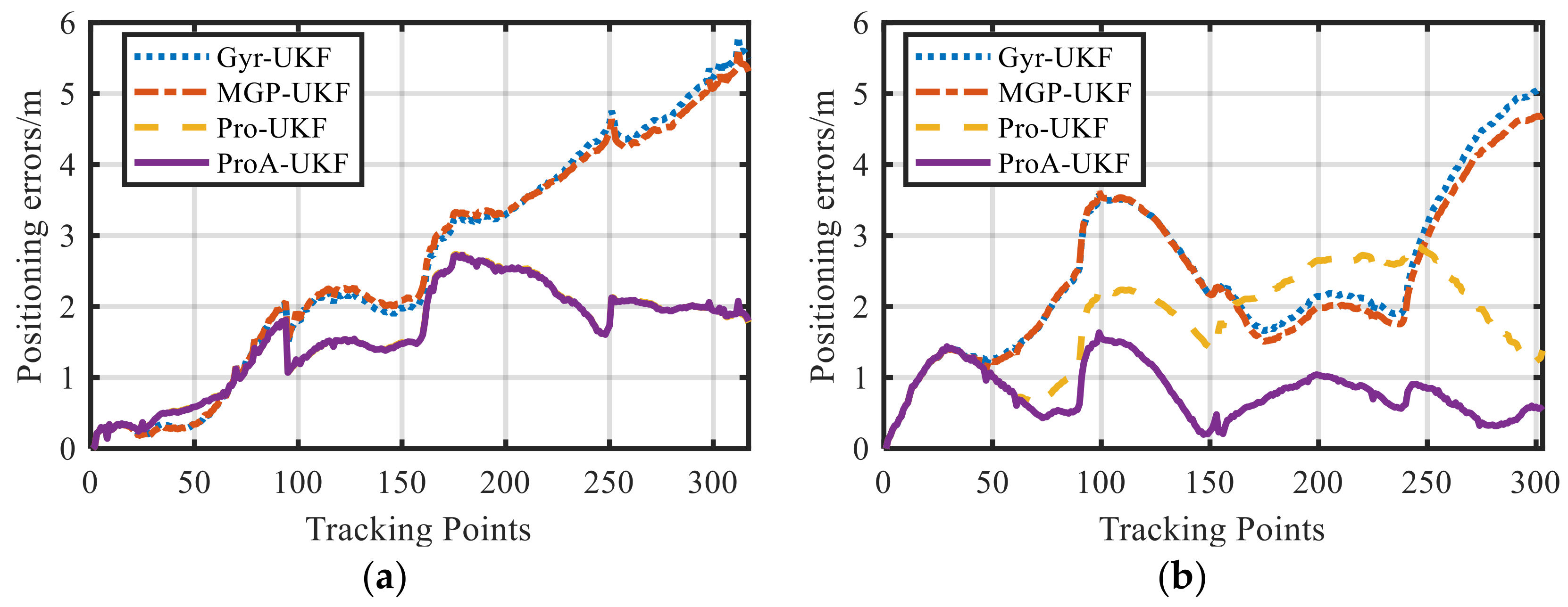
7.2. Kinematic Experiment

The kinematic data were used to further verify the effectiveness of the proposed algorithm. The site of data collection was on the third floor of the J9 office building of Shandong University of Science and Technology, and many iron materials were on site. The floor plan is shown in Figure 3. The tester held the HV9 and XM8 smartphones in their hand to collect data along the preplanned trajectory.

Figure 4 shows the calculated heading that used the data collected by the HV9 and XM8, and true north was used to largely avoid the heading jumps between 0 and 360. Five methods were used for heading estimation in these kinematic experiments. The first was Mag, the second was Gyr, the third was proposed in [22] that the current heading was determined by magnetometer, gyroscope and previous estimate (MGP), the fourth was Pro that is the proposed method in this paper without the adaptive filter, and the last was ProA that the adaptive filter is used in Pro. And the reference is the reference heading in Figure 4. Compared to the other four methods, the heading based on the magnetometer severely jumped for these smartphones, and the maximum jump achieved 30 degrees, although the heading calculated by magnetic field was close to the reference at some locations. Thus, it is not appropriate to obtain the heading just using the outputs of the magnetometer for pedestrian navigation in complex indoor environments.

Figure 5 shows the heading errors of the local trajectory marked in A, B, C, and D in Figure 4a, and Figure 6 shows the heading errors of the local trajectory of Figure 4b. The heading errors of Mag for HV9 and XM8 are not shown in Figure 5 and Figure 6 because these errors fluctuate widely. However, these statistical results, of heading errors of these five methods for HV9 and XM8, are all shown in

Table 1. The statistic of heading errors for HV9.

	Mag		Gyr		MGP		Pro		ProA
	RMS/°	Mean/°	RMS/°	Mean/°	RMS/°	Mean/°	RMS/°	Mean/°	RMS/°	Mean/°
A	8.28	−0.84	2.40	1.10	2.20	1.00	1.74	0.09	1.74	0.12
B	8.73	−4.32	1.39	0.53	1.17	0.55	1.09	0.49	1.09	0.47
C	9.61	−5.74	3.13	−2.50	3.01	−2.47	1.26	0.05	1.27	0.04
D	7.85	−0.40	2.59	−2.06	2.38	−1.98	1.55	0.43	1.55	0.42
Mean/°	8.62	−2.83	2.38	−0.73	2.19	−0.73	1.41	0.27	1.41	0.26

and

Table 2. The statistic of heading errors for XM8.

	Mag		Gyr		MGP		Pro		ProA
	RMS/°	Mean/°	RMS/°	Mean/°	RMS/°	Mean/°	RMS/°	Mean/°	RMS/°	Mean/°
A	3.55	−0.08	3.55	2.67	3.45	2.50	2.25	1.07	1.70	0.47
B	10.20	6.50	3.77	0.76	3.66	0.88	3.28	1.85	2.69	−0.36
C	14.76	−10.95	5.41	3.92	5.35	3.99	3.39	2.85	2.02	1.00
D	15.02	−13.00	5.57	−4.58	5.51	−4.58	2.58	2.24	2.19	1.76
Mean/°	10.88	−4.38	4.58	0.69	4.49	0.69	2.88	2.00	2.15	0.71

, respectively. In Table 1 and Table 2, the mean RMSs of heading error for Mag are 8.62° and 10.88° for HV9 and XM8, respectively, and these accuracies are not appropriate for pedestrian navigation. In Figure 5a, most heading errors of Pro and ProA are within 4°, and these heading errors are smaller than those of Gyr and MGP. In Figure 5b–d, these heading errors of Pro and ProA are within 2°, and these accuracies of heading estimation are better than those of Gyr and MGP. In Table 1, the RMS of MGP is slightly superior to that of Gyr, and the mean RMS decreases from 2.38° to 2.19°. The accuracy of Pro is better than that of MGP in every section. The RMS decreases from 2.20° to 1.74° in the local trajectory of mark A, the RMS drops from 1.17° to 1.09° in the local trajectory of mark B, the RMS reduces from 3.01° to 1.26° in the local trajectory of mark C, and the RMS decreased from 2.38° to 1.55° in the local trajectory of mark D. And the mean accuracy increased by 35.62%. In Table 1, the accuracy of Pro is basically the same as that of ProA. We also can see from these lists of Mean in Table 1 that these results of heading estimation are bias. The first reason for this bias is that the tester cannot strictly walk in accordance with the preplanned trajectory, and the other is that the smartphone will inevitably shake with the movement of the tester. These conditions can cause the biased estimation. We can see from Table 1, the bias of Pro and ProA is smaller than that of the other methods. In summary, compared with the heading estimated by Mag, Gyr and MGP, the heading solved by the proposed algorithm is close to the reference for this experiment.

Figure 6 shows local heading error of Figure 4b. In Figure 6a, most errors of Pro and ProA are within 4°, and these errors are smaller than those of Gyr and MGP. In Figure 6b–d, these errors of Pro and ProA are principally less than 5°, and these results of Pro and ProA are superior to those of Gyr and MGP. In Table 2, The RMS of MGP is slightly smaller than that of Gyr, and the mean RMS is decreased by 1.97%. For these two kinematic experiments, the accuracy of heading estimation for MGP is better than that of Gyr, and this conclusion is consistent with that of the literature [22]. We can also see from Table 2 that these accuracies of Pro are better than those of MGP in these four sections. The RMS decrease from 3.45° to 2.25° in the local trajectory of mark A, the RMS drops from 3.66° to 3.28° in the local trajectory of mark B, the RMS reduces from 5.35° to 3.39° in the local trajectory of mark C, and the RMS decreases from 5.51° to 2.58° in the local trajectory of mark D. Compared with the mean accuracy of MGP, the mean accuracy of Pro increases by 35.86%. In Table 2, the accuracy of heading estimation is further improved by the adaptive algorithm. The RMS decreases from 2.25° to 1.70° in the local trajectory of mark A, the RMS drops from 3.28° to 2.69° in the local trajectory of mark B, the RMS reduces from 3.39° to 2.02° in the local trajectory of mark C, and the RMS decreases from 2.58° to 2.19° in the local trajectory of mark D. Also, the mean of RMS is improved by 25.35% for this kinematic data. Similarly, the biased heading estimation can be observed in Table 2, and the bias of mean for ProA is the smallest among these methods. Compared with these methods of Mag, Gyr and MGP, these methods of Pro and ProA can obtain the higher accuracy of heading estimation.

In order to intuitively and precisely express the accuracy of heading estimation, the estimated heading was used for the positioning estimation of PDR. The method of Mag was not used to estimate the position in this section because the heading accuracy is poor, and we designed four programs to obtain the position estimation of these two kinematic experiments.

(1)

The Gyr is used to calculate heading, and UKF is used for position estimation (Gyr-UKF).

(2)

The MGP is used to obtain heading, and position is estimated based on UKF (MGP-UKF).

(3)

The Pro is applied to estimate heading, and position estimation is obtained by UKF (MGP-UKF).

(4)

The ProA is applied to estimate heading, and UKF is used for position estimation (MGP-UKF).

We compare the position estimation of these four methods in this section.

Figure 7 shows the position trajectories calculated by the outputs of the HV9. We can see from Figure 7 that these position trajectories of Gyr-UKF and MGP-UKF deviate from the reference with time, and the results of position estimation for these two methods are almost identical. The trajectory is improved by the method of Pro-UKF, and the position trajectory of ProA-UKF is basically the same as that of Pro-UKF. Figure 8 shows these trajectories obtained by XM8. We can see that these trajectories of Gyr-UKF and MGP-UKF deviate from the reference with time, and the trajectory of MGP-UKF is slighter better than that of Gyr-UKF. The trajectory is improved by the method of Pro-UKF, and the trajectory is further improved when ProA is used to estimate heading. Therefore, the trajectory calculated by a ProA-UKF algorithm is more accurate than that obtained by the other three methods.

In order to provide a reference at each step, these timestamps were recorded when the tester passed corners, and the coordinates of these corners can be obtained by the reference trajectory and reference heading. The coordinates of each step between these two corners can be calculated by linear interpolation in time. In order to accurately analyze the heading, the step-length error is ignored here. Figure 9 shows the 2D position error of each step using HV9 and XM8. Figure 9a shows the position error of HV9. When the method of Gyr-UKF and MGP-UKF is used, the position error gradually accumulates with the walking distance, and the maximum error exceeds 5.5 m. The estimated position of MGP-UKF is slightly better than that of Gyr-UKF. The position error is improved by the Pro-UKF, and the maximum error is less than 2.8 m. We can also see that the position error of ProA-UKF is slightly smaller than that of Pro-UKF. Figure 9b is the position error of XM8 for different methods. The position error deviates from the reference with time when the Gyr-UKF is used, and the maximum error is over 5.0 m. The position estimation is slightly improved when MGP-UKF is used. The position errors are effectively constrained when the proposed algorithm of Pro-UKF is used, and the maximum error is less than 3.0 m. The position errors are further improved if the adaptive algorithm is used to estimate the heading, and the maximum error is less than 2.0 m. In Figure 9b, the positions accuracy of Pro-UKF is worse than those of Gyr-UKF and MGP-UKF at times. We can see from Figure 6c that the heading error is mostly positive for Pro, that will make the error accumulate, and the heading errors have positive and negative values for Gyr and MGP that will offset the error accumulation.

The corresponding position cumulative error estimation percentages (CEF) of Figure 9 is explained in Figure 10. In Figure 10a, the CEF within 1.5 m is 24.92% and 25.24% for Gyr-UKF and MGP-UKF, respectively, and the CEF is raised to 40.38% and 41.01% for Pro-UKF and ProA-UKF, respectively. The CEF within 2 m are 38.80% and 31.86% for Gyr-UKF and MGP-UKF, respectively. The CEF is increased to 68.45% for both Pro-UKF and ProA-UKF. When the CEF is about 75%, the position error is over 4 m for Gyr-UKF and MGP-UKF, and the position error is less than 2.25 m for Pro-UKF and ProA-UKF. For HV9, the proposed method can enhance the accuracy of position estimation. Figure 10b shows the CEF of XM8. In Figure 10b, the CEF within 1.5 m is just 20.79% for both Gyr-UKF and MGP-UKF, the CEF achieves 36.30% for Pro-UKF, and the CEF is, as expected, increased to 97.03% for ProA-UKF. When the position error is within 2 m, the CEF is 38.94% and 47.52% for Gyr-UKF and MGP-UKF, respectively, and the CEF is slight improved for Pro-UKF with 50.50%, however, the CEF is raised to 100% when the ProA-UKF is used. When the CEF is about 75%, the position errors are both over 3.25 m for Gyr-UKF and MGP-UKF, the error is within 2.50 m for Pro-UKF, and the error is less than 1.25 m for ProA-UKF. Therefore, we can obtain the conclusion that the proposed algorithm can improves the accuracy of heading estimation for smartphone.

Table 3. Statistics of position error with different method for different smartphone.

		Gyr-UKF	MGP-UKF	Pro-UKF	ProA-UKF
HV9	Max/m	5.80	5.63	2.75	2.73
	Mean/m	2.67	2.65	1.60	1.59
	RMS/m	3.14	3.10	1.75	1.74
XM8	Max/m	5.05	4.69	2.89	1.63
	Mean/m	2.47	2.38	1.81	0.80
	RMS/m	2.73	2.62	1.94	0.87

shows the statistics of position errors. In Table 3, the mean errors of position estimation for PDR are 2.67 m, 2.65 m, 1.60 m and 1.59 m for these four respective schemes of position estimation, and the corresponding RMS values are 3.14 m, 3.10 m, 1.75 m and 1.74 m for the HV9 smartphone. For the XM8 smartphone, the mean errors are 2.47 m, 2.38 m, 1.81 m and 0.80 m, and the RMS values are 2.73 m, 2.62 m, 1.94 m and 0.87 m for these four respective schemes. The estimated position by ProA-UKF, where the adaptive filter is used to estimate heading, is better than that by Pro-UKF, the position error of Pro-UKF is smaller than that of the traditional method and the position error of MGP-UKF is slightly superior to that of Gyr-UKF. Compared with the method of MGP, the mean error of ProA-UKF is reduced by 40.00%, and RMS is improved by 43.87% for the HV9. And the mean error is reduced by 66.39%, and the RMS is improved by 66.79% for the XM8. Therefore, the method of heading estimation proposed in this paper can improve the accuracy of heading estimation, and it directly enhances the accuracy of position estimation for pedestrian navigation.

8. Conclusions

A novel method of heading estimation based on smartphones is proposed in this paper. This method uses the AR model to build KF, and the current heading—determined by fusing these headings calculated by magnetometer, estimated by gyroscope and stored by the previous estimate—is used as measurement value of KF update. To effectively suppress the accumulated error of the heading estimated by the outputs of the gyroscope, the estimated heading by KF in QS is used to correct the heading calculated by gyroscope. To improve the accuracy of heading estimation, an AKF based on the innovation sequence is used to adaptively adjust the state noise covariance. HV9 and XM8 smartphones were used to collect data. In order to intuitively and precisely express the accuracy of heading estimation, the estimated heading is also used for the position estimation of PDR. The following conclusions were obtained,

(1)

The heading calculated by a magnetometer is susceptible to disturbances in the complex indoor environment that can cause dozens of degrees bias. Also, it is possible that the heading calculated by magnetometer is close to the reference at some locations. The heading estimated by gyroscope is affected by cumulative error. The heading obtained by the proposed method can not only reduce the noise but also constraint the cumulative error.

(2)

Compared with the mean accuracy of traditional methods for heading estimation, the mean accuracy of the heading estimated by proposed algorithm is increased by 35.62% and 35.86%, respectively, for HV9 and XM8. And compared with KF, AKF can further improve the accuracy of heading estimation.

(3)

The estimated heading is used for position calculation of PDR. Compared to traditional methods, the mean errors of position estimation for the proposed method decrease by 40.00% and 66.39%, and the corresponding RMS is improved by 43.87% and 66.79%, respectively, for HV9 and XM8 smartphones with different performance sensors.

References

1. Alletto, S.; Cucchiara, R.; Fiore, G.; Mainetti, L.; Mighali, V.; Patrono, L.; Serra, G. An indoor location-aware system for an IoT-based smart museum. IEEE Internet Things J. 2016, 3, 244–253. [Google Scholar] [CrossRef]
2. Chen, J.; Ou, G.; Peng, A.; Zheng, L.; Shi, J. An INS/WiFi indoor localization system based on the weight least squares. Sensors 2018, 15, 1458. [Google Scholar] [CrossRef] [PubMed]
3. Liu, H.; Yang, J.; Sidhom, S.; Wang, Y.; Chen, Y.; Ye, F. Accurate WiFi based localization for smartphone using peer assistance. IEEE Trans. Mob. Comput. 2014, 13, 2199–2213. [Google Scholar] [CrossRef]
4. Li, X.; Wang, J.; Liu, C. A Bluetooth/PDR integration algorithm for an indoor positioning system. Sensors 2015, 15, 24862–24885. [Google Scholar] [CrossRef]
5. Chen, P.; Kuang, Y.; Chen, X. A UWB/Improved PDR Integration Algorithm Applied to Dynamic Indoor Positioning for Pedestrians. Sensors 2017, 17, 2065. [Google Scholar] [CrossRef]
6. Harle, R. A survey of indoor inertial positioning systems for pedestrians. IEEE Commun. Surv. Tutor. 2013, 15, 1281–1293. [Google Scholar] [CrossRef]
7. Li, X.; Wang, J.; Liu, C.; Zhang, L.; Li, Z. Integrated WiFi/PDR/Smartphone using an adaptive system noise extended Kalman filter algorithm for indoor localization. Int. J. Geo-Inf. 2016, 5, 8. [Google Scholar] [CrossRef]
8. Chen, R.; Chen, L. Indoor positioning with smartphones: The state-of-art and challenges. Acta Geod. Cartogr. Sin. 2017, 46, 1316–1326. [Google Scholar]
9. Li, Y.; Zhuang, Y.; Lan, H.; Zhou, Q.; Niu, X.; El-Sheimy, N. A hybrid WiFi/Magnetic matching/PDR approach for indoor navigation with smartphone sensors. IEEE Commun. Lett. 2016, 20, 169–172. [Google Scholar] [CrossRef]
10. Kuang, J.; Niu, X.J.; Chen, X. Robust pedestrian dead reckoning based on MEMS-IMU for smartphone. Sensors 2018, 18, 1391. [Google Scholar] [CrossRef] [PubMed]
11. Davidson, P.; Takala, J. Algorithm for pedestrian navigation combining IMU measurements and gait models. Gyroscope Navig. 2013, 4, 79–84. [Google Scholar] [CrossRef]
12. Gu, Y.; Song, Q.; Li, Y.; Ma, M. Foot-mounted pedestrian navigation based on particle filter with an adaptive weight updating strategy. J. Navig. 2015, 68, 23–38. [Google Scholar] [CrossRef]
13. Zhuang, Y.; Lan, H.; Li, Y.; El-Sheimy, N. PDR/INS/WiFi integration based on handheld devices for indoor pedestrian navigation. Sensors 2015, 6, 793–812. [Google Scholar] [CrossRef]
14. Kim, Y.; Choi, S.; Kim, H.; Lee, J. Performance improvement and height estimation of pedestrian dead-reckoning system using a low cost MEMS sensor. In Proceedings of the 12th International Conference on Control, Automation and Systems, Jeju Island, Korea, 17–21 October 2012. [Google Scholar]
15. Kang, W.; Nam, S.; Lee, S. Improved heading estimation for smartphone-based indoor positioning systems. In Proceedings of the 2012 IEEE 23rd International Symposium on Personal, Indoor and Mobile Radio Communications, Sydney, Australia, 9–12 September 2012. [Google Scholar]
16. Brajdic, A.; Harle, R. Walk detection and step counting on unconstrained smartphones. In Proceedings of the 2013 ACM International Joint Conference on Pervasive and Ubiquitous Computing, Zurich, Switzerland, 8–12 September 2013. [Google Scholar]
17. Hasan, M.; Mishuk, M. MEMS IMU based pedestrian indoor navigation for smart glass. Wirel. Pers. Commun. 2018, 101, 287–303. [Google Scholar] [CrossRef]
18. Tian, Z.; Zhang, Y.; Zhou, M.; Liu, Y. Pedestrian dead reckoning for MARG navigation using a smartphone. J. Adv. Signal Process. 2014, 65, 65–73. [Google Scholar] [CrossRef]
19. Gade, K. The seven ways to find heading. J. Navig. 2016, 69, 955–970. [Google Scholar] [CrossRef]
20. Afzal, M.; Renaudin, V.; Lachapelle, G. Magnetic field based heading estimation for pedestrian navigation environments. In Proceedings of the 2011 International Conference on Indoor Positioning and Indoor Navigation, Guimaraes, Portugal, 21–23 September 2011. [Google Scholar]
21. Zheng, Z.; Hu, Y.; Yu, J.; Na, Z. Extended Kalman filter for real time indoor localization by fusing WiFi and smartphone inertial sensors. Sensors 2015, 6, 523–543. [Google Scholar]
22. Kang, W.; Han, Y.N. SmartPDR: Smartpone-based pedestrian dead reckoning for indoor localization. IEEE Sens. J. 2015, 15, 2906–2916. [Google Scholar] [CrossRef]
23. Valenti, R.; Dryanovski, I.; Xiao, J. A linear Kalman filter for MARG orientation estimation using the algebraic quaternion algorithm. IEEE Trans. Instrum. Meas. 2015, 65, 467–481. [Google Scholar] [CrossRef]
24. Renaudin, V.; Combettes, C.; Peyret, F. Quaternion based heading estimation with handheld MEMS in indoor environments. In Proceedings of the IEEE/ION Positioning, Location and Navigation Symposium, Monterey, CA, USA, 5–8 May 2014. [Google Scholar]
25. Yuan, X.; Yu, S.; Zhang, S. Quaternion-based unscented Kalman filter for accurate indoor heading estimation using wearable multi-sensor system. Sensors 2015, 15, 10872–10890. [Google Scholar] [CrossRef]
26. Afzal, M.; Renaudin, V.; Lachapelle, G. Use of earth’s magnetic field for mitigating gyroscope errors regardless of magnetic perturbation. Sensors 2011, 11, 11390–11414. [Google Scholar] [CrossRef]
27. Ali, A.; El-Sheimy, N. Low-cost MEMS-based pedestrian navigation technique for GPS-denied areas. J. Sens. 2013, 2013, 197090. [Google Scholar] [CrossRef]
28. Mohamed, A.; Schwarz, K. Adaptive Kaman filtering for INS/GPS. J. Geod. 1999, 73, 193–203. [Google Scholar] [CrossRef]
29. Chang, G.; Liu, M. An adaptive fading Kalman filter based on Mahalanobis distance. Proc. Inst. Mech. Eng. Part G J. Aerosp. Eng. 2015, 229, 1114–1123. [Google Scholar] [CrossRef]
30. Jiang, C.; Zhang, S. A novel adaptively-robust strategy based on the Mahalanobis distance for GPS/INS integrated navigation systems. Sensors 2018, 18, 695. [Google Scholar] [CrossRef]
31. Wu, D.; Xia, L.; Geng, J. Heading estimation for pedestrian dead reckoning based on robust adaptive Kalman Filtering. Sensors 2018, 18, 1970. [Google Scholar] [CrossRef]
32. Li, W.; Wang, J. Effective adaptive Kalman filter for MEMS-IMU/Magnetometers integrated attitude and heading reference system. J. Navig. 2013, 66, 99–113. [Google Scholar] [CrossRef]
33. Jin, B.; Guo, J.; He, J.; Guo, W. Adaptive Kalman filter based on optimal autoregressive predictive model. GPS Solut. 2017, 21, 307–317. [Google Scholar] [CrossRef]
34. Jin, B.; Su, T.; Zhang, W.; Zhang, L. Joint optimization of predictive model and transmitted waveform for extended target tracking. In Proceedings of the 2014 12th International Conference on Signal Processing (ICSP), Hangzhou, China, 19–23 October 2014. [Google Scholar]
35. Ding, W.; Wang, J.; Rizos, C. Improving adaptive Kalman estimation in GPS/INS integration. J. Navig. 2007, 60, 517–529. [Google Scholar] [CrossRef]
36. Renaudin, V.; Afzal, M.; Lachapelle, G. Complete triaxis magnetometer calibration in the magnetic domain. J. Sens. 2010, 2010, 967245. [Google Scholar] [CrossRef]
37. Klingbeik, L.; Eling, C.; Zimmermann, F.; Kuhlmann, H. Magnetic field sensor calibration for attitude determination. J. Appl. Geod. 2014, 8, 97–108. [Google Scholar]
38. Ma, M.; Song, Q.; Gu, Y.; Zhou, Z. Use of magnetic field for mitigating gyroscope errors for indoor pedestrian positioning. Sensors 2018, 18, 2592. [Google Scholar] [CrossRef]
39. Li, F.; Zhao, C.; Ding, G.; Gong, J.; Liu, C.; Zhao, F. A reliable and accurate indoor location method using phone inertial sensors. In Proceedings of the 2012 ACM Conference on Ubiquitous Computing, New York, NY, USA, 5–8 September 2012. [Google Scholar]
40. Chen, G.; Meng, X.; Wang, Y.; Zhang, Y.; Tian, P.; Yang, H. Integrated WiFi/PDR/Smartphone using an unscented Kalman filter algorithm for 3D indoor localization. Sensors 2015, 15, 24595–24614. [Google Scholar] [CrossRef]
Figure 1. The body coordinate system of smartphone.
Applsci 09 03727 g001
Figure 2. Heading error of static data for different methods: (a) The heading error of Huawei Honor V9 (HV9); (b) The heading error of XiaoMi8 (XM8).
Applsci 09 03727 g002
Figure 3. Trajectory of experiment: (a) Floor plan; (b) Experimental environment.
Applsci 09 03727 g003
Figure 4. Heading estimation with different methods for different smartphones: (a) Heading of HV9; (b) Heading of XM8.
Applsci 09 03727 g004
Figure 5. Heading error of local trajectory for HV9: (a) Heading error of mark A; (b) Heading error of mark B; (c) Heading error of mark C; (d) Heading error of mark D.
Applsci 09 03727 g005
Figure 6. Heading error of local trajectory for XM8: (a) Heading error of mark A; (b) Heading error of mark B; (c) Heading error of mark C; (d) Heading error of mark D.
Applsci 09 03727 g006
Figure 7. Trajectories of different heading estimations for HV9.
Applsci 09 03727 g007
Figure 8. Trajectories of different heading estimations for XM8.
Applsci 09 03727 g008
Figure 9. Position error of each step with different methods for different smartphones: (a) The position error of HV9; (b) The position error of XM8.
Applsci 09 03727 g009
Figure 10. Position cumulative error percentages of different methods for different smartphones: (a) The error percentage for HV9; (b) The error percentage for XM8.
Applsci 09 03727 g010