Parallel Image Completion with Edge and Color Map

Abstract

Over the last few years, image completion has made significant progress due to the generative adversarial networks (GANs) that are able to synthesize photorealistic contents. However, one of the main obstacles faced by many existing methods is that they often create blurry textures or distorted structures that are inconsistent with surrounding regions. The main reason is the ineffectiveness of disentangling style latent space implicitly from images. To address this problem, we develop a novel image completion framework called PIC-EC: parallel image completion networks with edge and color maps, which explicitly provides image edge and color information as the prior knowledge for image completion. The PIC-EC framework consists of the parallel edge and color generators followed by an image completion network. Specifically, the parallel paths generate edge and color maps for the missing region at the same time, and then the image completion network fills the missing region with fine details using the generated edge and color information as the priors. The proposed method was evaluated over CelebA-HQ and Paris StreetView datasets. Experimental results demonstrate that PIC-EC achieves superior performance on challenging cases with complex compositions and outperforms existing methods on evaluations of realism and accuracy, both quantitatively and qualitatively.

1. Introduction

Image completion (a.k.a. image inpainting or image hole-filling) aims at synthesizing alternative structures and textures that visually realistic contents in the missing or damaged regions of an image. It is essential in many image editing tasks and has aroused wide interest in the computer vision and graphic community as it can be used for repairing damaged photographs or filling in holes left after removing the distracting objects from an image. It can also be extended to problems such as digital effect (e.g., object removal), image restoration (e.g., scratch or text removal in photograph), image coding and transmission (e.g., recovery of the missing blocks), rotation, stitching, retargeting, recomposition, super-resolution and many others. Therefore, the generated contents should either be as accurate as the original image, or simply fit well within the context such that the modification appears to be visually natural, photorealistic and semantically correct.

In general, image completion can be divided into two categories: generic scene image completion and specific image completion (e.g., human faces). Due to the well-known compositionality and reusability of visual patterns, missing regions in the former usually have a high chance of finding similar patterns in either the surrounding context of the same image or images in an external dataset subject to the context. However, the latter cases are more specific, especially when a large essential portion of an image is missing. The objective of image completion should be not only photorealistic but also semantically consistent with the surrounding image context at different scales. First, structural features should remain connected inside the missing region or across its boundary. Second, colorization should be plausible and spatially coherent that could potentially fool a human observer. Third, textures filled within the missing region should contain high-frequency details. In addition, missing object parts need to be recovered correctly, which is challenging and requires capturing high-level semantics.

The core challenge of image completion problems lies in the inherent ambiguity of this ill-posed inverse problem and synthesizing content with reasonable details for the missing regions that are often not coherent with the surrounding areas. The main reason is that modeling the pixel distribution is difficult and the trained models easily introduce blurry components and artifacts when the dimensionality becomes very high. Therefore, sufficient prior information is required to achieve meaningful and visually believable results.

There have been a number of studies attempting to solve this problem. These studies fall into two groups: data similarity driven methods with low-level features and data distribution based generative ones. Broadly speaking, methods in the first group can be classified into two categories: diffusion-based methods [1,2,3,4,5] and patch-based methods [6,7,8,9,10,11,12,13,14]. Diffusion-based methods solve Partial Differential Equations (PDE) [1] or similar diffusion systems, so as to diffuse the information from the known region into the missing region at the pixel level. They have achieved convincingly excellent results for filling narrow or small holes. However, they tend to introduce smooth effects in the textured region or larger missing region. Patch-based methods are capable of recovering large missing regions by copying suitable textures in the known contexts and then pasting them into the missing region from low-resolution to high-resolution at patch level. They can synthesize plausible stationary textures and perform particularly well in background completion tasks (e.g., grass, sky and mountain), and are widely deployed in practical applications [11]. However, this copy and paste strategy assumes that the missing patches can be found somewhere in the same image; it cannot hallucinate novel image contents for challenging cases where the missing region involves complex and non-repetitive structures (e.g., multiple textures meeting at the border of the missing region). Moreover, although such methods are good at propagating high-frequency texture details, they are not able to capture high-level semantics or global structures of the missing region. Furthermore, matching patch is a computationally expensive operation. An alternative is the data-driven method [15], which retrieves plausible patches from a large database based on context similarity to repair a damaged image. This method assumes that the regions surrounded by similar context likely posses similar content. It is very effective when it finds an example image with sufficient visual similarity to the query and is often utilized for generic scene completion. However, it is bound to fail when no similar exemplars can be found in either the context or the external database. This limitation greatly restricts its possible application scenarios.

Not only is it necessary to complete textured patterns, it is also important to understand the anatomy of the scenes and objects being completed. Instead of seeking similar patches, the methods in the second group learn the underlying distribution governing the data generation with respect to the context. More recently, much progress has been made [16,17,18,19,20,21,22,23] in this direction due to the resurgence of deep learning [24], especially the generative adversarial networks (GANs) [25]. In this paradigm, image completion has been formulated as a conditional image generation problem and solved with GANs which introduce the concept of adversarial learning between a generator and a discriminator. These learning-based methods are able to hallucinate novel contents in the missing region by training on a large scale dataset.

However, most of the learning-based methods assume that the generative models can implicitly predict or understand the structure and semantic priors in the image, without explicitly modeling them in the learning process. Unfortunately, this strategy often struggles to reconstruct high frequency details in the generated regions accurately. This is mainly because the distribution of natural images is very complex and it is difficult to model this distribution directly at the pixel level. Thus, neither structural continuity nor texture consistency can be guaranteed between the missing region and the remaining image context. How, then, should we guide an image completion method generating coherent structures and fine details in the missing region?

Inspired by the image-to-image translation [26,27], we propose an universal image completion framework called PIC-EC: parallel image completion networks with edge and color priors, which explicitly provides image edge and color maps as the prior knowledge for image completion. PIC-EC decouples the image completion problem into three relatively easy sub-problems that can be modeled using the GANs. The edge and color maps should be restored firstly because they have also been lost in the missing region. Edge and color maps recovery is a relatively easier task than image completion. Secondly, the restored edge and color maps can be used as the priors for the following image completion. Therefore, PIC-EC is a two-stage model that can be summarized into three parts: edge map recovery, color map recovery and fine details completion. During the first two parts, edge and color generators provide basic structure and elements information. In the last part, the missing regions are gradually refined with fine details, laying on increasingly intense layers of color, which add lights and shadow.

The proposed method is evaluated on two standard datasets CelebA-HQ [28] and Paris StreetView [29]. We compare the performance of our method against current state-of-the-art methods in terms of qualitative and quantitative. This paper makes the following contributions:

• The image completion problem is decoupled into three sub-problems that can be modeled using the GANs.
• A novel image completion framework named PIC-EC that combines edge and color maps to fill in the missing regions exhibiting fine details.
• Edge and color generators capable of hallucinating sparse edge and flat color maps in the missing regions given the surrounding context.
• An end-to-end trainable network that combines edge and color generation with image completion to generate fine details in missing regions.

The remaining parts of this paper proceeds as follows. Relevant research background is introduced in Section 2. Section 3 presents the details of the proposed PIC-EC method. Experiments are carried out and analyzed in Section 4 to demonstrate the effectiveness of the PIC-EC method. Section 5 reviews and discusses experimental results, and, in Section 6, we conclude the paper with a summary of key points.

2. Related Works

A variety of different methods have been proposed for the image completion task. These methods can be roughly divided into two mainstreams: traditional methods based on pixel propagation or patch matching, and recent methods based on deep neural networks. The first mainstream includes diffusion-based [1,2,3,4,5] and patch-based methods [6,7,11]. Diffusion-based methods synthesize textures by propagating the neighborhood region appearance to the missing region and are well founded on the PDE [1] theory and quite effective for small or narrow holes such as scratches found commonly in old photographs. However, they tend to introduce significant visual artifacts in the textured region and fail to recover meaningful contents in larger missing regions due to the lack of semantic texture or structure synthesis.

In contrast to the diffusion-based methods, patch-based ones fill in the missing regions by searching and copying information from the similar regions of the same image or a collection of images. They result in a better performance in handling more complicated cases that fill larger holes in the natural images. This idea stems from the texture synthesis technique [6], in which the missing region is filled by searching for the most similar and relevant patches from the uncorrupted regions. However, natural images are composed of structures and textures, in which the structures constitute the primal sketches of an image and the textures are image regions with homogenous patterns. Texture synthesis methods cannot handle the missing region with composite structures and textures. In order to find suitable image patches, bidirectional similarity [30] is proposed to capture more visual information and introduces less visual artifacts when calculating the patch similarity. Bertalmio et al. [4] propose to decompose the image into structure and texture layers, then complete the structure layer using diffusion-based methods and texture layer using the texture synthesis technique. It overcomes the smooth effect in the diffusion-based methods, but it’s still hard to recover the structure of the larger missing region. Criminisi et al. [7] and Telea et al. [31] design the patch-based methods by propagating the known patches into the missing patches gradually. However, these methods are computationally expensive since they work in an iterative way. To reduce the runtime and improve memory efficiency, tree-structure based search [32] and randomized method [11] are proposed. PatchMatch [11] is a typical patch-based method that has shown notable results for image editing applications including image completion. It is implemented as the Content Aware Fill in Adobe Photoshop and arguably among the current state-of-the-arts in terms of both visual quality and speed. The major drawback of PatchMatch is that it searches for relevant patches from the whole image, without using any high level information to guide the search. Furthermore, it is unable to generate novel objects not found in the source image. These patch-based methods assume that the known regions have similar semantic contents with the missing regions, which may not be true in some scenarios such as face image completion. Therefore, they may work well in some images with repetitive structures but cannot generate reasonable results for images with unique structures.

To generate semantically new content, Hays and Efros [15] proposed an image completion method using a large image database. This data-driven fashion method assumes that regions surrounded by similar context likely posses similar content. To complete a scene, images of the same scenes are retrieved from the database. By cutting the corresponding regions from the matched images and pasting them into the holes, the corrupted images can be repaired. However, this requires a high contextual match, which limits the applications greatly compared to the general approaches.

The second mainstream is the learning-based methods that employ deep neural networks to generate structures for the missing regions. These methods typically train a deep neural network as a mapping function from a corrupted image to a completed one in an end-to-end manner and have exhibited promising performance. A significant advantage of these methods over the non-learning ones is their ability to learn and understand adaptive image features of different semantics, which is especially important in cases of complex natural scenes, faces, objects and many others. The first learning-based method designed for image completion problem is context encoder (CE) [16], which uses an encoder–decoder architecture. The encoder maps a corrupted image to a low-dimensional feature space, which the decoder uses to construct the completed image. It trains a convolutional neural network to complete the center region of $64\times 64$ in a $128\times 128$ image, with an ${\ell }_2$ pixel-wise reconstruction loss in combination with a generative adversarial loss as the objective function. However, CE is only able to fill square holes at the center of an image, struggles to maintain global consistency and often generates results with visual artifacts. Yang et al. [17] initializes the hole with the output of CE and then propagates the high-frequency textures from the boundary to the missing area. This method requires solving a multi-scale optimization problem iteratively, which noticeably increases computational cost during inference. Furthermore, Iizuka et al. [19] extend CE by introducing both global and local discriminators to pay more attention on the missing regions. However, this method relies heavily on the post-processing of the completed image that blends both results from neural networks and traditional patch-based methods. Li et al. [20] introduce additional face parsing loss for face completion. In order to handle the irregular holes, Liu et al. [33] propose partial convolution for image completion, which uses masking and re-normalization steps to make the prediction of the missing pixels, is only conditioned on the valid positions in the feature maps. In the follow up study, Yu et al. [34] introduce gated convolution layer that learns the features of the masked region and presents masks automatically from data. These effectively prevent the convolution weights from capturing too many zeros when they traverse over the incomplete region.

Several methods have been proposed by providing additional information for image completion. Yeh et al. [21] search for the closest encoding in the latent space of the corrupted image and decode to get the completed image. However, this method is slow because back-propagation must be performed for every image during inference. Dolhansky and Ferrer [35] show the importance of exemplar information for image completion. This method is able to generate both sharp and realistic results. However, it is highly specialized and does not generalize well. Contextual attention module (CAM) [36] is proposed to model long-range spatial dependencies in images and integrated into networks to explicitly borrow information from distant spatial locations. It is a two-step approach to the image completion problem. In the first stage, it produces a coarse estimate of the missing region. Next, a refinement network sharpens the result using an attention mechanism by searching for a collection of background patches with the highest similarity to the coarse estimate. Nazeri et al. [23] introduce edge recovery as the prior for the image completion task. This method essentially decouples the recovery of high and low frequency information of the completed region. Yi et al. [37] propose the GMCNN (Generative Multi-column Convolutional Neural Networks) model to synthesize different image components in a parallel manner within one stage. Xin et al. [38] use a fusion block to generate a flexible alpha composition map providing a smooth fusion and an attention map to make the network focus more on the unknown regions.

3. Materials and Methods

3.1. Image Completion Problem Formulation

Given a corrupted image I with the missing region $\Omega$ and the remaining image context $\overline{\Omega }$, i.e., $I=\Omega \cup \overline{\Omega }$, the goal of image completion is to fill in the missing region $\Omega$ with realistic and appealing contents making use of the information in the known region $\overline{\Omega }$. The intensity of a pixel within the image I is denoted as $I(x,y)$, where $(x,y)$ is the coordinate of the pixel. M is a binary mask with $M(x,y)=1$ representing a missing pixel, given by:

$$M(x,y)=\left\{\begin{array}{cc}1,\hfill & \mathrm{if}(x,y)\in \Omega ,\hfill \\ 0,\hfill & \mathrm{if}(x,y)\in \overline{\Omega }.\hfill \end{array}\right.$$

(1)

Image completion task refers to a class of the linear inverse problems that tend to be ill-posed since there are an infinite number of feasible solutions, but only a few of them are natural images. A common approach for resolving this issue is to obtain a solution of the constrained optimization problem below:

$$I_{comp}^{*}=arg\underset{I_{comp}\in {\mathbb{I}}_{comp}}{min}{\mathbb{E}}_{\genfrac{}{}{0pt}{}{I\sim \mathbb{I}}{I_{gt}\sim {\mathbb{I}}_{gt}}}\left[D(F\left(I\right),I_{gt})\right],s.t.I=(1-M)\odot I_{gt},$$

(2)

where $\mathbb{I}$, ${\mathbb{I}}_{comp}$ and ${\mathbb{I}}_{gt}$ are the distributions of the corrupted images, the completed images and the ground truth images, $F:\mathbb{I}\mapsto {\mathbb{I}}_{comp}$ is a mapping function from the corrupted images to the completed images, $D(·)$ is the distance between the completed image and the ground truth image, and ⊙ denotes the Hadamard product.

Because of the complexity of the natural images, it is difficult to directly solve this linear inverse problem using the deep neural networks without any priors. The image priors serve as the regularizations that stabilize the degradation inversion, and direct the outcomes toward the more plausible results. In the image-to-image (I2I) translation field, some methods [26,27,39] disentangle the image in order to extract content and style respectively and can synthesize photorealistic images from the binary edge maps. Consequently, edge map is chosen as the structure prior to guide the image completion network generating semantic image contents with a more intact structure in the missing region. Color information also plays a critical role in the image-to-image translation. Compared with hand-designed priors, the edge and color maps can be learned directly from the image dataset. Therefore, they are tailored to the statistics of images in the dataset, and, in principle, provide stronger regularization to this inverse problem. Because the edge and color information have also been lost in the missing region, they should be restored firstly. The edge prior can be obtained from the constrained optimization problem below:

$$B_{comp}^{*}=arg\underset{B_{comp}\in {\mathbb{B}}_{comp}}{min}{\mathbb{E}}_{\genfrac{}{}{0pt}{}{B\sim \mathbb{B}}{B_{gt}\sim {\mathbb{B}}_{gt}}}\left[D_1(G_1\left(B\right),B_{gt})\right],s.t.B=(1-M)\odot B_{gt},$$

(3)

where $\mathbb{B}$, ${\mathbb{B}}_{comp}$ and ${\mathbb{B}}_{gt}$ are the distributions of the corrupted edge maps, the completed edge maps and the ground truth edge maps, $G_1:\mathbb{B}\mapsto {\mathbb{B}}_{comp}$ is a mapping function from the corrupted edge maps to the completed edge maps, and $D_1(·)$ is the distance between the completed edge map and the ground truth edge map.

The color prior can be obtained from the constrained optimization problem below:

$$C_{comp}^{*}=arg\underset{C_{comp}\in {\mathbb{C}}_{comp}}{min}{\mathbb{E}}_{\genfrac{}{}{0pt}{}{C\sim \mathbb{C}}{C_{gt}\sim {\mathbb{C}}_{gt}}}\left[D_2(G_2\left(C\right),C_{gt})\right],s.t.C=(1-M)\odot C_{gt},$$

(4)

where $\mathbb{C}$, ${\mathbb{C}}_{comp}$ and ${\mathbb{C}}_{gt}$ are the distributions of the corrupted color maps, the completed color maps and the ground truth color maps, $G_2:\mathbb{C}\mapsto {\mathbb{C}}_{comp}$ is a mapping function from the corrupted color maps to the completed color maps, $D_2(·)$ is the distance between the completed color map and the ground truth color map.

Therefore, the image completion problem can be formulated as:

$$I_{comp}^{*}=arg\underset{I_{comp}\in {\mathbb{I}}_{comp}}{min}{\mathbb{E}}_{\genfrac{}{}{0pt}{}{I\sim \mathbb{I}}{I_{gt}\sim {\mathbb{I}}_{gt}}}\left[D_3(G_3(I,B_{comp}^{*},C_{comp}^{*}),I_{gt})\right],s.t.I=(1-M)\odot I_{gt},$$

(5)

where $G_3:(\mathbb{I};{\mathbb{B}}_{comp},{\mathbb{C}}_{comp})\mapsto {\mathbb{I}}_{comp}$ is the mapping function from the corrupted images to the completed images with the edge and color priors, and $D_3(·)$ is the distance between the completed image and the ground truth image.

Thus, the image completion problem can be decoupled into three relatively easy sub-problems that can be modeled using the GANs. The mapping functions of $G_1$, $G_2$ and $G_3$ can be constructed as the generators and the distance measurements of $D_1$, $D_2$ and $D_3$ can be constructed as the discriminators in the GANs. The edge and color priors are learned from massive amounts of training data firstly, and then guide the following up image completion network to generate more realistic results. Inspired by this procedure, we design PIC-EC framework. As the name suggests, the parallel edge and color map networks are responsible for the edge and color map generation, respectively. In addition, the image completion network can convert these edge and color semantic information to a photorealistic image.

3.2. Architecture of PIC-EC

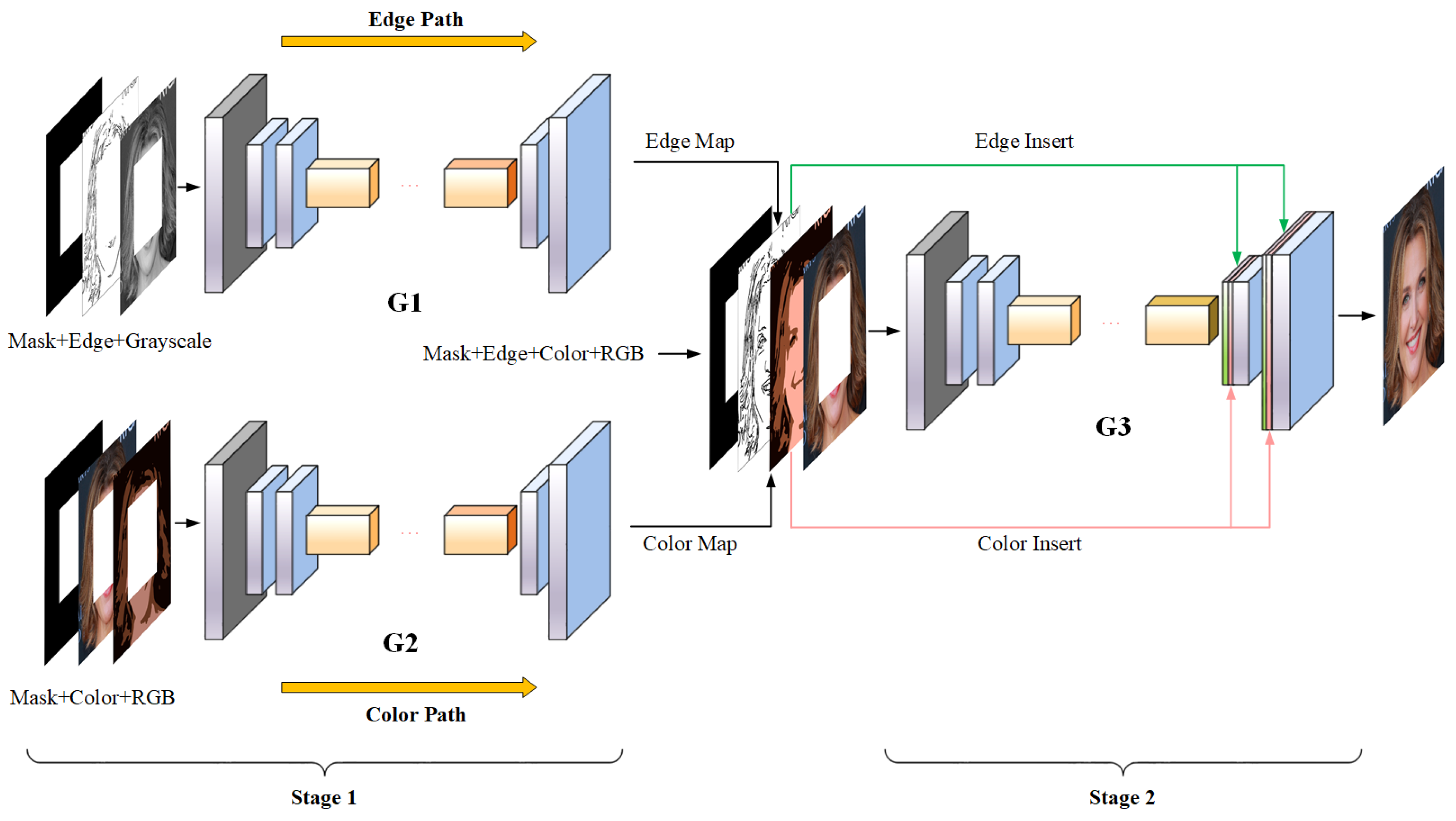
As shown in Figure 1, PIC-EC framework comprises of two stages: (1) the parallel edge and color map generators, and (2) the image completion network. The models in each stage follow the adversarial learning type, i.e., each model includes a generator/discriminator pair, and the discriminators are not shown for simplicity. $G_1$ and $D_1$ are the generator and discriminator for the edge path, $G_2$ and $D_2$ are the generator and discriminator for the color path, and $G_3$ and $D_3$ are the generator and discriminator for the image completion network, respectively. To simplify notation, these symbols are also used to represent the function mappings of their respective networks.

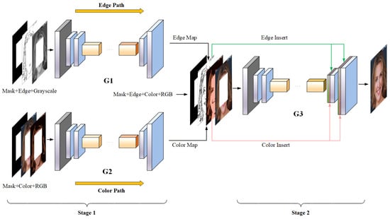
Figure 1. Overview of the PIC-EC (Parallel Image Completion with Edge and Color) framework for image completion. Masked edge map ${\tilde{E}}_{gt}$, masked grayscale image ${\tilde{I}}_{gray}$ and the mask M are the inputs of $G_1$ to predict the full edge map $E_{comp}$. Masked color map ${\tilde{C}}_{gt}$, masked RGB image ${\tilde{I}}_{gt}$ and the mask M are the inputs of $G_2$ to generate the full color map $C_{comp}$. Generated edge map, generated color map and masked RGB image are then concatenated with the mask, and fed to $G_3$ to get the completed image $I_{comp}$.

3.2.1. Generators

The generators in PIC-EC follow an encoder–decoder architecture similar to the network proposed by Johnson et al. [40], which has achieved impressive results for super-resolution, style transfer and image-to-image translation problems. This architecture allows for reducing the memory usage and computational time by initially decreasing the resolution before further processing the image. Specifically, the generator consists of encoders that down-sample twice, followed by eight residual blocks and decoders that up-sample images back to the same resolution as the input. The residual blocks make it easy for the network to learn the identify function. It is an appealing property for image completion task, since the output image should share structure with the input image. As listed in Table 1, the encoder includes one $7\times 7$ convolutional layer with stride 1 and 3 pixels reflection padding and two $4\times 4$ convolutional layers with stride 2 and 1 pixel reflection padding to reduce the spatial size by half while doubling the number of feature map channels. The reduced spatial dimensions allow convolution kernels to have a larger receptive field in the input image. The dilated convolution is used in the first layer of each residual block with dilation factor of 2. By employing dilated convolution, the generators can effectively enlarge the receptive field without increasing the amount of parameters and computational power. It plays an important role in the image completion task, as the context is critical for realism. The configuration of the generator is designed mainly according to the receptive field. We hope the receptive field of each neuron in the last layer can be as large as the input image size of $256\times 256$. This means that the neurons in the last layer can see the entire input image and more information can be used to generate contents. It is essential for the image completion problem. The receptive field of the configuration listed in Table 1 is $248\times 248$; it is very close to the input image size. In this case, the receptive field of neurons inside the generators is relatively large. In general, the kernel size corresponding to the large feature maps should be larger because the features in these feature maps tend to be larger. Therefore, the generator is designed to fulfill these conditions.

Table 1. Detailed architecture of the generators. After each convolutional layer, except the last one, there is a ReLU activation function. For $G_1$, the output layer channel is 1, and for $G_2$ and $G_3$, the output layer channel is 3.

Type	Kernel	Dilation	Stride	Channels
Convolution	$7\times 7$	1	$1\times 1$	64
Convolution	$4\times 4$	1	$2\times 2$	128
Convolution	$4\times 4$	1	$2\times 2$	256
ResBlock $\times 8$	$3\times 3$	2	$1\times 1$	256
Upsample ($\times 2\uparrow$)	-	-	-	256
Convolution	$3\times 3$	1	$1\times 1$	128
Upsample ($\times 2\uparrow$)	-	-	-	128
Convolution	$3\times 3$	1	$1\times 1$	64
Convolution	$7\times 7$	1	$1\times 1$	1 or 3

In order to avoid the notorious checkerboard artifact problem, the deconvolution layers in decoders were replaced with nearest neighbor interpolation upsampling layer and convolutional layer, and the two types of layer alternated. In the image completion generator $G_3$, the upsampling layers also concatenated with the edge and color information generated by $G_1$ and $G_2$, as shown in Figure 1. It can be seen as edge and color map insertion that effectively propagates the prior information throughout the image completion generator $G_3$ to make the image completion results more realistic and accurate. It should be noted that the edge and color maps should be resized to the same size as the corresponding layers in the decoders before concatenating with them.

After each convolutional layer, except the last one, there is a ReLU function. The final layer varies depending on the generator. In the generator $G_1$ and $G_2$, this layer has the channel size of 1 and 3 with sigmoid function, respectively. In the image completion generator $G_3$, the final layer has channel size of 3 with a tanh function for the prediction of an RGB image with the same size as the input. The spectral normalization (SN) [41] and instance normalization (IN) [42] are used across all layers of these generators. Although SN was originally proposed to be used only on the discriminator, previous works [43,44] have suggested that generators can also benefit from SN by suppressing sudden changes of parameter and gradient values.

3.2.2. Discriminators

The discriminators $D_1$, $D_2$ and $D_3$ in PIC-EC followed the $70\times 70$ SN-PatchGAN [34] architecture with SN, which allows a larger receptive field to detect the fake images. SN-PatchGAN applied GAN loss for each point in the output feature maps and effectively modelled the image as a Markov random field, assuming independence between pixels separated by more than a patch diameter. It was fast and stable during training and produced high-quality completion results. As listed in Table 2, the discriminators consist of five $4\times 4$ convolutional layers with 1 pixel zero padding. The first three layers have the stride of 2 and the rest are 1. LeakyReLU with slope 0.2 was employed after each layer except for the last one, which used a sigmoid function for the scores indicating whether each $70\times 70$ overlapping image patch is real or fake. Therefore, the receptive field of each neuron in the last layer is $70\times 70$, which can still cover the entire input image. In order to reduce the computational power and maintain the receptive field, $4\times 4$ is minimum kernel size meeting this requirement. The configuration listed in Table 2 is a reasonable choice. IN was also used across all layers of these discriminators.

Table 2. Detailed architecture of the discriminators. The output layer produces a score map instead of a single score, so as to tell the realism of different local regions of the input images.

Type	Kernel	Dilation	Stride	Channels
Convolution	$4\times 4$	1	$2\times 2$	64
Convolution	$4\times 4$	1	$2\times 2$	128
Convolution	$4\times 4$	1	$2\times 2$	256
Convolution	$4\times 4$	1	$1\times 1$	512
Convolution	$4\times 4$	1	$1\times 1$	1

3.3. Loss Function

Let $I_{gt}$ be the ground truth RGB image, and its edge map and color map counterparts will be denoted by $E_{gt}$ and $C_{gt}$, respectively. $I_{gray}$ is the corresponding grayscale image. In this paper, we composite the synthesized region and its known context together as a whole, and measure the loss between this composite image and the corresponding ground truth image.

3.3.1. Edge Path

The edge path was designed for solving the constrained optimization problem in Equation (3) to obtain the edge prior. For clarity, the letter E was used to represent the edge map. The input of edge generator $G_1$ was the masked edge map ${\tilde{E}}_{gt}=E_{gt}\odot (1-M)$ conditioned with its masked grayscale image ${\tilde{I}}_{gray}=I_{gray}\odot (1-M)$ and the mask M (1 for the missing region, 0 for background), illustrated in Figure 1. The edge map was predicted as:

$$E_{pred}=G_1\left({\tilde{E}}_{gt},{\tilde{I}}_{gray},M\right).$$

(6)

The composite edge map $E_{comp}$ was constructed by combining the background region of ground truth edge map $E_{gt}$ with the generated edge map $E_{pred}$ in the missing region:

$$E_{comp}=E_{gt}\odot (1-M)+E_{pred}\odot M.$$

(7)

Then, $E_{gt}$ and $E_{comp}$ are fed to the discriminator $D_1$ for adversarial training. If the input of $D_1$ is only the edge map ($E_{gt}$ or $E_{comp}$), the adversarial loss is hard to optimize and the training tends to fail. This is due to the sparse property of the edge map. Unlike the natural images that have an understandable distribution on each local region, the pixels in the edge map are sparsely distributed and contain less information for the discriminator to judge whether the generated distribution is close to the real distribution or not.

To address this problem, the edge maps $E_{gt}$ and $E_{comp}$ conditioned on $I_{gray}$ were adopted as the inputs of discriminator $D_1$. With this setup, the composite edge map $E_{comp}$ is not only required to be similar to the ground truth edge map $E_{gt}$, but also required to align with the edge information of the ground truth grayscale $I_{gray}$. The discriminator then obtained adequate knowledge to tell the difference between the fake distribution and the real distribution, and the training process became stable.

The network was trained with a joint loss that contained a feature matching loss ${\mathcal{L}}_{fm,1}$, a content loss ${\mathcal{L}}_{con}$, and an adversarial loss ${\mathcal{L}}_{adv}^{G_1}$, and the overall loss was computed below:

$${\mathcal{L}}_{G_1}={\lambda }_{fm,1}{\mathcal{L}}_{fm,1}+{\lambda }_{con}{\mathcal{L}}_{con}+{\lambda }_{adv,1}{\mathcal{L}}_{adv}^{G_1},$$

(8)

$${\mathcal{L}}_{D_1}={\mathcal{L}}_{adv}^{D_1},$$

(9)

where ${\lambda }_{fm,1}$, ${\lambda }_{con}$ and ${\lambda }_{adv,1}$ were the regularization parameters.

The feature matching loss ${\mathcal{L}}_{fm,1}$ compared the feature maps in the intermediate layers of the discriminator for the real and fake inputs. It stabilized the training process by forcing the generator to produce edge maps with representations that were similar to real ones. This is similar to the perceptual loss [40] where the feature maps are compared with those from the pre-trained VGG (Visual Geometry Group) network. However, since the VGG network was not trained on the edge dataset, it failed to capture the features that were in the edge model. The feature matching loss ${\mathcal{L}}_{fm,1}$ was defined as:

$${\mathcal{L}}_{fm,1}=\mathbb{E}\left[\sum _{i=1}^L\frac{1}{N_i}{∥D_1^{\left(i\right)}(E_{gt},I_{gray})-D_1^{\left(i\right)}(E_{comp},I_{gray})∥}_1\right],$$

(10)

where L is the number of layers in the discriminator $D_1$, $N_i$ is the number of elements in the ith layer and $D_1^{\left(i\right)}$ is the activations in the ith layer. Spectral normalization was introduced further to stabilize training process by scaling down weight matrices by their respective largest singular values, effectively restricting the Lipschitz constant of the network to one.

Due to the sigmoid activation function, each pixel in the edge map generated by $G_1$ can be interpreted as the probability that this pixel in the original image boundary. Hence, we can calculate the distance with the ground truth edge by computing their binary cross entropy between each location. Focal loss [45] was used to balance the importance of each pixel. Since the primary goal was to complete the missing edge map, the pixels in the missing region were provided a larger weight. Therefore, the content loss could be formulated as:

$${\mathcal{L}}_{con}=5M{(E_{pred}-E_{gt})}^2·{\mathcal{L}}_e^{\Omega }(E_{pred},E_{gt})+(1-M){(E_{pred}-E_{gt})}^2·{\mathcal{L}}_e^{\overline{\Omega }}(E_{pred},E_{gt}),$$

(11)

where M is the binary mask, ${\mathcal{L}}_e^{\Omega }$ and ${\mathcal{L}}_e^{\overline{\Omega }}$ are two cross entropy functions of the missing region and the remaining context region, respectively. The reason why the cross entropy was not replaced by the ${\ell }_1$ or ${\ell }_2$ distance is that they were not effective as the edge map was sparse, leading to the data imbalance problem.

In order to create a stable generator, LSGAN [46] was chosen to fit the real distribution with high frequency details. The adversarial losses for training the generator $G_1$ and the discriminator $D_1$ were expressed as follows, respectively:

$${\mathcal{L}}_{adv}^{G_1}=\frac{1}{2}\mathbb{E}\left[{\left(D_1(E_{comp},I_{gray})-1\right)}^2\right],$$

(12)

$${\mathcal{L}}_{adv}^{D_1}=\frac{1}{2}\mathbb{E}\left[{\left(D_1(E_{gt},I_{gray})-1\right)}^2\right]+\frac{1}{2}\mathbb{E}\left[D_1{\left(E_{comp},I_{gray}\right)}^2\right].$$

(13)

3.3.2. Color Path

The color path was designed for solving the constrained optimization problem in Equation (4) to obtain the color prior. The color generator $G_2$ used the masked color map ${\tilde{C}}_{gt}=C_{gt}\odot (1-M)$ as input, conditioned with masked RGB images ${\tilde{I}}_{gt}=I_{gt}\odot (1-M)$ and the mask M. Hence, the color map generated by $G_2$ was shown as:

$$C_{pred}=G_2\left({\tilde{C}}_{gt},{\tilde{I}}_{gt},M\right).$$

(14)

The composite color map $C_{comp}$ was obtained by combining the known region of ground truth color map $C_{gt}$ with the generated color map $C_{pred}$ in the missing region:

$$C_{comp}=C_{gt}\odot (1-M)+C_{pred}\odot M.$$

(15)

The discriminator $D_2$ took $C_{gt}$ and $C_{comp}$ as inputs to predict whether or not a patch of these color maps is real. The overall loss consisted of a feature matching loss ${\mathcal{L}}_{fm,2}$, a pixel-wise loss ${\mathcal{L}}_{pix,2}$ and an adversarial loss ${\mathcal{L}}_{adv}^{G_2}$; this can be formulated as follows:

$${\mathcal{L}}_{G_2}={\lambda }_{fm,2}{\mathcal{L}}_{fm,2}+{\lambda }_{pix,2}{\mathcal{L}}_{pix,2}+{\lambda }_{adv,2}{\mathcal{L}}_{adv}^{G_2},$$

(16)

$${\mathcal{L}}_{D_2}={\mathcal{L}}_{adv}^{D_2},$$

(17)

where ${\lambda }_{fm,2}$, ${\lambda }_{pix,2}$ and ${\lambda }_{adv,2}$ are the regularization parameters.

The feature matching loss ${\mathcal{L}}_{fm,2}$ in the color generator $G_2$ was similar to ${\mathcal{L}}_{fm,1}$. Because $C_{gt}$ and $C_{comp}$ were not sparse as the edge map, the discriminator $D_2$ did not require additional information except for the color maps. The feature matching loss ${\mathcal{L}}_{fm,2}$ was defined as:

$${\mathcal{L}}_{fm,2}=\mathbb{E}\left[\sum _{i=1}^L\frac{1}{N_i}{∥D_2^{\left(i\right)}\left(C_{gt}\right)-D_2^{\left(i\right)}\left(C_{comp}\right)∥}_1\right],$$

(18)

where L is the number of layers in the discriminator $D_2$, $N_i$ is the number of elements in the ith layer and $D_2^{\left(i\right)}$ is the activations in the ith layer.

Pixel-wise loss measures the ${\ell }_1$ difference between the synthesized color map $C_{pred}$ and its corresponding ground truth $C_{gt}$. It is a straightforward loss and widely used in image completion. It is defined as:

$${\mathcal{L}}_{pix,2}=\frac{1}{F_{mean}\left(M\right)}{∥C_{gt}-C_{pred}∥}_1,$$

(19)

where the function $F_{mean}\left(M\right)$ refers to the mean of the mask M which ensures that $L_{pix,2}$ has proper scaling.

Similar to the edge model, the LSGAN was also used to fit the real color map distribution. The adversarial losses for training the generator $G_2$ and the discriminator $D_2$ are defined as follows, respectively:

$${\mathcal{L}}_{adv}^{G_2}=\frac{1}{2}\mathbb{E}\left[{\left(D_2\left(C_{comp}\right)-1\right)}^2\right],$$

(20)

$${\mathcal{L}}_{adv}^{D_2}=\frac{1}{2}\mathbb{E}\left[{\left(D_2\left(C_{gt}\right)-1\right)}^2\right]+\frac{1}{2}\mathbb{E}\left[D_2{\left(C_{comp}\right)}^2\right].$$

(21)

3.3.3. Image Completion Network

The image completion network was designed for solving the constrained optimization problem in Equation (5) to complete the corrupted images. The generator $G_3$ used the masked image ${\tilde{I}}_{gt}=I_{gt}\odot (1-M)$ as input, conditioned using the composite edge map $E_{comp}$, the composite color map $C_{comp}$ and the mask M, and then predicted an RGB image $I_{pred}$ with the missing region filled in:

$$I_{pred}=G_3\left({\tilde{I}}_{gt},E_{comp},C_{comp},M\right).$$

(22)

In addition, the composite image was constructed by:

$$I_{comp}=I_{gt}\odot (1-M)+I_{pred}\odot M.$$

(23)

This network was trained over a joint loss that consists of a pixel-wise loss ${\mathcal{L}}_{pix,3}$, a perceptual loss ${\mathcal{L}}_{perc}$ and an adversarial loss ${\mathcal{L}}_{adv}^{G_3}$, shown below:

$${\mathcal{L}}_{G_3}={\lambda }_{pix,3}{\mathcal{L}}_{pix,3}+{\lambda }_{perc}{\mathcal{L}}_{perc}+{\lambda }_{adv,3}{\mathcal{L}}_{adv}^{G_3},$$

(24)

$${\mathcal{L}}_{D_3}={\mathcal{L}}_{adv}^{D_3},$$

(25)

where ${\lambda }_{pix,3}$, ${\lambda }_{perc}$ and ${\lambda }_{adv,3}$ are the regularization parameters.

Pixel-wise loss measures the ${\ell }_1$ difference between the predicted RGB image $I_{pred}$ and its corresponding ground truth $I_{gt}$. It is adopted to accelerate optimization and boost the superior performance. The pixel-loss ${\mathcal{L}}_{pix,3}$ is written as:

$${\mathcal{L}}_{pix,3}=\frac{1}{F_{mean}\left(M\right)}{∥I_{gt}-I_{pred}∥}_1.$$

(26)

In the image completion network, the LSGAN was used to create a stable generator $G_3$ which could match the distribution of real images with fine details while traditional methods cannot. Therefore, the adversarial losses for training generator $G_3$ and the discriminator $D_3$ were formulated as follows, respectively:

$${\mathcal{L}}_{adv}^{G_3}=\frac{1}{2}\mathbb{E}\left[{\left(D_3\left(I_{comp}\right)-1\right)}^2\right],$$

(27)

$${\mathcal{L}}_{adv}^{D_3}=\frac{1}{2}\mathbb{E}\left[{\left(D_3\left(I_{gt}\right)-1\right)}^2\right]+\frac{1}{2}\mathbb{E}\left[D_3{\left(I_{comp}\right)}^2\right].$$

(28)

The adversarial loss made the generated region deviate from over-smooth results obtained using the pixel-wise ${\ell }_1$ loss as the real images were not very smooth, which typically have fine details. Although the adversarial loss promoted fine details in the synthesized results, it was still far from perfect. First, the discriminator $D_3$ was not aware of the image context and did not explicitly consider the composite image consisting of both the generated region and the remaining image context. Second, it was not a very challenging task to perform binary classification for the discriminator $D_3$ to learn the appearance of different objects and parts in the images. Note that the semantic image completion needs to not only synthesize textures consistent with the context but also recover missing objects and parts, which requires high-level features extracted from the image context. Thus, the perceptual loss [40] was used to penalize the results that were not perceptually similar to the real images by defining a distance measure between activation maps of a pre-trained network rather than the original images. Perceptual loss was first proposed in the real-time style transfer and super-resolution fields and combined into the objective function for generating high-quality images. It is based on pre-trained networks and defined as:

$${\mathcal{L}}_{perc}=\mathbb{E}\left[\sum _i\frac{1}{N_i}{∥{\varphi }_i\left(I_{gt}\right)-{\varphi }_i\left(I_{comp}\right)∥}_1\right],$$

(29)

where ${\varphi }_i$ corresponds to feature maps from layers relu1_1, relu2_1, relu3_1, relu4_1 and relu5_1 of the pre-trained VGG network on the ImageNet dataset.

4. Experimental Results and Analysis

In this section, the effectiveness of the proposed method is investigated qualitatively and quantitatively.

4.1. Experimental Setup

The proposed method is evaluated on two datasets: CelebA-HQ [28] and Paris StreetView [29]. CelebA-HQ contains 30,000 celebrated face images at $1024\times 1024$ resolution, which was created over the original CelebA [47] dataset. The images in CelebA-HQ not only have higher resolution, but also are cleaner with significantly fewer artifacts. We randomly split this dataset into a training set, a validation set, and a test set in a 28:1:1 ratio. That is, there are 28,000 images for training, 1000 images for validation and the remaining 1000 ones for testing. Images in this dataset are then resized to $256\times 256$ before being fed to the network using area interpolation during training, validating and testing.

Paris StreetView dataset has 14,900 images, which is elongated with size of $936\times 537$. For the convenience of training, each image is split into three square parts: left part $537\times 537$, middle part $537\times 537$ and right part $537\times 537$. Then, these images are scaled down to $256\times 256$ using area interpolation, totaling 44,700 images. Paris StreetView dataset is split using the same scheme as CelebA-HQ.

All of the experiments were conducted using Intel(R) CPU (Santa Clara, CA, USA) Xeon(R) E5-2640 v3 (2.60 GHz, 64 GB memory) and TITAN X (Pascal) GPU (Santa Clara, CA, USA), and implemented in TensorFlow v1.13.1 (Google, Santa Clara, CA, USA), CUDA v10 (NVIDIA, Santa Clara, CA, USA), cuDNN v7 (NVIDIA, Santa Clara, CA, USA).

4.2. Edge, Color Information and Image Masks

In order to train the edge model, the ground truth edge maps $E_{gt}$ should be generated as the training labels. Canny algorithm is chosen to obtain rough but solid binary edge maps due to its speed, robustness, and ease of use, instead of dense sketches extracted by HED (Holistically-nested Edge Detection) [48]. Edge maps produced by Canny algorithm are binary (1 for edge, 0 for background) and one-pixel wide, which enhance the generalization capability of the model. However, edge maps produced by HED are of varying thickness and pixels can have intensities at the interval of [0, 1]. There are no significant improvements compared to Canny algorithm in the completion results [23]. The performance of Canny algorithm is controlled by the standard deviation of the Gaussian smoothing filter $\sigma$, Nazeri [23] suggests that the best results will be obtained when $\sigma \approx 2$; an edge map example is shown in Figure 2b.

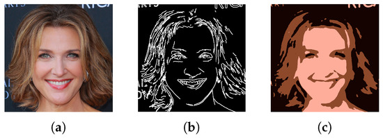
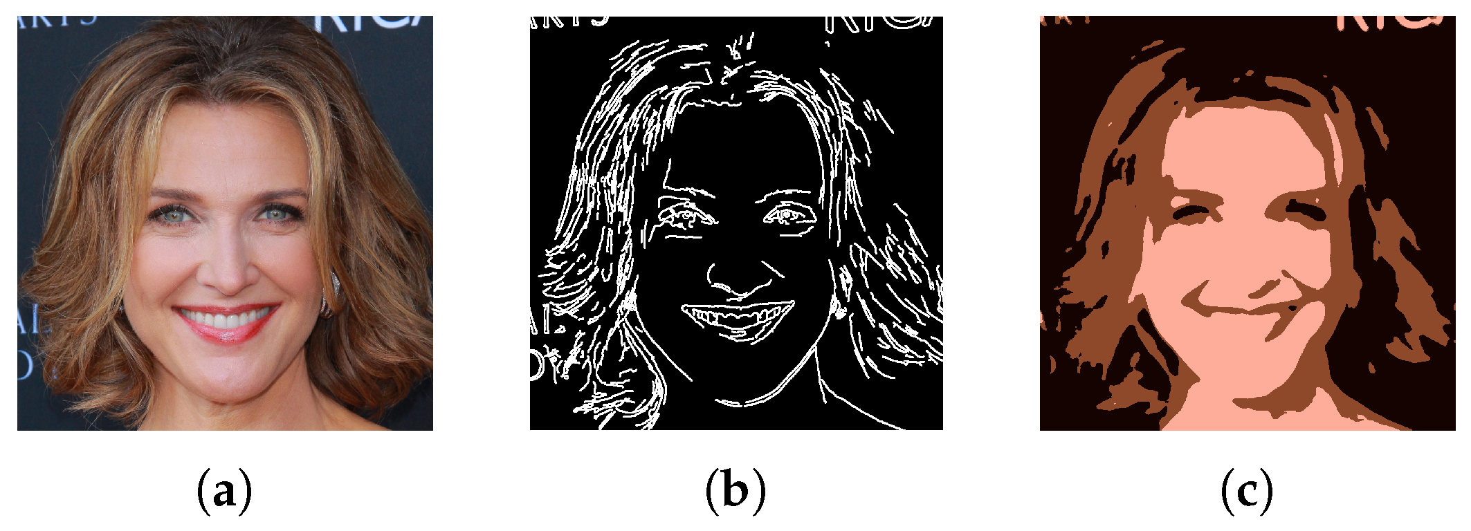
Figure 2. An example of the ground truth image and corresponding edge and color maps. (a) ground truth $I_{gt}$; (b) edge map $E_{gt}$; (c) color map $C_{gt}$.

Color maps corresponding to the style features that can provide additional information for the missing region during completion. To train $G_2$, the ground truth color maps $C_{gt}$ are created in an explicit way; they should be as simple as possible and include enough style information. First, a median filter with kernel size 21 is applied to the original images. In order to filter out the high frequency information, a large kernel size is chosen in the first median filtering. Next, the K-means algorithm with $k=3$ is used to yield the average color maps. We choose a small k because the style information should be held as much as possible. After that, a median filter with kernel size 3 is applied again to blur the sharpness of the boundary lines. A small kernel size is adopted in this median filtering because the boundary lines are thin. This results in color maps with largely constant colors in low-frequency regions; a color map example is shown in Figure 2c.

Masks play a vital role in the training. There are two types of masks that are used in the experiments: regular mask and irregular mask. Regular masks are square with a size of $128\times 128$ ($25\%$ of total image pixels) at a random location within the image. We use QD-IMD (Quick Draw Irregular Mask Dataset) as the irregular masks, as shown in Figure 3. The irregular masks are augmented by introducing four rotations ($0^{\circ }$, ${90}^{\circ }$, ${180}^{\circ }$, ${270}^{\circ }$) and a horizontal reflection for each mask.

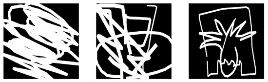
Figure 3. Irregular mask examples of the QD-IMD: Quick Draw Irregular Mask Dataset.

4.3. Training Setup and Strategy

All of the networks are trained using $256\times 256$ images with a batch size of 8 due to the machine memory. The optimization is performed employing the Adam optimizer [49] with ${\beta }_1=0$ and ${\beta }_2=0.9$, which is a stochastic optimization method with adaptive estimation of moments. For the experiments, the hyper-parameters are set to ${\lambda }_{fm,1}={\lambda }_{fm,2}=10.0$, ${\lambda }_{con}=1.0$, ${\lambda }_{pix,2}={\lambda }_{pix,3}=1.0$, ${\lambda }_{perc}=1.0$ and ${\lambda }_{adv,1}={\lambda }_{adv,2}={\lambda }_{adv,3}=0.001$. In the training processing, the stability is very important. In the edge and color model, the parameters of ${\lambda }_{fm,1}$ and ${\lambda }_{fm,2}$ should be set as having larger values than others, since the feature matching loss stabilizes the training processing. In the image completion network, its training process is more stable because it has more information including edge and color priors guiding the training. Thus, the ${\lambda }_{perc}$ should be set 1.0. All of the adversarial parameters should be set as having very small values because values that are too large tend to lead to instability in the early stage. Firstly, generators $G_1$, $G_2$ and $G_3$ are trained separately with learning rates ${10}^{-4}$ until convergence. Then, the networks are fine-tuned by removing $D_1$ and $D_2$ with learning rate ${10}^{-5}$ until convergence. Corresponding discriminators are trained with a learning rate one tenth of the generators. During each training iteration, the discriminator is trained k steps and the generator is updated once. k is set to 3 in all of the experiments. If $k<3$, the discriminators cannot distinguish the real and fake images; if $k>3$, the generators cannot get enough gradients from the discriminators. In order to stabilize the model during training, in the early stage, very small adversarial loss weights compared to the other ones are adopted, i.e., ${\lambda }_{adv,1}={\lambda }_{adv,2}={\lambda }_{adv,3}=0.001$. After that, the adversarial loss weights should be gradually increased until ${\lambda }_{adv,1}={\lambda }_{adv,2}={\lambda }_{adv,3}=1.0$, similar to the curriculum learning. The larger the adversarial parameters, the more details are generated. Thus, the adversarial parameters should be gradually increased to generate more details and keep the training process stable.

4.4. Qualitative Comparison

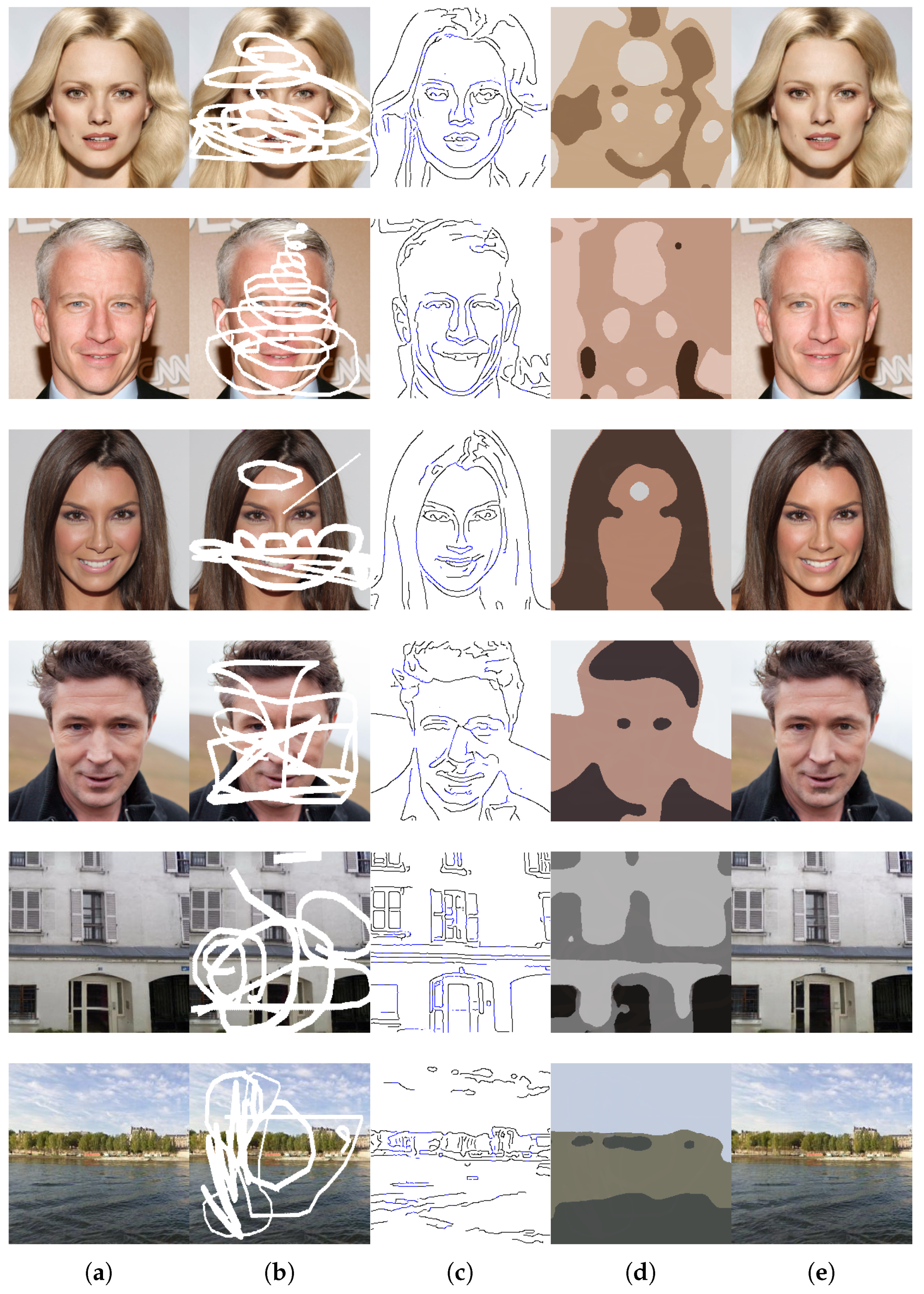
Figure 4 shows a sample of images completed by PIC-EC. For visualization, the colors of the composite edge maps $E_{comp}$ are reversed, and the generated parts are dyed blue. The PIC-EC is able to keep the image structure and color map intact with a large fraction of image damaged. Furthermore, the completed images exhibit realistic results and minimal blurriness because the edge and color generators can learn enough information to guide the image completion network.

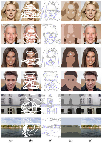
Figure 4. The images produced by PIC-EC. (a) ground truth images; (b) masked images; (c) generated edge maps by $G_1$; (d) generated color maps by $G_2$; (e) completion results without any post-processing, best viewed with zoom-in.

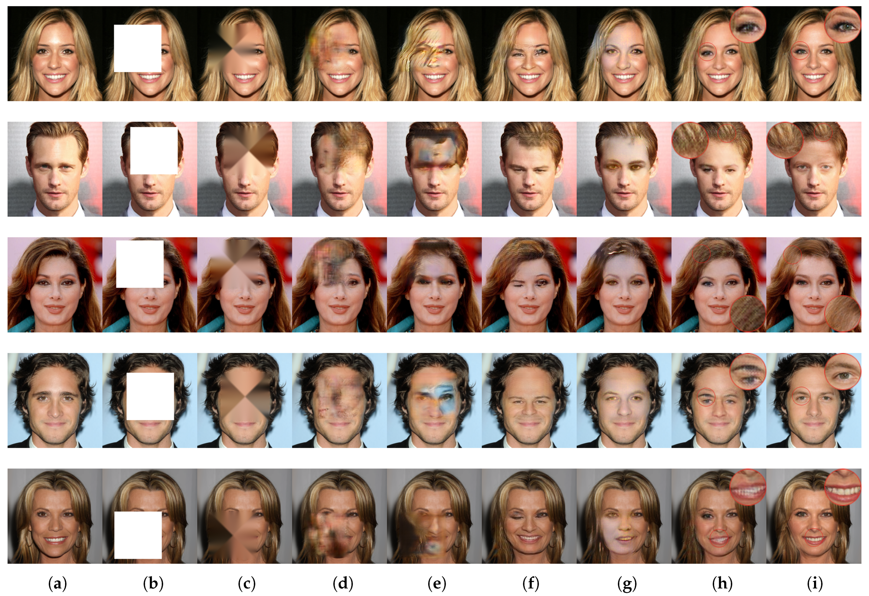
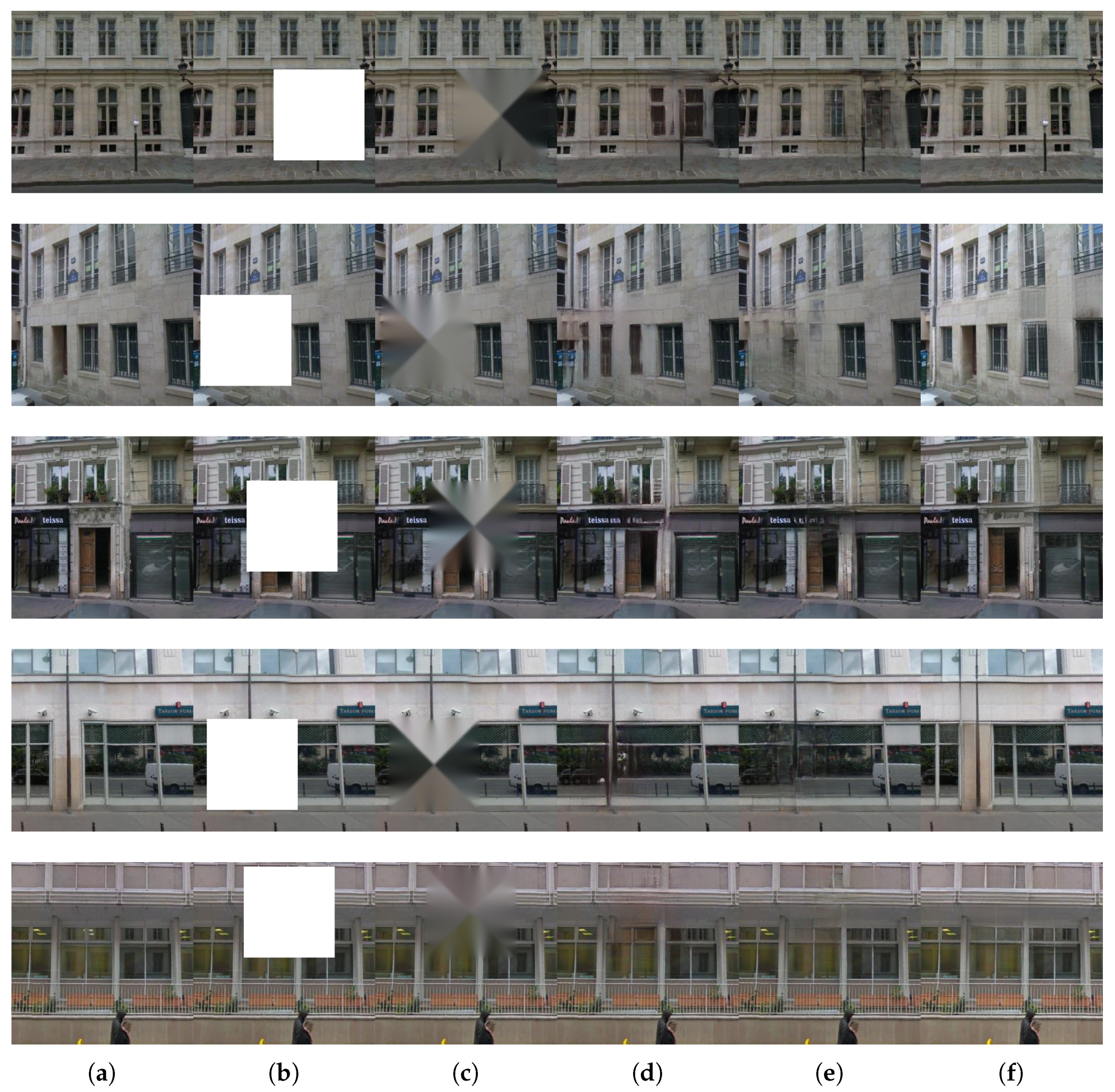
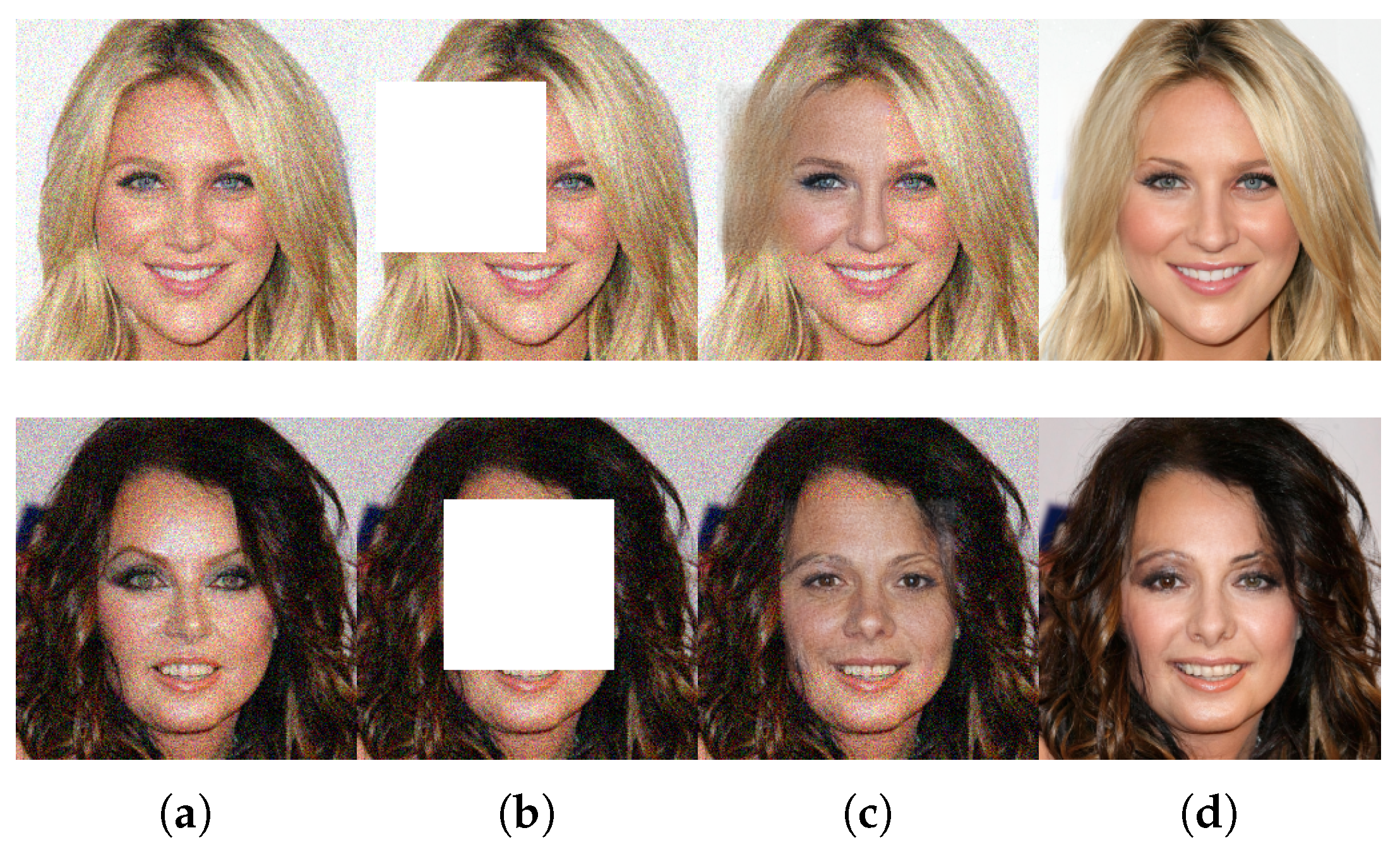
We also compare the qualitative performance of PIC-EC with the existing image completion methods using the images with irregular masks as well as the squared ones. The implementations of all these methods are based on their released source codes and pre-trained models. Note that no post-processing steps are performed for all these methods to ensure fairness of the comparisons. Figure 5 and Figure 6 summarize the qualitative comparison results on the CelebA-HQ dataset with irregular masks and squared masks, respectively. Figure 7 shows the images generated by PIC-EC with those generated by other methods on the Paris StreetView dataset with regular masks. From the results, the traditional method FMM (Fast Marching Method) [31] has no ability to generate semantic contents, especially in the larger squared mask cases, as shown in Figure 6c and Figure 7c. It is not surprising because FMM starts from the boundary of the missing region and goes inside the region gradually filling everything in the boundary using the Fast Marching Method. It takes a small neighborhood around the pixel on the neighborhood to be completed. This pixel is replaced by a normalized weighted sum of all the known pixels in this neighborhood. It does not consider the semantic relevance and is only suitable for completing the small missing regions. In Figure 5d and Figure 6d, GLCIC (Globally and Locally Consistent Image Completion) [19] shows obvious visual artifacts including blurred and distorted images in the masked regions, and it struggles to generate consistent structures with the remaining image context because of insufficient understanding of the image characteristic and ineffectiveness of convolutional neural networks in modeling long-term correlations between contextual information and the missing region. As shown in Figure 5f and Figure 6e,g, the images completed by DeepFill [36] and GMCNN [37] have severe color distortion. Therefore, these methods can not accurately fit the color distribution over CelebA-HQ dataset. Because DeepFill adopts a patch matching method in its contextual attention module, it fails to achieve plausible results even through the refinement network. In Figure 7d, GMCNN generates the distorted structures in the doors and windows. The deconvolution operations in GMCNN lead to the structure and color distortion. Although DFNet [38] shows a fine performance, it shows a lack of relevance between the hole and background regions such as symmetry of eyes, as shown in Figure 5e and Figure 6f. The images completed by the proposed method PIC-EC and the state-of-the-art method EdgeConnect [23] are closer to the ground truth than images from other methods. Both of them are able to recover correct global structures. However, the PIC-EC method can generate sharper details than EdgeConnect such as the eyes and mouth, as shown in Figure 5g,h, Figure 6h,i and Figure 7e,f. Due to EdgeConnect losing image color information when recovering the global structures, it may fill in incorrect details in some missing areas. When edge and color information is present simultaneously as the guidance, the image completion network of PIC-EC only needs to learn the fine details without having to worry about preserving image structure and color maps. Therefore, the images generated by PIC-EC demonstrate the superiority in preserving both appearance and structure coherence.

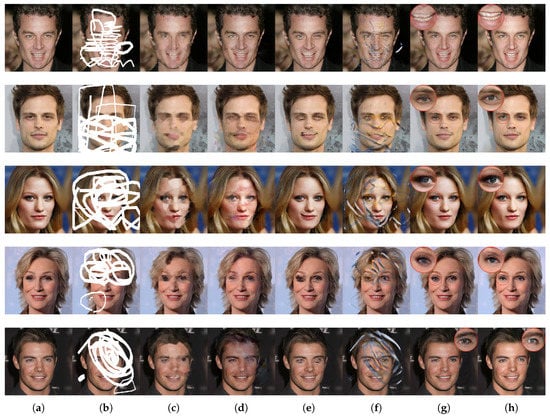
Figure 5. Comparison of qualitative results with the existing methods on irregular masked CelebA-HQ. (a) ground truth images; (b) masked input images; (c) results of the FMM [31]; (d) results of the Globally-Locally [19]; (e) results of the DFNet [38]; (f) results of the GMCNN [37]; (g) results of the EdgeConnect [23]; (h) results of the proposed method PIC-EC, best viewed with zoom-in.

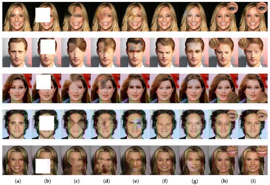
Figure 6. Comparison of qualitative results with the existing methods on random regular masked CelebA-HQ. (a) ground truth images; (b) masked input images; (c) results of the FMM [31]; (d) results of the Globally-Locally [19]; (e) results of the DeepFill [36]; (f) results of the DFNet [38]; (g) results of the GMCNN [37]; (h) results of the EdgeConnect [23]; (i) results of the proposed method PIC-EC, best viewed with zoom-in.

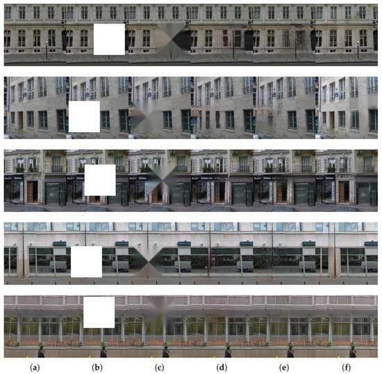
Figure 7. Comparison of qualitative results with the existing methods on random regular masked Paris StreetView. (a) ground truth images; (b) masked input images; (c) results of the FMM; (d) results of the GMCNN; (e) results of the EdgeConnect; (f) results of PIC-EC, best viewed with zoom-in.

4.5. Quantitative Comparison

In addition to the visual results, the quantitative performance of the proposed PIC-EC method is also evaluated using the following four metrics: (1) relative ${\ell }_1$; (2) peak signal-to-noise ratio (PSNR); (3) structural similarity index (SSIM) with a window size of 11 and (4) Fréchet Inception Distance (FID) [50]. PSNR directly measures the difference in pixel values and SSIM estimates the holistic similarity between two images. They assume that the ideal recovered results are exactly the same as the target images. They are the most used evaluation criteria among the image generation community. However, these two metrics assume pixel-wise independence, which may assign favorable scores to perceptually inaccurate results. Therefore, the FID metric is also used to evaluate the output quality because it is closer to human perception. FID measures the Wasserstein-2 distance between the feature space representations of real and completed images using the pretrained Inception-V3 model.

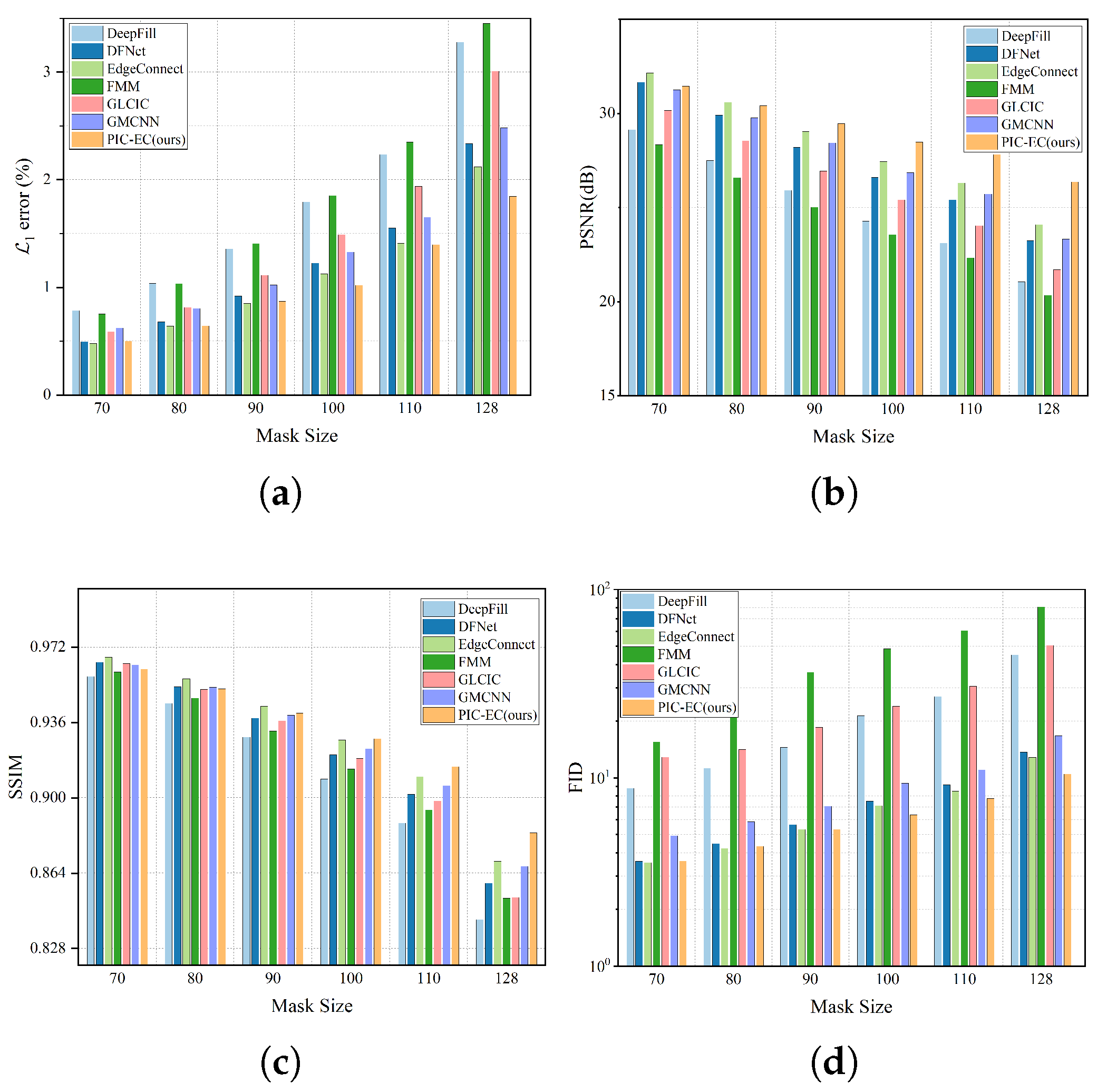
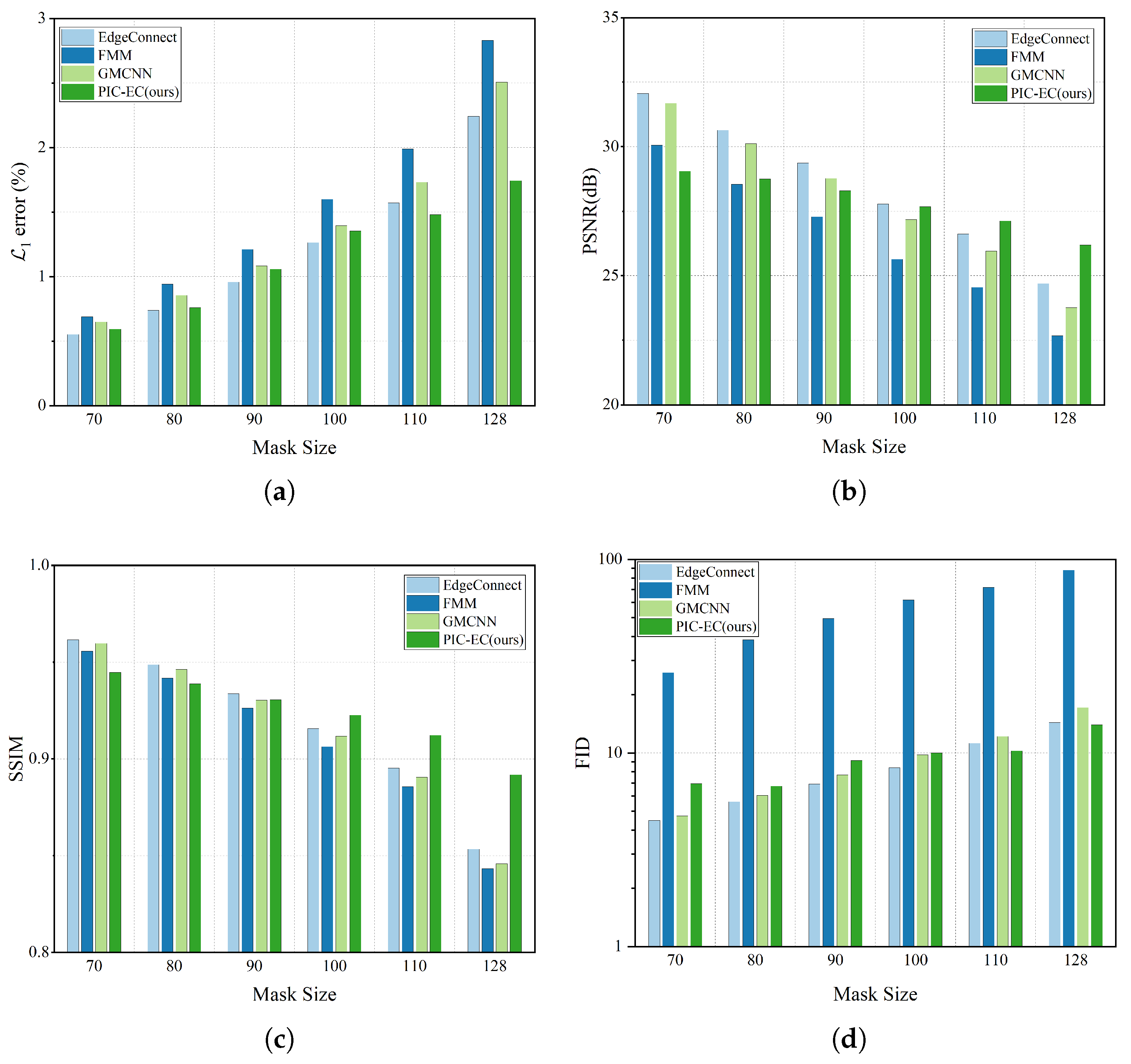
The experiment is conducted over CelebA-HQ and Paris StreetView test datasets for six different squared masks include $70\times 70$, $80\times 80$, $90\times 90$, $100\times 100$, $110\times 110$ and $128\times 128$. The location of each mask is random. We run each method on the corrupted images and get the final completed results. The statistics results are based on the completed image, which are mostly comprised of the ground truth images and are reported in Table 3 and Table 4, respectively. Figure 8 and Figure 9 show these statistics results in an intuitive way. We find that as the mask size increases, the performance of all the methods has declined gradually to varying degrees, which is in line with our intuitive experience. The methods will get less information to fill the missing region as the masks get larger. Obviously, the FMM method has the worst performance because it has no ability to generate semantic contents, especially in the larger mask cases. Overall, the EdgeConnect and PIC-EC are superior to other methods because both of them only consider making the textures of the completed images realistic, but ignore the structure and color information of the images. When the mask size is small, the performance of EdgeConnect is better than that of PIC-EC because the effect of the color map is not obvious in these cases. However, the PIC-EC method performs better than EdgeConnect in all four metrics when the mask size becomes larger, such as $110\times 110$ and $128\times 128$. In particular, PIC-EC outperforms EdgeConnect by $0.28\%$ in mean ${\ell }_1$ error, 2.273 dB in PSNR, 0.013 in SSIM and 2.384 in FID over CelebA-HQ in the largest mask size. At the same time, for Paris StreetView, PIC-EC outperforms EdgeConnect by $0.5\%$ in mean ${\ell }_1$ error, 1.4 dB in PSNR, 0.039 in SSIM and 0.377 in FID. Both PIC-EC and EdgeConnect achieve small ${\ell }_1$ error; however, the ${\ell }_1$ metric simply favors smooth and blurry results. PIC-EC has a better FID performance than EdgeConnect, which indicates that the images completed by PIC-EC are more plausible since the FID metric is closer to human perception. This should be accredited to enough prior information learned by PIC-EC. Therefore, the PIC-EC method achieves quantitative results exceeding others by a considerable margin under all the four metrics and can generate more realistic images with the guidance of edge and color maps. Other methods only consider making the textures of the completed image realistic, but ignore the structures and colors of the image. Furthermore, PIC-EC with edge guidance brings consistent improvements over others.

Table 3. Quantitative results over CelebA-HQ for six different squared masks with methods: FMM, GLCIC, DeepFill, GMCNN, DFNet, EdgeConnect and PIC-EC. Boldface in each row indicates the best performance. ${}^{*}$ Higher is better. ${}^{†}$ Lower is better. FMM: Fast Marching Method, GLCIC: Globally and Locally Consistent Image Completion, GMCNN: Generative Multi-column Convolutional Neural Networks, PIC-EC: Parallel Image Completion with Edge and Color.

	Mask Size	FMM	GLCIC	DeepFill	GMCNN	DFNet	EdgeConnect	PIC-EC (Ours)
${\ell }_1{(\%)}^{†}$	70	0.76	0.59	0.78	0.62	0.49	0.48	0.50
	80	1.04	0.81	1.04	0.81	0.68	0.64	0.65
	90	1.41	1.11	1.36	1.02	0.92	0.85	0.87
	100	1.85	1.49	1.79	1.33	1.23	1.13	1.42
	110	2.35	1.94	2.23	1.65	1.55	1.41	1.39
	128	3.45	3.01	3.28	2.48	2.34	2.12	1.84
PSNR (dB) ${}^{*}$	70	28.323	30.160	29.135	31.248	31.662	32.147	31.442
	80	26.594	28.553	27.501	29.761	29.908	30.581	30.403
	90	25.022	26.927	25.918	28.435	28.196	29.031	29.458
	100	23.561	25.401	24.272	26.848	26.603	27.443	28.475
	110	22.325	24.040	23.123	25.714	25.417	26.323	27.820
	128	20.342	21.692	21.054	23.322	23.242	24.090	26.363
SSIM ${}^{*}$	70	0.960	0.964	0.958	0.963	0.965	0.967	0.962
	80	0.948	0.952	0.945	0.953	0.953	0.957	0.952
	90	0.932	0.937	0.929	0.940	0.938	0.944	0.941
	100	0.914	0.919	0.900	0.923	0.921	0.928	0.928
	110	0.894	0.898	0.888	0.906	0.902	0.910	0.915
	128	0.852	0.852	0.842	0.867	0.859	0.870	0.883
FID ${}^{†}$	70	15.492	12.855	8.799	4.919	3.602	3.542	3.611
	80	23.370	14.138	11.233	5.841	4.468	4.220	4.323
	90	36.263	18.511	14.510	7.068	5.641	5.320	5.318
	100	48.484	23.960	21.327	9.351	7.513	7.097	6.355
	110	60.435	30.609	26.989	11.003	9.163	8.486	7.770
	128	80.859	50.313	44.917	16.695	13.659	12.820	10.436

Table 4. Quantitative results over the Paris StreetView for six different masks with methods: FMM, GMCNN, EdgeConnect and PIC-EC. Boldface in each row indicates the best performance. ${}^{*}$ Higher is better. ${}^{†}$ Lower is better.

	Mask Size	FMM	GMCNN	EdgeConnect	PIC-EC (Ours)
${\ell }_1{(\%)}^{†}$	70	0.69	0.65	0.55	0.60
	80	0.94	0.85	0.74	0.76
	90	1.21	1.08	0.96	1.06
	100	1.60	1.39	1.26	1.35
	110	1.99	1.73	1.57	1.48
	128	2.83	2.51	2.24	1.74
PSNR (dB) ${}^{*}$	70	30.061	31.685	32.06	29.05
	80	28.542	30.121	30.64	28.75
	90	27.283	28.773	29.36	28.30
	100	25.638	27.175	27.77	27.67
	110	24.556	25.955	26.61	27.12
	128	22.675	23.768	24.79	26.19
SSIM ${}^{*}$	70	0.956	0.960	0.961	0.945
	80	0.942	0.946	0.949	0.939
	90	0.926	0.930	0.934	0.930
	100	0.906	0.912	0.916	0.923
	110	0.886	0.891	0.895	0.912
	128	0.843	0.846	0.853	0.892
FID ${}^{†}$	70	26.027	4.736	4.482	6.931
	80	38.447	6.044	5.608	6.736
	90	49.446	7.693	6.922	9.151
	100	61.679	9.788	8.397	10.009
	110	71.566	12.173	11.225	10.269
	128	88.016	17.177	14.353	13.976

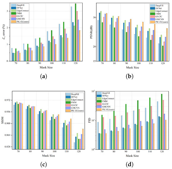
Figure 8. Effect of different masks over CelebA-HQ. (a) results of ${\ell }_1$ metric; (b) results of PSNR (Peak Signal-to-Noise Ratio) metric; (c) results of SSIM (Structural Similarity Index Metric) metric; (d) results of FID (Fréchet Inception Distance) metric.

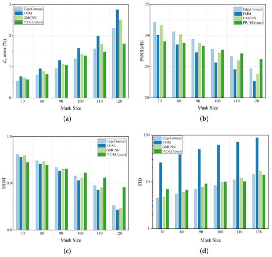
Figure 9. Effect of different masks over Paris StreetView. (a) results of ${\ell }_1$ metric; (b) results of PSNR metric; (c) results of SSIM metric; (d) results of FID metric.

4.6. Computation Time

We perform the feed-forward inference average computation time comparison for different methods. All these methods are evaluated with a machine of an Intel Core Xeon E5-2640 v3 CPU and a TITAN X (Pascal) GPU by processing 1000 $256\times 256$ images with $128\times 128$ holes. The results are listed in Table 5. DFNet achieves the shortest computation time because it only contains a smaller network than other methods. GLCIC has the longest computation time because its generation network contains much more feature map channels than other methods. Our PIC-EC method has to obtain the edge and color priors before the image completion; therefore, it takes a little more computation time. Still, PIC-EC takes less computation time than GLCIC.

Table 5. The feed-forward inference average computation time comparison for methods: GLCIC, DeepFill, GMCNN, DFNet, EdgeConnect and PIC-EC. Boldface indicates the best performance. ${}^{†}$ Lower is better.

Methods	GLCIC	DeepFill	GMCNN	DFNet	EdgeConnect	PIC-EC (ours)
Time (ms) ${}^{†}$	215.15	75.14	93.45	43.50	96.62	190.82

4.7. User Study

We perform a user study using the human perceptual metrics Two Alternative Forced Choice (2AFC) and Just Noticeable Differences (JND) over CelebA-HQ and Paris StreetView datasets. 2AFC is a method for measuring the subjective experience of a person through their pattern of choices and response times. JND is the amount something must be changed in order for a difference to be noticeable, detectable at least half the test time. In the 2AFC test, the users are asked whether or not a randomly selected completed image from each method is real. For JND, the users are asked to select the more realistic image from pairs of real and completed images. Users are given two seconds to decide for each image. This experiment is performed over 300 images for each method and mask size. The results are presented in Table 6 and Table 7. These results show that there are more images generated by PIC-EC being favored by the users because PIC-EC generates sharper images with more details.

Table 6. User study results over the CelebA-HQ for six different squared masks with methods: GLCIC, DeepFill, GMCNN, DFNet, EdgeConnect and PIC-EC. Boldface in each row indicates the best performance. ${}^{*}$ Higher is better.

	Mask Size	GLCIC	DeepFill	GMCNN	DFNet	EdgeConnect	PIC-EC (Ours)
2AFC (%) ${}^{*}$	70	37.6	67.5	70.3	76.5	87.0	85.2
	80	26.7	63.3	57.3	65.4	76.7	83.3
	90	18.7	50.7	44.7	46.6	71.3	78.3
	100	12.7	37.3	39.3	38.7	61.5	70.3
	110	7.3	18.3	31.6	22.3	50.2	66.5
	128	3.3	7.3	20.3	17.7	40.3	61.7
JND (%) ${}^{*}$	70	16.7	21.2	44.0	33.3	36.7	40.5
	80	10.0	12.5	35.7	26.7	26.7	36.7
	90	6.7	10.5	19.2	23.3	22.5	32.4
	100	4.4	9.1	15.2	16.7	18.4	28.6
	110	2.4	5.3	6.7	13.3	17.6	26.3
	128	2.0	2.6	5.1	10.0	12.5	21.2

Table 7. User study results over the Paris StreetView for six different squared masks with methods: GMCNN, EdgeConnect and PIC-EC. Boldface in each row indicates the best performance. ${}^{*}$ Higher is better.

	Mask Size	GMCNN	EdgeConnect	PIC-EC (Ours)
2AFC (%) ${}^{*}$	70	73.3	70.5	86.7
	80	68.3	67.7	83.1
	90	66.7	53.3	75.5
	100	57.4	40.4	65.0
	110	46.5	36.7	60.3
	128	40.2	28.2	57.2
JND (%) ${}^{*}$	70	38.7	41.9	45.5
	80	32.2	35.3	37.5
	90	29.1	32.5	34.4
	100	22.6	28.1	29.1
	110	16.1	24.2	26.5
	128	12.9	23.3	24.2

4.8. Limitations

Although the PIC-EC model is able to generate semantically plausible and visually pleasing contents, it has some limitations. As demonstrated in [51], deep neural networks are easily fooled by the adversarial examples. In order to explore the limitations of PIC-EC, we generate some adversarial examples by adding the Gaussian noise. Figure 10 illustrates the completion results over these adversarial examples. As Figure 10 suggests, the performance of PIC-EC is easily affected by the noise in the textured regions, such as the hair and eyes. In addition, the image tones are darker. Since PIC-EC should learn the image features from the known region, the adversarial examples will degrade the quality of features and affect the performance of PIC-EC.

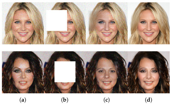
Figure 10. Completion results affected by the adversarial examples. (a) adversarial examples; (b) masked images; (c) completion results affected by noise; (d) completion results without noise.

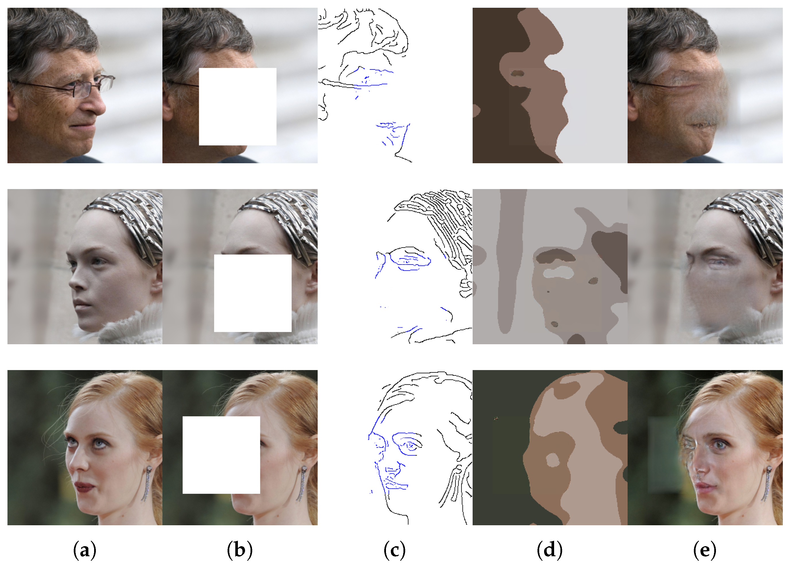
In PIC-EC, the image completion network would also be fooled by the misleading edge and color priors. Figure 11 shows some failure cases of PIC-EC. For visualization, the colors of the edge maps are reversed and the generated parts are dyed blue. As shown in Figure 11c, the edge maps in the missing region are not intactly restored. Therefore, there is not enough edge prior to construct the structure of the missing region. In this case, the color prior dominates the image completion and the completed region would be blurry because the color maps contain a lot of low-frequency information that are less affected. These failure cases indicate that PIC-EC cannot handle some unaligned faces well, especially the side face images. This issue may be alleviated with 3D data augmentation.

Figure 11. Failure cases of PIC-EC. (a) ground truth images; (b) masked images; (c) generated edge maps; (d) generated color maps; (e) completion results.

5. Discussion

Image completion is a challenging task because it is an ill-posed inverse problem and requires generating visually pleasing new pixels that are semantically consistent with the surrounding regions. Therefore, prior knowledge plays a vital role in this task to achieve meaningful and visually believable results. Under the guidance of this idea, we use both edge and color information as the prior knowledge for image completion. The results presented in the previous section have suggested that our method PIC-EC achieved superior performance on standard benchmarks, both qualitatively and quantitatively.

Figure 4 showed that $G_1$ and $G_2$ are capable of hallucinating edge and color maps in the missing regions given the rest of the image. It is essential for the following image completion task. Edge and color maps recovery is a relatively easy task compared to image completion. Thus, the image completion network only needs to synthesize the details for the missing region and this will greatly reduce the pressure on the image completion network. As illustrated in Figure 5, the qualitative comparison results over CelebA-HQ with irregular masks, our PIC-EC method performed better than other methods in terms of image structural integrity, color accuracy and texture details such as the eyes and mouth. Figure 6 and Figure 7 led to a similar conclusion. Table 3 and Table 4 and Figure 8 and Figure 9 quantitatively demonstrated comparison results for six different masks. These results suggested that, as the damaged area of the image increases, the performance of all the methods decreases. In general, this is a normal phenomenon. However, PIC-EC is minimally affected because edge and color maps can provide enough prior knowledge for the image completion network. The user study further indicated that the images synthesized by PIC-EC were closer to the ground truth images under human visual perception.

In the domain of image-to-image (I2I) translation [26,27,39], photo-realistic images can be synthesized from sparse binary edge maps by cGANs. Although the images generated by these methods were not so accurate, they suggested that the edge map is an effective prior for image generation. Existing research [52] recognizes the critical role played by the color map which can be seen as an explicit style feature in the domain of image reconstruction. It leads us into considering the introduction of the color map to improve the style consistency between the missing region and the remaining image context. Our study aims to contribute to this growing area of research by exploring the role of prior knowledge in the image completion task.

Although PIC-EC has achieved semantic plausibility and visually pleasing results, there are also some limitations existing. Firstly, PIC-EC is easily fooled by the adversarial examples that will degrade the quality of features and affect the performance of PIC-EC. Secondly, since edge and color generators are fundamental to the PIC-EC, once they are not working properly, PIC-EC fails to accurately complete the missing region. This happens sometimes in richly textured areas, or when a large portion of the side face image is missing. For this reason, improving the robustness against the adversarial examples and the performance of edge and color generators have become the important research directions in the future.

6. Conclusions

In this paper, a novel image completion method, named PIC-EC, has been proposed to solve this linear inverse problem. PIC-EC decouples the image completion problem into three easier sub-problems corresponding to the edge path, the color path and the image completion network, all of them following the adversarial model. Parallel edge and color paths are trained to hallucinate edge and color maps of the missing region, and then the following image completion network fills in the missing region using the hallucinated edge and color maps as the priors. The proposed method has been evaluated over standard benchmarks and experimental results suggest that PIC-EC has achieved superior performance compared to other methods from both qualitative and quantitative aspects.

References

- Bertalmio, M.; Sapiro, G.; Caselles, V.; Ballester, C. Image inpainting. In Proceedings of the 27th Annual Conference on Computer Graphics and Interactive Techniques, New Orleans, LA, USA, 23–28 July 2000; pp. 417–424. [Google Scholar]
- Ballester, C.; Bertalmio, M.; Caselles, V.; Sapiro, G.; Verdera, J. Filling-in by joint interpolation of vector fields and gray levels. IEEE Trans. Image Process. 2001, 10, 1200–1211. [Google Scholar] [CrossRef] [PubMed]
- Levin, A.; Zomet, A.; Weiss, Y. Learning how to inpaint from global image statistics. In Proceedings of the 9th IEEE Conference on Computer Vision, Nice, France, France, 13–16 October 2003; pp. 305–312. [Google Scholar]
- Bertalmio, M.; Vese, L.; Sapiro, G.; Osher, S. Simultaneous structure and texture image inpainting. IEEE Trans. Image Process. 2003, 12, 882–889. [Google Scholar] [CrossRef] [PubMed]
- Roth, S.; Black, M.J. Fields of experts: A framework for learning image priors. In Proceedings of the IEEE Computer Vision and Pattern Recognition, San Diego, CA, USA, 20–26 June 2005; Volume 2, pp. 860–867. [Google Scholar]
- Efros, A.A.; Leung, T. Texture Synthesis by Non-Parametric Sampling. In Proceedings of the 7th IEEE International Conference on Computer Vision, Kerkyra, Greece, 20–27 September 1999; Volume 2, pp. 1033–1038. [Google Scholar]
- Criminisi, A.; Pérez, P.; Toyama, K. Region filling and object removal by exemplar-based image inpainting. IEEE Trans. Image Process. 2004, 13, 1200–1212. [Google Scholar] [CrossRef] [PubMed]
- Wu, J.; Ruan, Q. Object removal by cross isophotes exemplar-based inpainting. In Proceedings of the IEEE 18th International Conference on Pattern Recognition (ICPR’06), Hong Kong, China, 20–24 August 2006; Volume 3, pp. 810–813. [Google Scholar]
- Wang, J.; Lu, K.; Pan, D.; He, N.; Bao, B.K. Robust object removal with an exemplar-based image inpainting approach. Neurocomputing 2014, 123, 150–155. [Google Scholar] [CrossRef]
- Jia, J.; Tang, C.-K. Inference of segmented color and texture description by tensor voting. IEEE Trans. Pattern Anal. Mach. Intell. 2004, 26, 771–786. [Google Scholar] [CrossRef] [PubMed]
- Barnes, C.; Shechtman, E.; Finkelstein, A.; Goldman, D.B. PatchMatch: A randomized correspondence algorithm for structural image editing. ACM Trans. Graph. 2009, 28, 1–11. [Google Scholar] [CrossRef]
- Wexler, Y.; Shechtman, E.; Irani, M. Space-time completion of video. IEEE Trans. Pattern Anal. Mach. Intell. 2007, 29, 463–476. [Google Scholar] [CrossRef] [PubMed]
- Xu, Z.; Sun, J. Image inpainting by patch propagation using patch sparsity. IEEE Trans. Image Process. 2010, 19, 1153–1165. [Google Scholar] [PubMed]
- Darabi, S.; Shechtman, E.; Barnes, C.; Goldman, D.B.; Sen, P. Image melding: Combining inconsistent images using patch-based synthesis. ACM Trans. Graph. 2012, 31, 82. [Google Scholar] [CrossRef]
- Hays, J.; Efros, A.A. Scene completion using millions of photographs. ACM Trans. Graph. 2007, 26, 4. [Google Scholar] [CrossRef]
- Pathak, D.; Krahenbuhl, P.; Donahue, J.; Darrell, T.; Efros, A.A. Context encoders: Feature learning by inpainting. In Proceedings of the IEEE Conference on Computer Vision and Pattern Recognition, Las Vegas, NV, USA, 27–30 June 2016; pp. 2536–2544. [Google Scholar]
- Yang, C.; Lu, X.; Zhe, L.; Shechtman, E.; Wang, O.; Hao, L. High-Resolution Image Inpainting using Multi-Scale Neural Patch Synthesis. arXiv 2016, arXiv:1611.09969. [Google Scholar]
- Denton, E.; Gross, S.; Fergus, R. Semi-supervised learning with context-conditional generative adversarial networks. arXiv 2016, arXiv:1611.06430. [Google Scholar]
- Iizuka, S.; Simo-Serra, E.; Ishikawa, H. Globally and locally consistent image completion. ACM Trans. Graph. (TOG) 2017, 36, 107. [Google Scholar] [CrossRef]
- Li, Y.; Liu, S.; Yang, J.; Yang, M.H. Generative face completion. In Proceedings of the IEEE Conference on Computer Vision and Pattern Recognition, Madison, WI, USA, 21–26 July 2017; Volume 1, p. 6. [Google Scholar]
- Yeh, R.A.; Chen, C.; Lim, T.Y.; Schwing, A.G.; Hasegawa-Johnson, M.; Do, M.N. Semantic image inpainting with deep generative models. In Proceedings of the IEEE Conference on Computer Vision and Pattern Recognition, Madison, WI, USA, 21–26 July 2017; pp. 5485–5493. [Google Scholar]
- Li, H.; Li, G.; Lin, L.; Yu, H.; Yu, Y. Context-aware semantic inpainting. IEEE Trans. Cybern. 2018, 49, 4398–4411. [Google Scholar] [CrossRef] [PubMed]
- Nazeri, K.; Ng, E.; Joseph, T.; Qureshi, F.; Ebrahimi, M. EdgeConnect: Generative Image Inpainting with Adversarial Edge Learning. arXiv 2019, arXiv:1901.00212. [Google Scholar]
- Krizhevsky, A.; Sutskever, I.; Hinton, G.E. Imagenet classification with deep convolutional neural networks. In Proceedings of the Advances in Neural Information Processing Systems, Lake Tahoe, NV, USA, 3–6 December 2012; pp. 1097–1105. [Google Scholar]
- Goodfellow, I.; Pouget-Abadie, J.; Mirza, M.; Xu, B.; Warde-Farley, D.; Ozair, S.; Courville, A.; Bengio, Y. Generative adversarial nets. In Proceedings of the Advances in Neural Information Processing Systems, Montreal, QC, Canada, 8–13 December 2014; pp. 2672–2680. [Google Scholar]
- Isola, P.; Zhu, J.Y.; Zhou, T.; Efros, A.A. Image-to-image translation with conditional adversarial networks. arXiv 2017, arXiv:1611.07004. [Google Scholar]
- Huang, X.; Liu, M.Y.; Belongie, S.; Kautz, J. Multimodal unsupervised image-to-image translation. In Proceedings of the European Conference on Computer Vision (ECCV), Munich, Germany, 8–14 September 2018; pp. 172–189. [Google Scholar]
- Karras, T.; Aila, T.; Laine, S.; Lehtinen, J. Progressive growing of gans for improved quality, stability, and variation. arXiv 2017, arXiv:1710.10196. [Google Scholar]
- Doersch, C.; Singh, S.; Gupta, A.; Sivic, J.; Efros, A. What makes paris look like paris? ACM Trans. Graph. 2012, 31, 101. [Google Scholar] [CrossRef]
- Simakov, D.; Caspi, Y.; Shechtman, E.; Irani, M. Summarizing visual data using bidirectional similarity. In Proceedings of the 2008 IEEE Conference on Computer Vision and Pattern Recognition, Anchorage, Alaska, 23–28 June 2008; pp. 1–8. [Google Scholar]
- Telea, A. An image inpainting technique based on the fast marching method. J. Graph. Tools 2004, 9, 23–34. [Google Scholar] [CrossRef]
- Mount, D.M.; Arya, S. ANN: Library for Approximate Nearest Neighbour Searching; University of Maryland: College Park, MD, USA, 1998. [Google Scholar]
- Liu, G.; Reda, F.A.; Shih, K.J.; Wang, T.C.; Tao, A.; Catanzaro, B. Image inpainting for irregular holes using partial convolutions. In Proceedings of the European Conference on Computer Vision (ECCV), Munich, Germany, 8–14 September 2018; pp. 85–100. [Google Scholar]
- Yu, J.; Lin, Z.; Yang, J.; Shen, X.; Lu, X.; Huang, T.S. Free-form image inpainting with gated convolution. arXiv 2018, arXiv:1806.03589. [Google Scholar]
- Dolhansky, B.; Canton Ferrer, C. Eye in-painting with exemplar generative adversarial networks. In Proceedings of the IEEE Conference on Computer Vision and Pattern Recognition, Long Beach, CA, USA, 16–20 June 2018; pp. 7902–7911. [Google Scholar]
- Yu, J.; Lin, Z.; Yang, J.; Shen, X.; Lu, X.; Huang, T.S. Generative Image Inpainting with Contextual Attention. In Proceedings of the IEEE Conference on Computer Vision and Pattern Recognition, Long Beach, CA, USA, 16–20 June 2018; pp. 5505–5514. [Google Scholar]
- Wang, Y.; Tao, X.; Qi, X.; Shen, X.; Jia, J. Image Inpainting via Generative Multi-column Convolutional Neural Networks. In Proceedings of the Advances in Neural Information Processing Systems, Montreal, QC, USA, 2–8 December 2018; pp. 331–340. [Google Scholar]
- Hong, X.; Xiong, P.; Ji, R.; Fan, H. Deep Fusion Network for Image Completion. arXiv 2019, arXiv:1904.08060. [Google Scholar]
- Zhu, J.Y.; Zhang, R.; Pathak, D.; Darrell, T.; Efros, A.A.; Wang, O.; Shechtman, E. Toward multimodal image-to-image translation. In Proceedings of the Advances in Neural Information Processing Systems, Long Beach, CA, USA, 4–9 December 2017; pp. 465–476. [Google Scholar]
- Johnson, J.; Alahi, A.; Li, F.-F. Perceptual losses for real-time style transfer and super-resolution. In European Conference on Computer Vision; Springer: Cham, Switzerland, 2016; pp. 694–711. [Google Scholar]
- Miyato, T.; Kataoka, T.; Koyama, M.; Yoshida, Y. Spectral normalization for generative adversarial networks. arXiv 2018, arXiv:1802.05957. [Google Scholar]
- Ulyanov, D.; Vedaldi, A.; Lempitsky, V. Improved texture networks: Maximizing quality and diversity in feed-forward stylization and texture synthesis. In Proceedings of the IEEE Conference on Computer Vision and Pattern Recognition, Honolulu, HI, USA, 21–26 July 2017; pp. 6924–6932. [Google Scholar]
- Odena, A.; Buckman, J.; Olsson, C.; Brown, T.B.; Olah, C.; Raffel, C.; Goodfellow, I. Is generator conditioning causally related to gan performance? arXiv 2018, arXiv:1802.08768. [Google Scholar]
- Zhang, H.; Goodfellow, I.; Metaxas, D.; Odena, A. Self-attention generative adversarial networks. arXiv 2018, arXiv:1805.08318. [Google Scholar]
- Lin, T.Y.; Goyal, P.; Girshick, R.; He, K.; Dollár, P. Focal loss for dense object detection. In Proceedings of the IEEE International Conference on Computer Vision, Venice, Italy, 22–29 October 2017; pp. 2980–2988. [Google Scholar]
- Mao, X.; Li, Q.; Xie, H.; Lau, R.Y.; Wang, Z.; Paul Smolley, S. Least squares generative adversarial networks. In Proceedings of the IEEE International Conference on Computer Vision, Venice, Italy, 22–29 October 2017; pp. 2794–2802. [Google Scholar]
- Liu, Z.; Luo, P.; Wang, X.; Tang, X. Deep learning face attributes in the wild. In Proceedings of the IEEE International Conference on Computer Vision, Boston, MA, USA, 7–12 June 2015; pp. 3730–3738. [Google Scholar]
- Xie, S.; Tu, Z. Holistically-nested edge detection. In Proceedings of the IEEE International Conference on Computer Vision, Boston, MA, USA, 7–12 June 2015; pp. 1395–1403. [Google Scholar]
- Kingma, D.P.; Ba, J. Adam: A method for stochastic optimization. arXiv 2014, arXiv:1412.6980. [Google Scholar]
- Heusel, M.; Ramsauer, H.; Unterthiner, T.; Nessler, B.; Hochreiter, S. Gans trained by a two time-scale update rule converge to a local nash equilibrium. In Proceedings of the Advances in Neural Information Processing Systems, Long Beach, CA, USA, 4–9 December 2017; pp. 6626–6637. [Google Scholar]
- Nguyen, A.; Yosinski, J.; Clune, J. Deep neural networks are easily fooled: High confidence predictions for unrecognizable images. In Proceedings of the IEEE Conference on Computer Vision and Pattern Recognition, Boston, MA, USA, 7–12 June 2015; pp. 427–436. [Google Scholar]
- You, S.; You, N.; Pan, M. PI-REC: Progressive Image Reconstruction Network With Edge and Color Domain. arXiv 2019, arXiv:1903.10146. [Google Scholar]
© 2019 by the authors. Licensee MDPI, Basel, Switzerland. This article is an open access article distributed under the terms and conditions of the Creative Commons Attribution (CC BY) license (http://creativecommons.org/licenses/by/4.0/).