Adaptive Leader-Follower Formation Control of Under-actuated Surface Vessels with Model Uncertainties and Input Constraints


Abstract
:1. Introduction
1.1. Motivation
1.2. Related Works
2. Problem Formulation
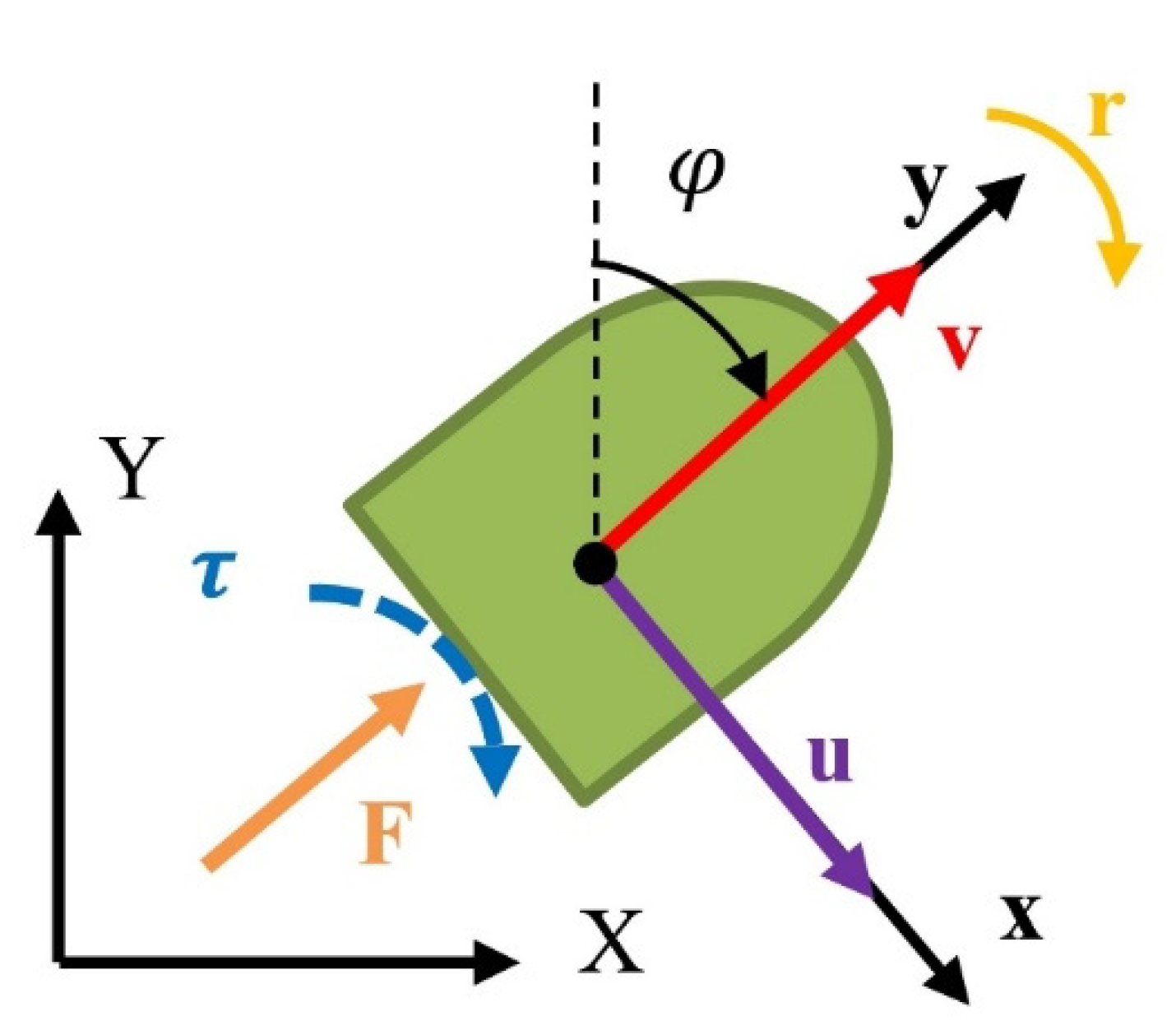
2.1. Kinematic Model of Surface Vessels
2.2. Dynamic Model of Surface Vessels
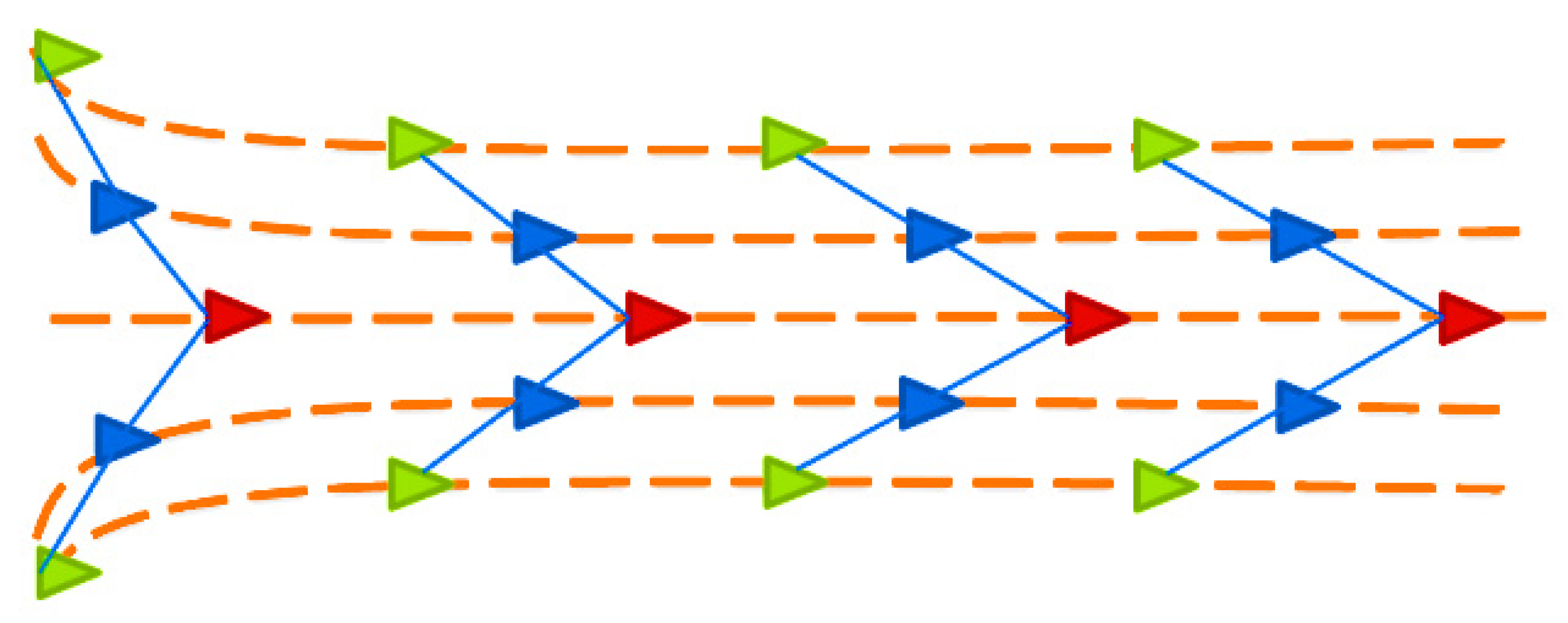
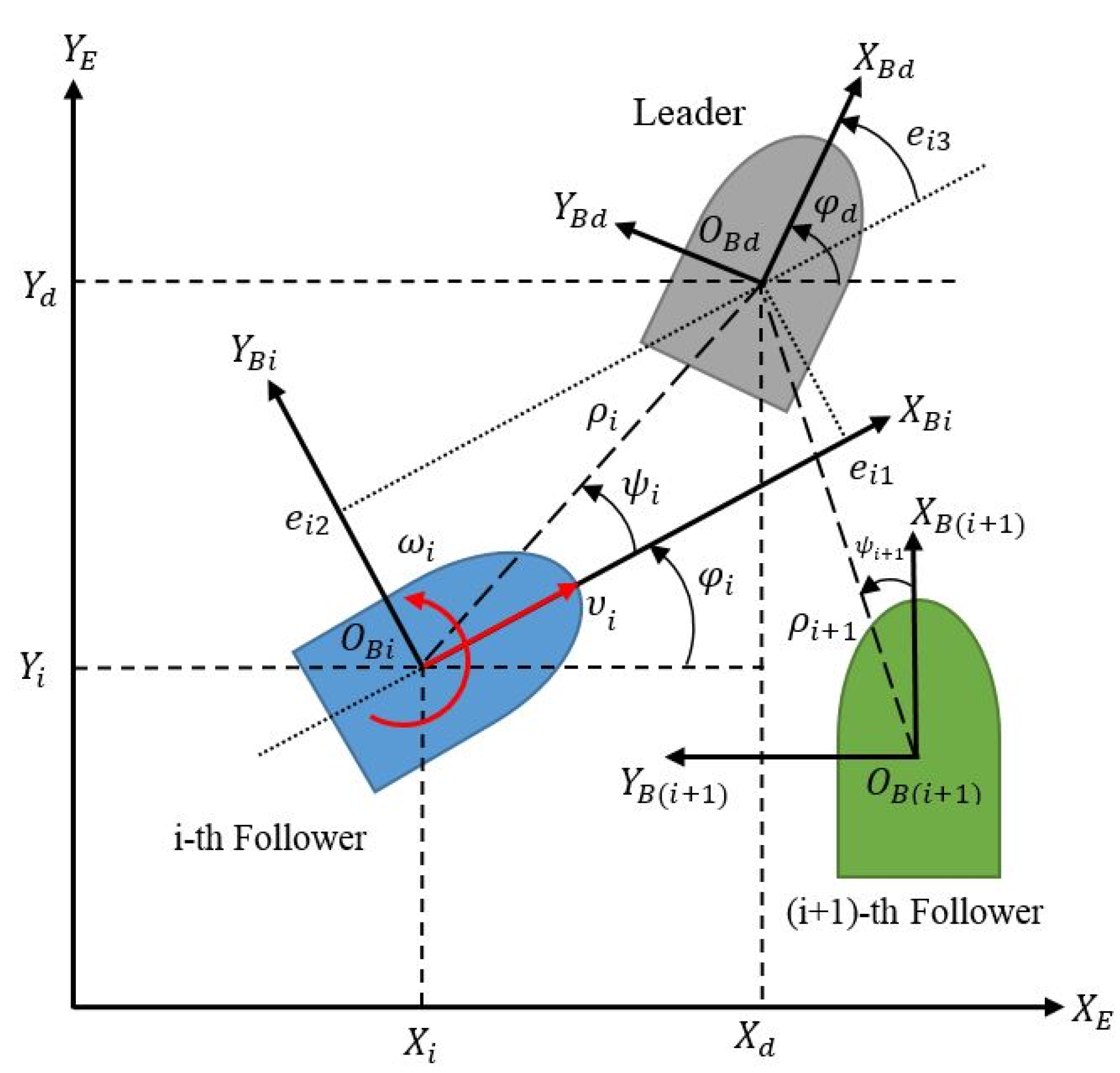
2.3. Leader-Follower Formation Model
3. Designing Adaptive-Robust Controller
3.1. Designing Adaptive-Robust Controller in the Presence of Model Uncertainties
3.2. Designing Adaptive-Robust Controller in the Presence of Model Uncertainties and Input Saturation Constraint
4. Simulation Results
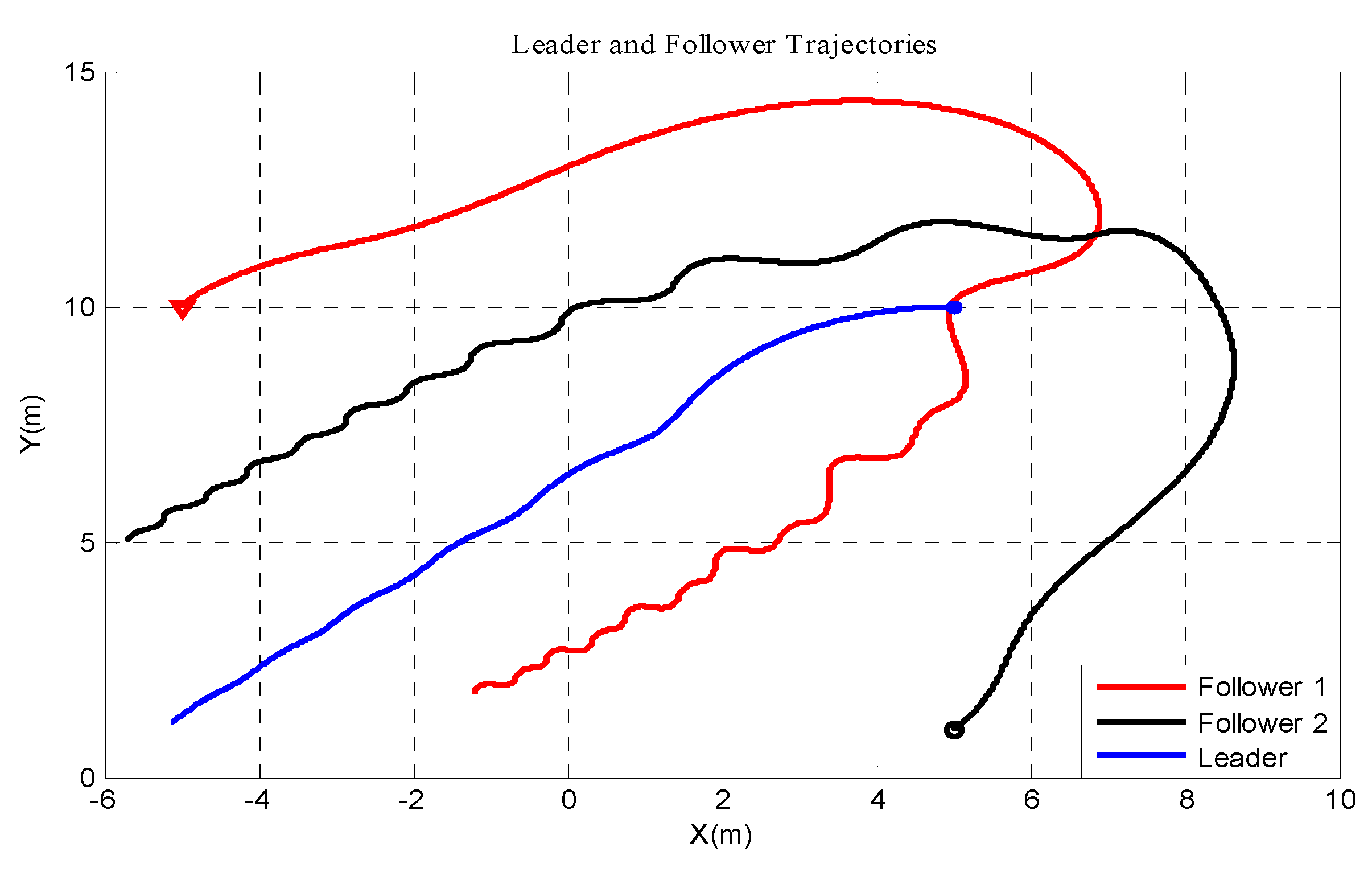
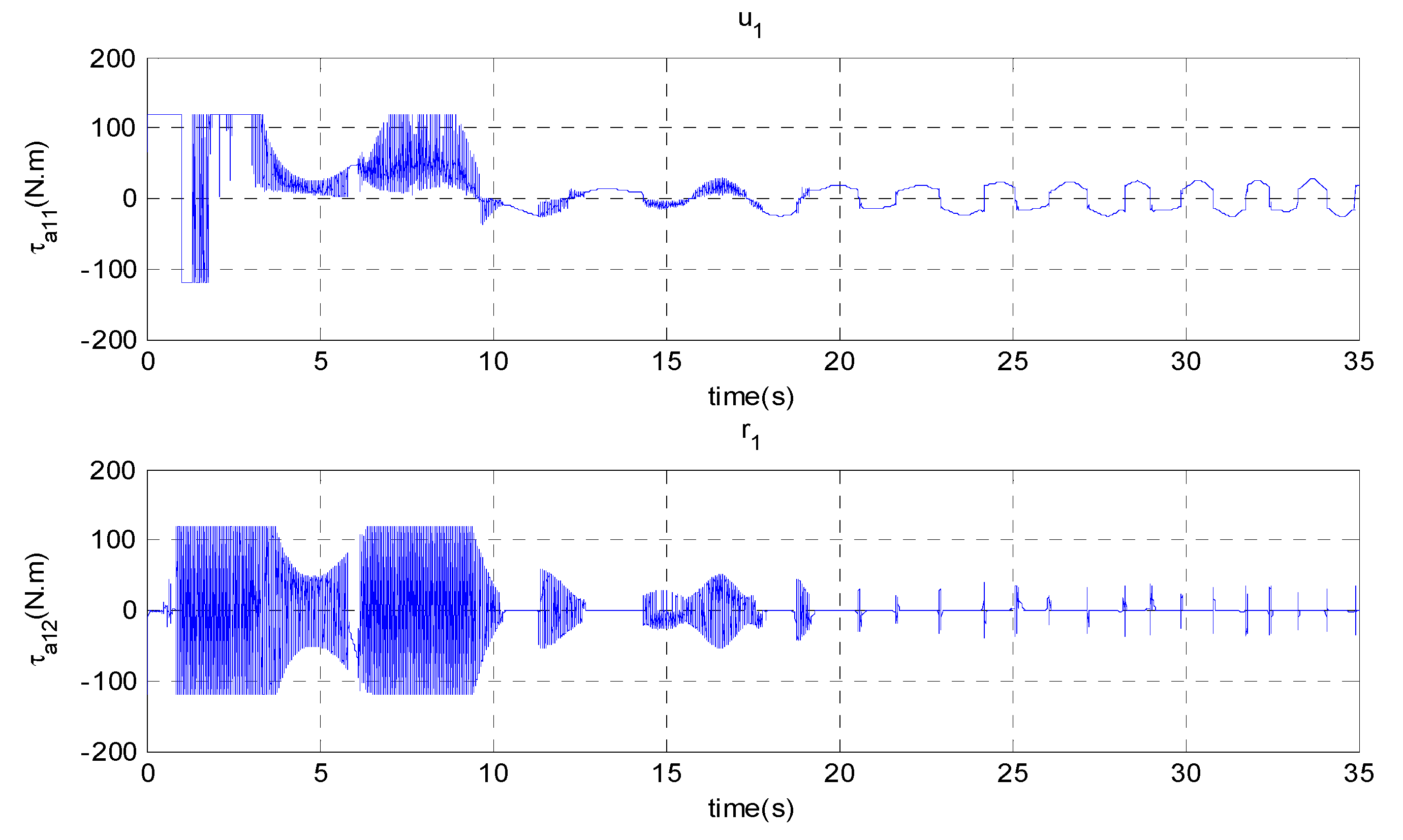
4.1. Example 1
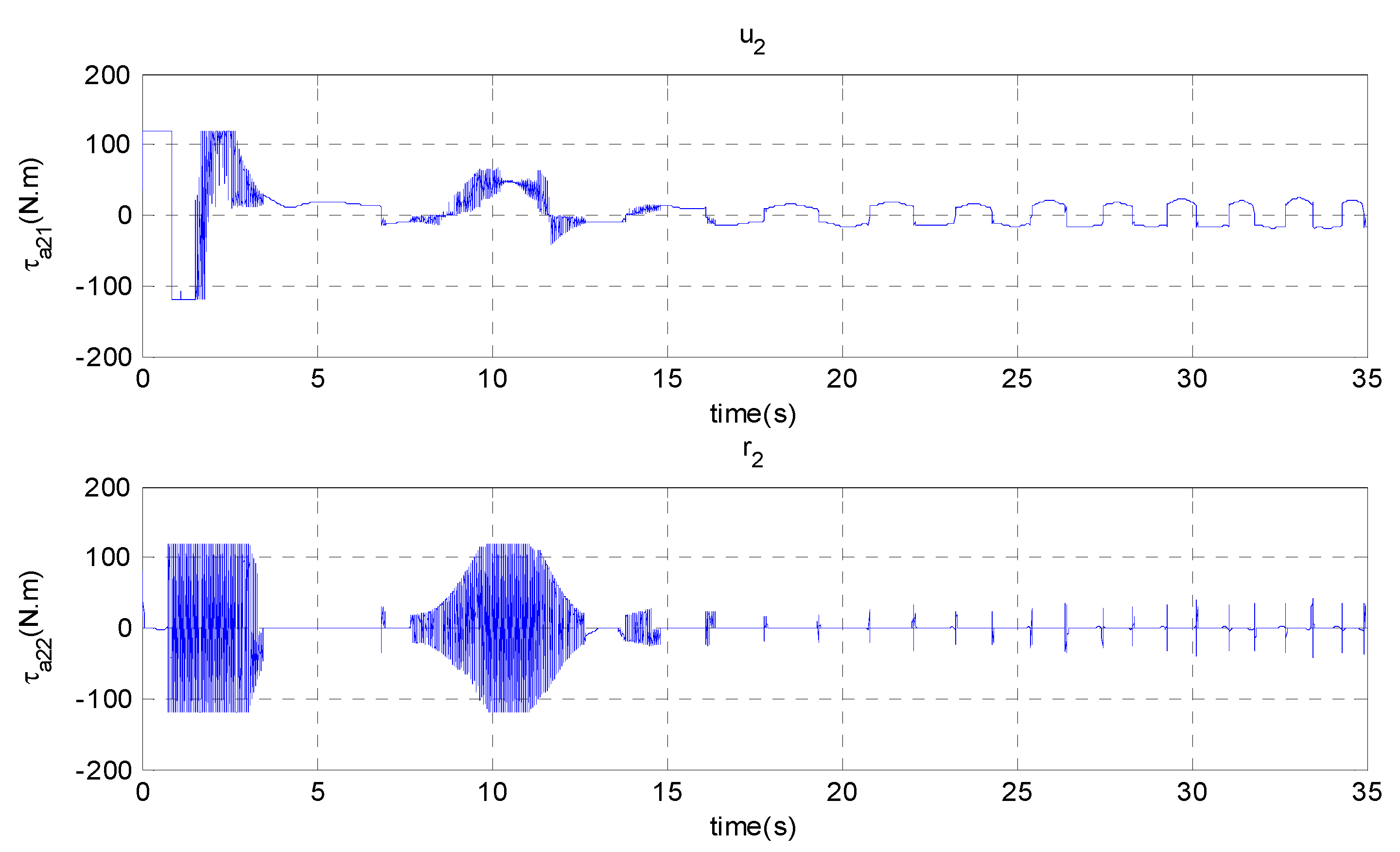
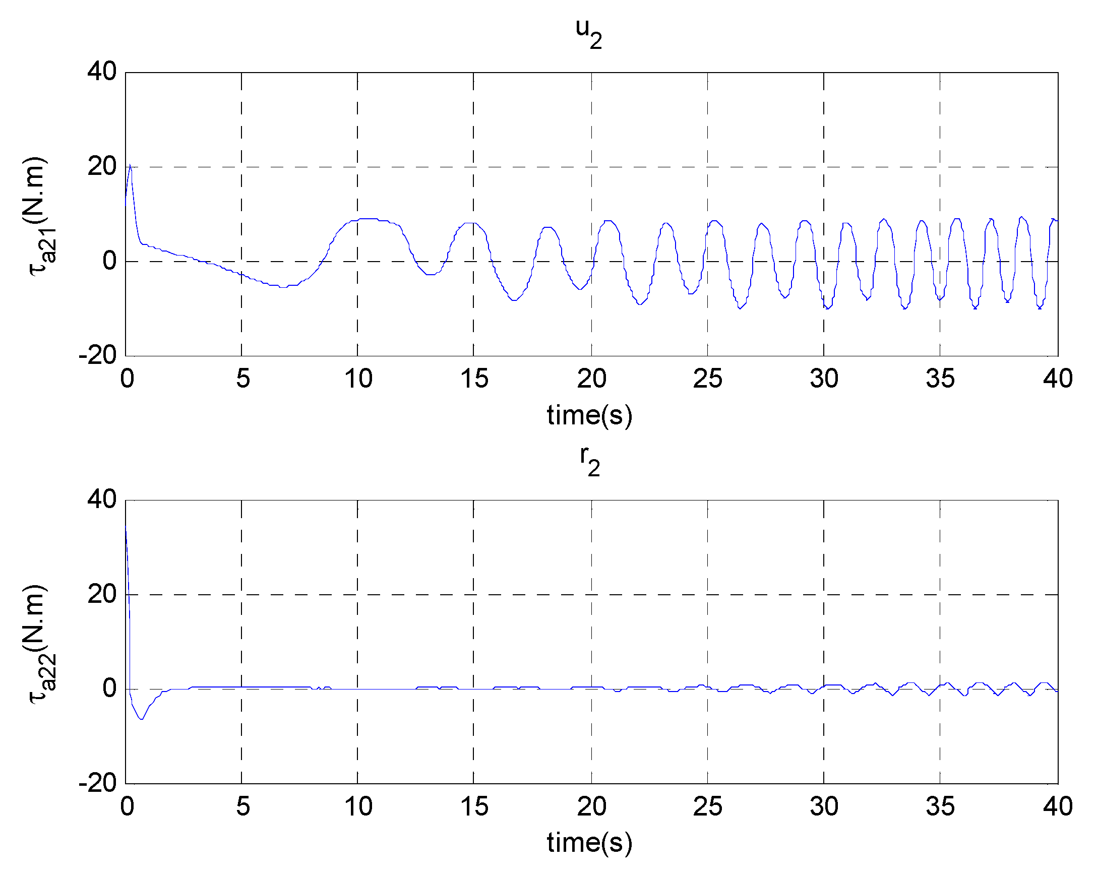
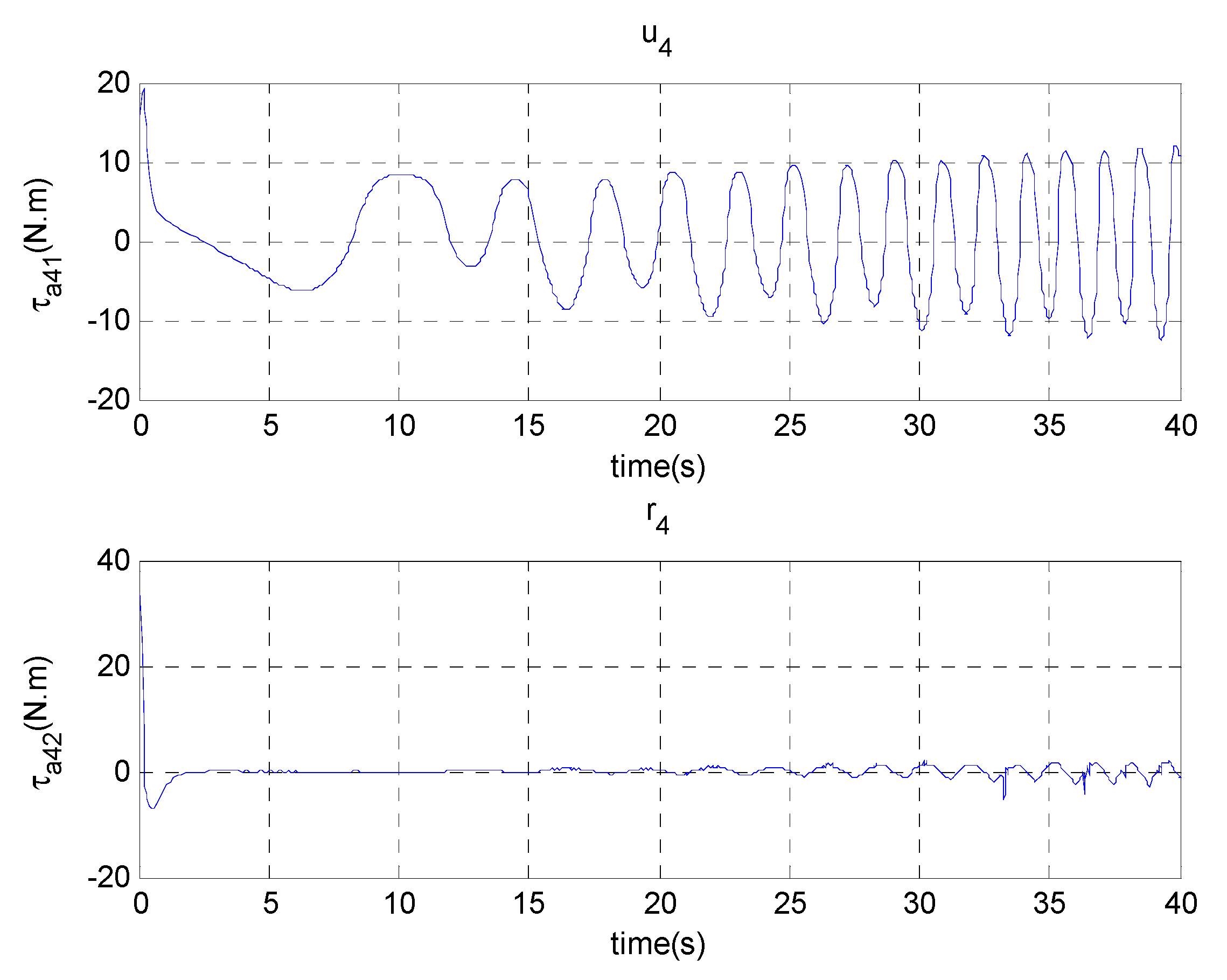
4.2. Example 2
5. Conclusions
Author Contributions
Funding
Conflicts of Interest
References
- Wang, P.K.C. Navigation strategies for multiple autonomous mobile robots moving in formation. J. Robot. Syst. 1991, 8, 177–195. [Google Scholar] [CrossRef]
- Ghabcheloo, R.; Pascoal, A.; Silvestre, C.; Carvalho, D. Coordinated motion control of multiple autonomous underwater vehicles. In Proceedings of the International Workshop Underwater Robotics, Genoa, Italy, 9–11 November 2005; pp. 41–50. [Google Scholar]
- Ihle, I.F.; Jouffroy, J.; Fossen, T.I. Formation control of marine surface craft, A Lagrangian approach. IEEE J. Ocean. Eng. 2006, 31, 922–934. [Google Scholar] [CrossRef]
- Arrichiello, F.; Chiaverini, S.; Fossen, T.I. Formation control. In Group of the Coordination and Cooperative Control; Springer: Berlin/Heidelberg, Germany, 2006. [Google Scholar]
- Breivik, M.; Subbotin, M.V.; Fosse, T.I. Kinematic aspects of guided formation control in 2D. In Groups of the Coordination and Cooperative Control; Springer: Berlin/Heidelberg, Germany, 2006. [Google Scholar]
- Das, A.; Fierro, R.; Kumar, V.; Ostrowski, J.; Spletzer, J.; Taylor, C. A vision-based formation control framework. IEEE Trans. Robot 2002, 18, 813–825. [Google Scholar] [CrossRef] [Green Version]
- Choi, K.; Yoo, S.J.; Park, J.B.; Choi, Y.H. Adaptive formation control in absence of leader’s velocity information. IET Control Theory Appl. 2010, 4, 521–528. [Google Scholar] [CrossRef]
- Zhang, J.; Jin, X.; Sun, J.; Wang, J.; Sangaiah, A.K. Spatial and semantic convolutional features for robust visual object tracking. Multimed. Tools Appl. 2018, 1–21. [Google Scholar] [CrossRef]
- Zhang, J.; Jin, X.; Sun, J.; Wang, J.; Li, K. Dual model learning combined with multiple feature selection for accurate visual tracking. IEEE Access 2019, 7, 43956–43969. [Google Scholar] [CrossRef]
- Zhang, J.; Wu, Y.; Feng, W.; Wang, J. Spatially attentive visual tracking using multi-model adaptive response fusion. IEEE Access 2019, 7, 83873–83887. [Google Scholar] [CrossRef]
- Zhang, J.; Lu, C.; Li, X.; Kim, H.J.; Wang, J. A full convolutional network based on DenseNet for remote sensing scene classification. Math. Biosci. Eng. 2019, 16, 3345–3367. [Google Scholar] [CrossRef]
- Skjetne, R.; Moi, S.; Fossen, T.I. Nonlinear formation control of marine vessel. In Proceedings of the 41st IEEE Conference on Decision and Control, Las Vegas, NV, USA, 10–13 December 2002; pp. 1699–1704. [Google Scholar]
- Cui, R.; Ge, S.S.; How, B.V.E.; Choo, Y.S. Leader-follower formation control of underactuated autonomous underwater vehicles. Ocean Eng. 2010, 37, 1491–1502. [Google Scholar] [CrossRef]
- Fossen, T.I.; Breivik, M.; Skjetne, R. Line-of-sight path following of underactuated marine craft. In Proceedings of the 6th IFAC Manoeuvring Control Marine Craft, Girona, Spain, 8 August 2003; pp. 244–249. [Google Scholar]
- Breivik, M.; Fossen, T.I. Path following of straight lines and circles for marine surface vessels. In Proceedings of the 6th IFAC Control Application Marine System, Ancona, Italy, 23 November 2004; pp. 65–70. [Google Scholar]
- Lapierre, L.; Soetanto, D.; Pascoal, A. Coordinated motion control of marine robots. In Proceedings of the 6th IFAC Conference Manoevering and Control of Marine Craft, Girona, Spain, 13 May 2003; pp. 450–464. [Google Scholar]
- Aguiar, A.P.; Ghabcheloo, R.; Pascoal, A.; Silvestre, C.; Hespanha, J.; Kaminer, I. Coordinated path-following of multiple underactuated autonomous vehicles with bidirectional communication constraints. In Proceedings of the International Symposium on Communications, Control and Signal Processing, Lisbon, Portugal, 1–6 July 2007; pp. 7–13. [Google Scholar]
- Børhaug, E.; Pavlov, A.; Pettersen, K.Y. Cross-Track Formation Control of Underactuated Autonomous Underwater Vehicles, ser. In Lecture Notes in Control and Information Systems Series; Springer: Berlin/Heidelberg, Germany, 2006; p. 336. [Google Scholar]
- Fahimi, F. Sliding mode formation control for under-actuated autonomous surface vehicles. In Proceedings of the 2006 American Control Conference, Minneapolis, MN, USA, 14–16 June 2006; pp. 4255–4260. [Google Scholar]
- Breivik, M.; Hovstein, V.E.; Fossen, T.I. Ship Formation Control: A Guided Leader-Follower Approach. IFAC Proc. Vol. 2008, 41, 16008–16014. [Google Scholar] [CrossRef] [Green Version]
- Peng, Z.H.; Wang, D.; Yao, Y.B.; Lan, W.Y.; Li, X.Q.; Sun, G. Robust adaptive formation control with autonomous surface vehicles. In Proceedings of the Chinese Control Conference, Beijing, China, 29–31 July 2010; pp. 2115–2120. [Google Scholar]
- Peng, Z.H.; Wang, D.; Lan, W.Y.; Li, X.Q.; Sun, G. Filtering robust adaptive formation guidance of unmanned surface vehicles with uncertain leader dynamics. In Proceedings of the International Conference Intelligent Control Information Processing, Dalian, China, 9 September 2010; pp. 143–148. [Google Scholar]
- Swaroop, D.; Hedrick, J.; Yip, P.; Gerdes, J. Dynamic surface control for a class of nonlinear systems. IEEE Trans. Autom. Control. 2000, 45, 1893–1899. [Google Scholar] [CrossRef] [Green Version]
- Wang, D.; Huang, J. Neural network-based adaptive dynamic surface control for a class of uncertain nonlinear systems in strict-feedback form. IEEE Trans. Neural Netw. 2005, 6, 195–202. [Google Scholar] [CrossRef] [PubMed]
- Peng, Z.; Hu, X.; Wang, D. Robust adaptive formation control of underactuated autonomous surface vehicles with uncertain dynamics. IET Control. Theory Appl. 2011, 5, 1378–1387. [Google Scholar] [CrossRef]
- Peng, Z.; Wang, J.; Wang, D. Distributed Maneuvering of Autonomous Surface Vehicles Based on Neurodynamic Optimization and Fuzzy Approximation. IEEE Trans. Control. Syst. Technol. 2017, 26, 1083–1090. [Google Scholar] [CrossRef]
- Zheng, Z.; Sun, L.; Xie, L. Error-Constrained LOS Path Following of a Surface Vessel with Actuator Saturation and Faults. IEEE Trans. Syst. Man Cybern. Syst. 2017, 48, 1794–1805. [Google Scholar] [CrossRef]
- Peng, Z.; Wang, J.; Wang, D. Containment Maneuvering of Marine Surface Vehicles with Multiple Parameterized Paths via Spatial-Temporal Decoupling. IEEE/ASME Trans. Mechatron. 2016, 22, 1026–1036. [Google Scholar] [CrossRef]
- Jin, X. Fault tolerant finite-time leader–follower formation control for autonomous surface vessels with LOS range and angle constraints. Automatica 2016, 68, 228–236. [Google Scholar] [CrossRef]
- Zheng, Z.; Huang, Y.; Xie, L.; Zhu, B. Adaptive Trajectory Tracking Control of a Fully Actuated Surface Vessel with Asymmetrically Constrained Input and Output. IEEE Trans. Control. Syst. Technol. 2017, 26, 1851–1859. [Google Scholar] [CrossRef]
- He, W.; Yin, Z.; Sun, C. Adaptive Neural Network Control of a MarineVessel With Constraints Using the Asymmetric Barrier Lyapunov Function. IEEE Trans. Cybern. 2016, 47, 1641–1651. [Google Scholar] [CrossRef]
- Zhang, J.; Lu, C.; Wang, J.; Wang, L.; Yue, X.G. Concrete cracks detection based on FCN with dilated convolution. Appl. Sci. 2019, 9, 2686. [Google Scholar] [CrossRef]
- Dai, S.; Wang, M.; Wang, C. Neural Learning Control of Marine Surface Vessels with Guaranteed Transient Tracking Performance. IEEE Trans. Ind. Electron. 2015, 63, 1717–1727. [Google Scholar] [CrossRef]
- Xiao, B.; Yang, X.; Huo, X. A Novel Disturbance Estimation Scheme for Formation Control of Ocean Surface Vessels. IEEE Trans. Ind. Electron. 2016, 64, 4994–5003. [Google Scholar] [CrossRef]
- Cui, R.; Yang, C.; Li, Y.; Sharma, S. Adaptive Neural Network Control of a MarineVessel With Constraints Using the Asymmetric Barrier Lyapunov Function. IEEE Trans. Cybern. 2017, 47, 1641–1651. [Google Scholar]
- Ghommam, J.; Saad, M. Adaptive Leader-Follower Formation Control of Underactuated Surface Vessels Under Asymmetric Range and Bearing Constraints. IEEE Trans. Veh. Technol. 2017, 67, 852–865. [Google Scholar] [CrossRef]
- Qian, D.; Tong, S.; Guo, J.; Lee, S. Leader-follower-based formation control of nonholonomic mobile robots with mismatched uncertainties via integral sliding mode. J. Syst. Control Eng. 2015, 229, 559–569. [Google Scholar] [CrossRef]
- Rostami, S.M.H.; Sangaiah, A.K.; Wang, J.; Kim, H.J. Real-time obstacle avoidance of mobile robots using state-dependent Riccati equation approach. EURASIP J. Image Video Process. 2018, 2018, 79. [Google Scholar] [CrossRef]
- Rostami, S.M.H.; Ghazaani, M. State-dependent Riccati equation tracking control for a two-link robot. J. Comput. Theor. Nanosci. 2018, 15, 1490–1494. [Google Scholar] [CrossRef]
- Rostami, S.M.H.; Ghazaani, M. Design of a Fuzzy controller for Magnetic Levitation and compared with Proportional Integral Derivative controller. J. Comput. Theor. Nanosci. 2018, 15, 3118–3125. [Google Scholar] [CrossRef]
- Ramezani, E.; Rostami, S.M.H. Fast Terminal Sliding-Mode Control with an Integral Filter Applied to a Longitudinal Axis of Flying Vehicles. J. Comput. Theor. Nanosci. 2019, 16, 1–13. [Google Scholar]
- He, S.; Xie, K.; Xie, K.; Xu, C.; Wang, J. Interference-aware Multi-source Transmission in Multi-radio and Multi-channel Wireless Network. IEEE Syst. J. 2019. [Google Scholar] [CrossRef]
- He, S.; Xie, K.; Chen, W.; Zhang, D.; Wen, J. Energy-aware Routing for SWIPT in Multi-hop Energy-constrained Wireless Network. IEEE Access 2018, 6, 17996–18008. [Google Scholar] [CrossRef]
- Zeng, D.; Dai, Y.; Li, F.; Sherratt, R.S.; Wang, J. Adversarial Learning for Distant Supervised Relation Extraction. Comput. Mater. Contin. 2018, 55, 121–136. [Google Scholar]
- Tu, Y.; Lin, Y.; Wang, J.; Kim, J.U. Semi-supervised Learning with Generative Adversarial Networks on Digital Signal Modulation Classification. Comput. Mater. Contin. 2018, 55, 243–254. [Google Scholar]
- Wang, J.; Gao, Y.; Liu, W.; Wu, W.; Lim, S.J. An Asynchronous Clustering and Mobile Data Gathering Schema based on Timer Mechanism in Wireless Sensor Networks. Comput. Mater. Contin. 2019, 58, 711–725. [Google Scholar] [CrossRef]
- Wang, J.; Gao, Y.; Liu, W.; Sangaiah, A.K.; Kim, H.J. An Intelligent Data Gathering Schema with Data Fusion Supported for Mobile Sink in WSNs. Int. J. Distrib. Sens. Netw. 2019, 15, 1550147719839581. [Google Scholar] [CrossRef]
- Wang, J.; Cao, J.; Sherratt, R.S.; Park, J.H. An improved ant colony optimization-based approach with mobile sink for wireless sensor networks. J. Supercomput. 2018, 74, 6633–6645. [Google Scholar] [CrossRef]
- Wang, J.; Gao, Y.; Yin, X.; Li, F.; Kim, H.J. An Enhanced PEGASIS Algorithm with Mobile Sink Support for Wireless Sensor Networks. Wirel. Commun. Mob. Comput. 2018, 2018, 9472075. [Google Scholar] [CrossRef]
- Salehpour, J.; Radmanesh, H.; Rostami, S.M.H.; Wang, J.; Kim, H.J. Effect of load priority modeling on the size of fuel cell as an emergency power unit in a more-electric aircraft. Appl. Sci. 2019, 9, 3241. [Google Scholar] [CrossRef]
- Rostami, S.M.H.; Sangaiah, A.K.; Wang, J.; Liu, X. Obstacle Avoidance of Mobile Robots Using Modified Artificial Potential Field Algorithm. EURASIP J. Wirel. Commun. Netw. 2019, 70, 1–22. [Google Scholar] [CrossRef]
- Peng, Z.; Wang, D.; Chen, Z.; Hu, X.; Lan, W. Adaptive Dynamic Surface Control for Formations of Autonomous Surface Vehicles with Uncertain Dynamics. IEEE Trans. Syst. Technol. 2013, 21, 513–520. [Google Scholar] [CrossRef]
- Ghazaani, M.; Rostami, S.M.H. An Intelligent Power Control Design for a Wind Turbine in Different Wind Zones Using FAST Simulator. J. Comput. Theor. Nanosci. 2019, 16, 25–38. [Google Scholar] [CrossRef]


| Parameter | Value |
|---|---|
| m11 | 25 (kg) |
| m22 | 25 (kg) |
| m33 | 2.5 (kg) |
| d11 | 7 (kg·m/s) |
| d22 | 7 (kg·m/s) |
| d33 | 5 (kg·m/s) |
© 2019 by the authors. Licensee MDPI, Basel, Switzerland. This article is an open access article distributed under the terms and conditions of the Creative Commons Attribution (CC BY) license (http://creativecommons.org/licenses/by/4.0/).
Share and Cite
Riahifard, A.; Hosseini Rostami, S.M.; Wang, J.; Kim, H.-J. Adaptive Leader-Follower Formation Control of Under-actuated Surface Vessels with Model Uncertainties and Input Constraints. Appl. Sci. 2019, 9, 3901. https://doi.org/10.3390/app9183901
Riahifard A, Hosseini Rostami SM, Wang J, Kim H-J. Adaptive Leader-Follower Formation Control of Under-actuated Surface Vessels with Model Uncertainties and Input Constraints. Applied Sciences. 2019; 9(18):3901. https://doi.org/10.3390/app9183901
Chicago/Turabian StyleRiahifard, Alireza, Seyyed Mohammad Hosseini Rostami, Jin Wang, and Hye-Jin Kim. 2019. "Adaptive Leader-Follower Formation Control of Under-actuated Surface Vessels with Model Uncertainties and Input Constraints" Applied Sciences 9, no. 18: 3901. https://doi.org/10.3390/app9183901
APA StyleRiahifard, A., Hosseini Rostami, S. M., Wang, J., & Kim, H.-J. (2019). Adaptive Leader-Follower Formation Control of Under-actuated Surface Vessels with Model Uncertainties and Input Constraints. Applied Sciences, 9(18), 3901. https://doi.org/10.3390/app9183901