Abstract
As density of a wireless LAN grows, per-user throughput degrades severely, deteriorating user experience. To improve service quality, it is important to increase system spectral efficiency. Controlling carrier-sense threshold is one of the key techniques to achieve the goal, because frequently transmissions are unnecessarily blocked by carrier sensing, even though these transmissions can take place without causing packet losses. Using high carrier-sense threshold and allowing nodes to transmit aggressively may increase the system throughput, but this approach can lead to unfair channel share and cause starvation for the edge nodes. In this paper, we propose a medium access control protocol where transmitters include the carrier-sense threshold required to protect its packet in the preamble. Nodes receiving the preamble only transmit concurrently, when they are confident that their own transmission as well as the on-going transmission will both be successfully received at the respective receivers. The simulation results show that this dual-threshold approach can achieve higher system throughput compared to using a single carrier-sense threshold, without penalizing edge nodes.
1. Introduction
IEEE 802.11-based wireless local area networks (WLANs) are widely deployed in indoor environments, providing convenient Internet connection to users. The recent trend is its densification: number of access points (APs), number of mobile devices, and amount of traffic are all rapidly increasing. In office buildings, it is easy to find tens of APs in the vicinity of a user. With increased density, the system spectral efficiency becomes a significant issue. It is important to maximize user throughput in a given space where many users are sharing channel resource.
To increase user throughput, spatial reuse (SR) must be improved: more users should be able to concurrently send packets in a given area. The problem is that concurrent transmissions could result in a packet loss, because one signal becomes interference to another signal which degrades SNR at its receiver. Therefore, current wireless LAN uses carrier sensing-based medium access control (CSMA/CA) to prevent packet collision. Before transmitting a packet, a node checks whether the channel is busy or idle. The node can transmit a packet only when it thinks the channel is idle, and defers its transmission when the channel is busy. Deciding whether the channel is busy or idle depends on the carrier-sense threshold (CST): if the node receives another signal that has a signal strength higher than CST, the node decides the channel is busy; otherwise the channel is idle.
CST is a tunable parameter, which can be independently set by each node. A node transmits conservatively when CST is low, and aggressively when CST is high. Finding optimal CST is not trivial in the systems perspective, because CST of a node not only affects throughput of the node itself, but also affects throughput of its neighboring nodes. The well-known hidden terminal and exposed terminal problems depend on CST. A high CST creates hidden terminals, whereas a low CST creates exposed terminals. Both problems are harmful for system spectral efficiency, causing packet collisions and waste of channel resource.
Until recently, a common practice was to use a fixed CST such as −82 dBm. This threshold is quite low and leads to conservative packet transmissions. When the network is sparse, avoiding packet collisions from hidden terminals is more important than promoting concurrent transmissions. However, when the network becomes dense, a low CST causes significant waste of channel resource by unnecessarily blocking nodes who can successfully send packets to their receivers.
IEEE 802.11ax, the newest WLAN standard, includes the Basic Service Set (BSS) coloring scheme to improve spatial reuse [1]. Each AP is assigned a unique ID, which is shared with its associated mobile nodes. Whenever a node transmits, the BSS ID is included in the preamble. When a node detects a preamble, it reads the BSS ID in the preamble and checks whether the incoming packet is from the same BSS or another BSS. If the packet is coming from another BSS, the node aborts receiving the packet, since it is not the destination of the packet. Moreover, the node can apply different CSTs depending on whether the packet is coming from the same BSS or a different BSS. The idea is to use a higher CST when the on-going packet is from another BSS, to transmit more aggressively and thus increase spatial reuse.
Many techniques were proposed where nodes use different CSTs depending on their positions and neighborhood conditions, instead of all nodes using a common CST. In particular, Dynamic Sensitivity Control (DSC) [2] was proposed to be included in IEEE 802.11ax, although not incorporated in the standard. The idea of DSC is to select CST based on the proximity between a mobile node and the AP. If a mobile node is placed close to the AP, it can transmit more aggressively because the SNR at the receiver can still be enough even when there is interference from other nodes. (DSC is described in more detail in the next section). The problem is that if nodes near the AP transmit aggressively, their throughput may improve, but edge nodes have less chance of transmitting on the channel. The channel share becomes unfair, and it may cause starvation to a large portion of nodes.
While nodes at the center should transmit more aggressively to improve spatial reuse, transmissions from edge nodes should also be protected. We propose a medium access control protocol where each node dynamically selects CST to protect its own transmission as well as the on-going transmission. Specifically, a transmitter includes an advertised CST in the preamble of its packet. This advertised CST should be obeyed by the neighboring nodes to protect the packet of the transmitter. When a node receives a preamble, it considers both the advertised CST, and the CST required to protect its own transmission. The node can start transmission concurrently with the on-going transmission, only when it is confident that both packets will be successfully received by their respective receivers. In the next section, we describe existing efforts on improving system spectral efficiency of wireless LANs. In Section 3, we describe the proposed protocol in detail with example scenarios to illustrate its operation. In Section 4, we evaluate performance of the proposed protocol in terms of throughput and fairness, compared to other existing protocols. Finally, in Section 5, we conclude the paper with remarks for future work.
2. Related Work
With the increase of node density and user traffic, improving system spectral efficiency has become a critical factor in servicing user needs. However, the problem of IEEE 802.11 WLAN in which the user performance significantly degrades when the network becomes dense has become well known, and the research community has proposed many different proposals to improve the system spectral efficiency of the WLANs. One line of research has focused on deriving analytical models to find the optimal CST taking account of environmental factors such as node density [3,4,5]. However, as we will discuss in the next section, a common CST cannot reuse space efficiently, as the proper CST depends on the location of the receivers as well as the senders. Although adjusting CST can improve spatial reuse, there is a limit to how much we can achieve by using a common CST.
Another approach for improving spatial reuse is to explicitly identify exposed terminals and allow them to transmit concurrently with the on-going transmission. Vutukuru et al., [6] proposed a protocol where each node maintains a Conflict Map (CMAP). The CMAP is a table that records information on which nodes should not transmit together. This table is constructed by observing packet collisions, and exchanging the information with direct neighbors. When a node overhears a packet, it decides whether it should concurrently transmit or defer transmission by looking up the CMAP. Chakraborty et al., [7] proposed CSMA/OCA, where hidden and exposed terminals are identified using Request-To-Send (RTS) and Clear-To-Send (CTS) messages. Suppose a node overhears an RTS. The node checks whether the CTS for that particular RTS is also overheard, or if the destination of the RTS is one of its neighboring nodes. If neither is true, the node thinks the RTS sender is an exposed terminal, and transmits its packet concurrently with the on-going transmission. Hosseinabadi et al., [8] proposed Concurrent-MAC, which uses a centralized approach to identify exposed terminals. In Concurrent-MAC, all nodes measure signal strengths of neighboring nodes and report the information to a central coordinator, and the coordinator computes which nodes can transmit concurrently. Once computed, the information is propagated to all nodes in the network. Whenever a node transmits a packet by winning the channel, it selects one of its nodes as a “privileged node” and includes its address in the header. When the privileged node overhears the message, it begins transmitting its packet concurrently with the other packet.
The approach that is most related to our proposed protocol is to independently select CST based on neighborhood conditions. The DSC technique proposed for IEEE 802.11ax selects CST based on proximity between the sender and the receiver, estimated using received signal strength. Specifically, the CST of a mobile node is calculated using Equation (1).
In the equation, is the CST of node i, is the RSSI of the associated AP measured at node i, and are the maximum and the minimum CST values selected by the operator, and is the margin which defines the relation between RSSI and the selected CST. According to Equation (1), nodes close to their APs will select a high CST and transmit aggressively, whereas nodes at the edge will select a low CST and transmit conservatively. Several papers report that DSC can improve system and per-user throughput compared to using a fixed CST [2,9,10,11]. However, some reports have shown that DSC can cause severe unfairness among nodes [12,13,14]; By transmitting packets aggressively, nodes close to APs get larger share of channel resource compared to cell-edge nodes. Also, aggressive nodes become hidden terminals to edge nodes, causing packet collisions and further starving the nodes. The problem of DSC is also shown in the performance evaluation section, where we compare the proposed protocol to DSC, as well as the conventional 802.11 Distributed Coordination Function (DCF).
Several proposals have been made to address the problem of DSC. Afaqui et al., [15] proposed a technique where RTS/CTS (Request-To-Send/Clear-To-Send) is adaptively used to protect cell-edge users. RTS/CTS is used only for the nodes that show high frame error rate (FER), to protect the nodes from hidden terminals. Murakami et al., [16] proposed a scheme where CST is decided based on location information of nodes. Potential hidden terminals are identified using location information, and CST is set so that the carrier-sense range covers the hidden terminals. Ropitault et al., [17] proposed a technique where transmit power and CST are adjusted based on Expected Transmission Count (ETX). The basic idea is to first calculate transmit power proportional to ETX. A high ETX means the node is experiencing bad channel condition, so the node increases transmit power to increase SNR at the receiver. Then, CST is set proportional to the transmit power. Selinis et al., [18] proposed a scheme where CST is calculated based on not only from RSSI of the associated AP, but also RSSI of neighboring APs. If the neighboring APs are closely located, the node uses a low CST to protect its transmission. Although these techniques may improve throughput and fairness of DSC, they require additional message overhead [15] or special hardware such as camera or GPS [16]. Adjusting CST based on ETX [18] may mitigate packet loss due to collisions, but edge nodes may get less chance of accessing the channel due to low CST.
There are other existing works that try to improve spatial reuse by changing parameters other than the CST such as transmit power [19] and modulation and coding scheme (MCS) [20]. Also, some works use special hardware such as directional antenna [21] or full-duplex capability [22] to improve system spectral efficiency of the system.
Compared to the existing protocols, the proposed protocol uses dual CST to effectively protect the packets that are concurrently transmitted. When there is an on-going packet, a node can only start transmitting its packet concurrently if it is confident that its own packet as well as the on-going packet will be successfully received at their respective receivers. In the next section, we describe the proposed protocol in detail.
3. Proposed Protocol
3.1. Preliminaries and Motivation
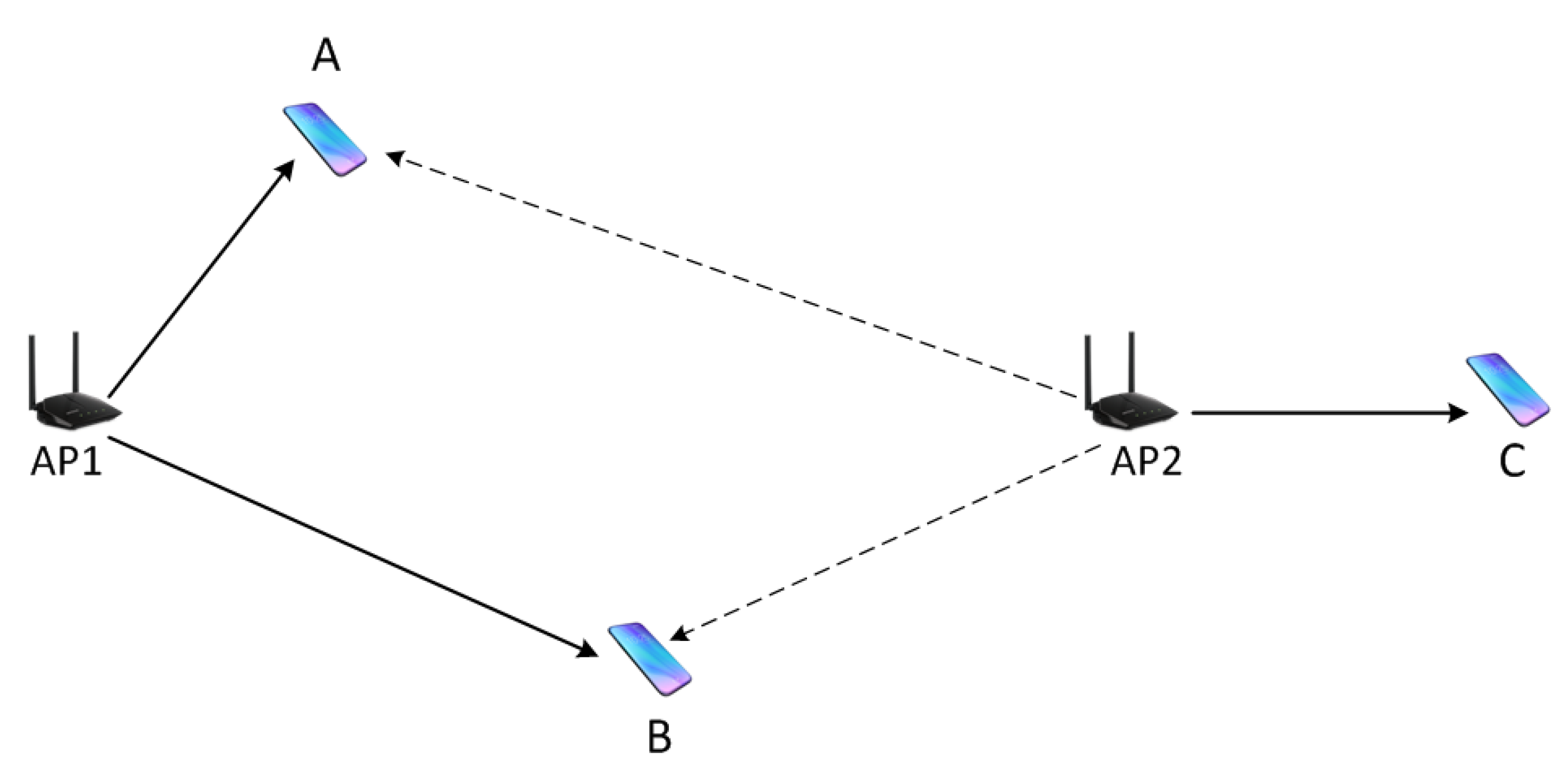
The hidden terminal problem and the exposed terminal problem are well-known problems in a carrier sensing-based medium access control protocol. The occurrence of these problems is closely related to the CST. Consider the scenario illustrated in Figure 1. Nodes A and B are associated with AP1, while node C is associated with AP2. When AP1 transmits a packet to one of its nodes, AP2 overhears the packet. If the received signal strength is higher than its CST, AP2 defers its transmission. If the signal strength is lower than the CST, AP2 will continue the channel contention process and can start transmitting its packet.
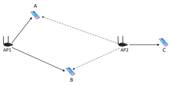
Figure 1.
An example network scenario. AP2 can transmit to node C if AP1 is transmitting to node A, but should defer its transmission if AP1 is transmitting to node B.
In this scenario, whether AP2 should actually transmit concurrently with AP1 depends on AP1’s destination. Let us assume AP2 wants to transmit a packet to node C. If AP1 is transmitting to node A, AP2 can concurrently transmit its packet, because the SNR at both node A and C are high enough to successfully decode the packet. However, if AP1 is transmitting to node B, AP2 must not transmit, because otherwise the packet transmitted by AP1 cannot be successfully decoded at B due to low SNR. The problem is that AP2 does not know where AP1’s packet is heading, nor where the destination node is placed. Thus, AP2 cannot decide whether to transmit or defer accordingly. Instead, AP2 just uses a fixed CST. If CST is set high, AP2 will transmit concurrently with AP1. If AP1 was transmitting to node B, AP2 becomes a hidden terminal causing packet collision at node B. If CST is set low, AP2 will defer its transmission. If AP1 was transmitting to node A, AP1 becomes an exposed terminal to AP2, unnecessarily preventing the transmission and degrading spatial reuse.
A proper CST should satisfy two purposes. A node should not transmit if its destination could not successfully receive the packet. Also, even if its transmission should succeed, the node should not transmit if it will cause another transmission to fail. However, the 802.11 DCF uses a fixed CST for all nodes, without considering how a transmission will affect other transmissions. Also, the DSC protocol (described in the previous section) only considers the former purpose and neglects the latter. Thus, DSC creates a lot of hidden terminals. As shown in the performance evaluation section, although DSC achieves high total throughput, it causes starvation to edge nodes and its channel share is significantly unfair.
In the above scenario, what is the best action of AP2, when it receives a preamble from AP1 and knows that AP1 is currently transmitting? If node A is the destination, AP2 can regard the channel as idle and continue backoff counting (as in DCF). If the backoff counting is over, AP2 can transmit its packet. If node B is the destination of AP1, AP2 should regard the channel as busy and pause backoff counting. Deciding whether channel is busy or idle should depend on the destination of on-going transmission. Since AP2 does not know where the on-going packet is heading, AP1 should tell AP2 (and other neighboring nodes) which node is the destination node.
There are many different ways for AP1 to inform its neighboring nodes which node is the packet destination. It can include the information in a separate message and send the message before the data packet (similar to RTS). Or, AP1 could include the information in the preamble or the MAC header of the packet. Among these design choices, we choose to include the information in the preamble. If the information is included in a separate message, control overhead becomes too large because this message should be transmitted before every data packet. If the information is included in the MAC header, a neighboring node must receive and decode the MAC header before it can cancel the reception and begin concurrent transmission. Also, usually the MAC header is encoded using the same MCS with the payload, so distant neighbors may not be able to decode the MAC header and obtain the information. Thus, it is better to include the information in the preamble.
The next design choice is on what information should be included in the preamble. Since preamble is transmitted at the lowest link rate, minimum number of bits should be used to carry the information. It is not feasible to include a 48-bit MAC address in the preamble. Thus, it is better to include an encoded CST level which should be used by the neighboring node to decide whether it should regard the channel as idle or busy. Consider the scenario in Figure 1 once again. When AP1 transmits a packet to node A, it includes in the preamble the maximum CST that must be used by the neighboring nodes, to protect its transmission. We call this CST value as advertised CST. For example, suppose AP1 knows that when it transmits a packet to node A, the received signal strength at node A will be −60 dB. Also, suppose AP1 knows that to decode the packet reliably, the SNR at node A must be at least 23 dB. Then, it means the maximum interference that can be tolerated at node A is approximately −83 dBm (neglecting the noise floor.) Thus, AP1 should block any neighboring nodes that can cause interference at node A at a strength higher than −83 dBm. AP1 should select the advertised CST so that these candidate interfering nodes find the channel busy after receiving the preamble. By including CST instead of MAC address, we can use smaller number of bits in the preamble. For example, 6 bits can be allocated to the advertised CST, which can represent 64 different values. It will be sufficient to indicate the advertised CST, ranging from −99 dBm to −36 dBm. If fewer bits are available, quantization can be used to further reduce the size of information at the cost of degraded accuracy. We propose two methods for selecting the CST; model-based scheme and measurement-based scheme. We describe the two schemes in the next sections.
3.2. Model-Based Dynamic CST Control
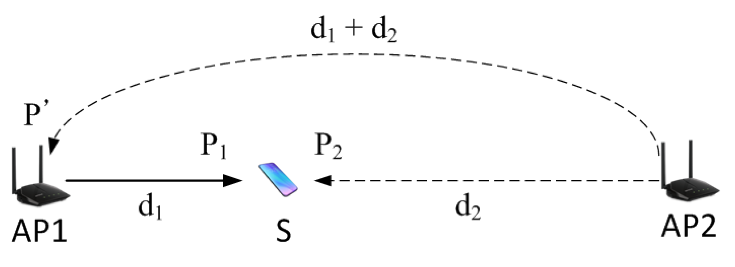
In the model-based scheme, the CST required for protecting the transmission is calculated using a path loss model. For example, a log-distance path loss model can be used. Consider the scenario shown in Figure 2. AP1 is trying to send a packet to node S. The advertised CST should be low enough to block all nodes that can potentially interfere with the transmission at the receiver. A potential interferer is a node that can cause SNR at node S to drop below the required SNR to decode the packet.
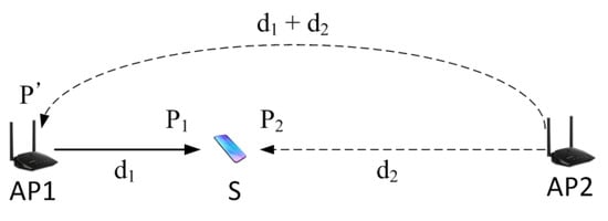
Figure 2.
An example network scenario for calculating CST. Distance between the transmitting node and the interfering node is estimated based on a pathloss model, and CST is calculated based on the distance.
Suppose is the received signal strength when the packet from AP1 arrives at node S, and is the SNR required to reliably decode a packet. Also, suppose another node AP2 transmits concurrently with AP1, so its signal becomes an interference at node S, and the interference strength is . For the AP1’s packet to be successfully decoded at node S, the following equation should hold. (We ignore the noise floor here, but the noise floor is considered in the simulations). Please note that all values are in dB scale.
We want to find the minimum interference level , which will make the packet reception fail at node S. We can calculate the minimum that destroys the packet by converting the inequality in Equation (2) to equality. To calculate the minimum , AP1 must know , assuming is fixed and known. There are two ways to obtain . First, node A constantly measures the RSSI of AP1, and send the information to AP1. Second, AP1 measures RSSI of node A whenever A transmits a packet, and assume that the links are symmetric and use that value as . Regardless of the methods, AP1 can obtain and thus calculate using Equation (3).
There are multiple positions of the interferer where the interference level at node S is . Among the positions, the farthest point from AP1 is at the opposite direction from node S. Let us assume there is an interferer AP2 placed at that position, as illustrated in Figure 2. Now, our goal is to calculate the RSSI of AP1, measured at AP2. We use the log-distance model, which calculates path loss according to the following equation.
In the equation, is the path loss, is the reference path loss, d is the distance between the sender and the receiver, is the reference distance, is the path loss exponent reflecting the environment, and is a random variable accounting for channel variations such as fading. Using the model, we define the following two functions. (We set to 0, and use the margin parameter to account for channel variations).
converts distance to path loss, whereas estimates distance from path loss. Suppose the distance between AP1 and node S is , and the distance between AP2 and node S is . Using the function, we calculate estimated values of and .
In the equations, is the transmit power, which we assume is fixed and the same for every node. and are the path loss between AP1 and S, and AP2 and S, respectively. Since AP2 is at the opposite position of AP1 from node S, the distance between AP1 and AP2 is . Thus, we can calculate the received signal strength of AP1 at AP2 () using the function as follows.
Since AP2 must be blocked when AP1 is transmitting, AP1 selects as the maximum CST that can protect its transmission. Thus, the advertised CST () is calculated as follows.
In the equation, is the margin parameter. The margin parameter is necessary for various reasons. First, it accounts for the mismatch between the model and the real path loss, caused by factors such as fading effects. Also, the calculated CST is based on assumption that there is a single interferer. In practice, there could be multiple nodes transmitting concurrently, which will increase the interference at the receiver. Since it is difficult to predict how many transmissions will take place near the receiver, we use the margin parameter to account for the possibility of multiple interferers. In this paper, we use a fixed margin that is common for all nodes. However, it could be better to select the margin for each node independently, based on the conditions around the node. For example, a larger margin could be used if the node is experiencing large amount of channel variation, and a smaller margin can be used if the channel condition is more stable. Also, a larger margin could be used for a node positioned in a dense environment, compared to a node positioned in a sparse environment. Dynamically selecting margin based on the current environment is a challenging but important issue in terms of achieving high spectral efficiency, and is left as a future work.
We return to the example scenario in Figure 1 to continue describing the proposed protocol. Suppose AP1 has calculated the advertised CST and transmitted a packet. When AP2 receives the preamble, it should consider two things before concurrently transmitting its packet with AP1. First, the RSSI of AP1 should be higher than the advertised CST, to protect the on-going transmission. Second, the on-going transmission should not destroy the packet transmitted from AP2 at node C. To find out, AP2 calculates the required CST () that will protect its own transmission. The calculation process is identical to how AP1 calculated . Then, the CST of AP2 at the moment is selected as the minimum of and .
If the current interference level is lower than , AP2 decides the channel is idle and may begin transmitting a packet to its destination. Please note that both and depends on the destinations of the potential concurrent transmitters.
In the scenario, suppose when AP1 transmits a packet, the received signal strength at AP2 is −80 dBm. In the first case, AP1 sends a packet to A. Using the described model-based method, AP1 calculates as −75 dBm, and includes the information in the preamble of the packet. When AP2 receives the preamble, AP2 was waiting for the channel to send a packet to node C. calculated at AP2 is −60 dBm. Since is higher than −80 dBm, AP2 decides the channels is idle and continues counting down the backoff counter. If the counter reaches zero, AP2 transmits concurrently with the on-going transmission from AP1. In the second case, AP1 sends a packet to B. In this case, the is calculated as −85 dBm, because node B is distant from AP1. When AP2 receives the preamble from AP1, its CST becomes = −85 dBm, which is lower than −80 dBm. Thus, AP2 decides the channel is busy and defers transmission. In summary, the proposed scheme can control CST considering not only the senders but their destinations, to improve spatial reuse while avoiding hidden terminal effects.
3.3. Measurement-Based Dynamic CST Control
The model-based CST control scheme has two weaknesses. First, the path loss model may not reflect the real environment. Even with the margin, the error in the model could lead to a CST that makes nodes transmit too conservatively or too aggressively. Second, the model-based CST assumes the worst-case scenario, where the interferer is assumed to exist at the position farthest from the transmitting node. This could make the CST low and limit the spatial reuse. In the measurement-based dynamic CST control, we do not use a path loss model, but use neighbor information exchanged as control messages between the nodes.
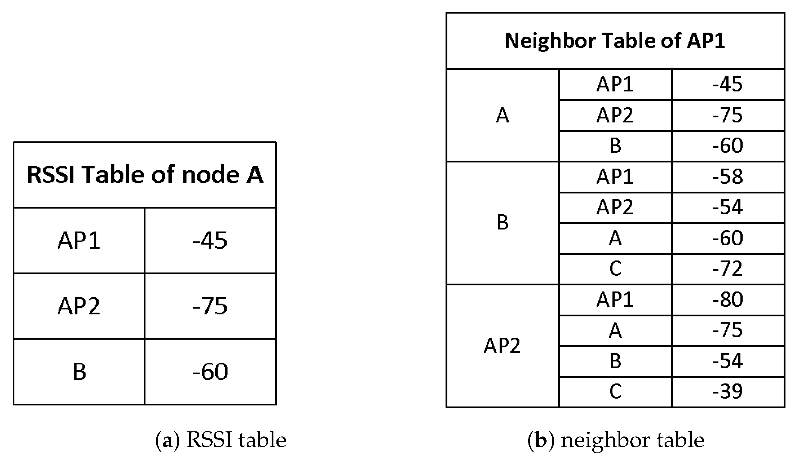
Let us consider the example scenario shown in Figure 2. In the scenario, AP1 wants to send a packet to node A, and thus it needs to calculate the advertised CST to protect the transmission. To select the advertised CST, AP1 must know the potential interferers of node A. In the measurement-based scheme, node A sends this information to AP1 in a message. To do that, each node collects RSSI of neighboring nodes whenever it overhears their message, and maintains the RSSI information using weighted moving average (WMA) in an RSSI table. For example, node A maintains the average RSSI of AP1, AP2, and node B, as in Figure 3a. (Assume node C is too far away and its signal does not reach node A.) Periodically, each node broadcasts its RSSI table to its neighbors in a control message, which is transmitted at the lowest data rate. When a node receives an RSSI table from its neighbor, it updates its neighbor table with the information. An example neighbor table of AP1 is described in Figure 3b.
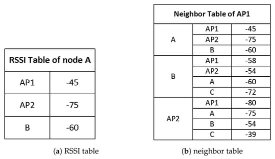
Figure 3.
An RSSI table (a) and a neighbor table (b) used in measurement-based dynamic CST control. The RSSI table maintains average RSSI values for each of the neighbors. Also, the RSSI tables are periodically exchanged between neighboring nodes. Whenever a node receives an RSSI table from the neighbor, it updates the neighbor table which records the RSSI table of each neighbor.
Using the neighbor table, AP1 finds out that when it transmits, the received signal strength at node A will be −45 dBm. If the required SNR threshold is 23 dB, the interference level at node A should be less than −68 dBm. Looking at the neighbor table, the expected interference level at node A when AP2 transmits is −75 dBm, which is less than −68 dBm. Thus, AP1 does not need to block AP2. However, if node B transmits, the SNR at node A becomes less than 23 dB and the packet will not be successfully decoded. Therefore, node B becomes the potential interferer for AP1 transmitting to node A. To block node B, AP1 sets the advertised CST as −58 dBm -. When AP2 receives the preamble from AP1, it finds out that its transmission will not destroy the on-going transmission. Now, AP2 looks at its neighbor table to find out if when AP2 transmits a packet to node C, it will be successfully decoded at node C. If the packet is expected to survive, AP2 decides the channel is idle.
Suppose AP1 wants to transmit its packet to node B. Consulting the neighbor table, AP1 finds that both node A and node AP2 are potential interferers. In this case, the advertised CST is selected based on the farthest interferer, which is AP2 in this case. Thus, the advertised CST becomes −80dBm - , to prevent AP2 from transmitting. When AP2 receives the preamble, it measures the RSSI and reads the advertised CST. Since the RSSI is higher than the advertised CST, AP2 decides the channel is busy and defers its transmission.
Please note that the margin parameter is also used in the measurement-based scheme. Although the scheme does not use a path loss model to calculate CST, margin is still needed because of channel variations, and possibility of multiple interferers. While the model-based scheme selects CST conservatively by assuming that an interferer exists in the worst position, the measurement-based scheme could choose a CST which makes the nodes transmit more aggressively. Because of that, a larger may be needed for measurement-based scheme to account for multiple interferers, compared to the model-based scheme. In the evaluations, we study the performance of protocols while varying the margin value.
4. Performance Evaluation
4.1. Simulation Setup
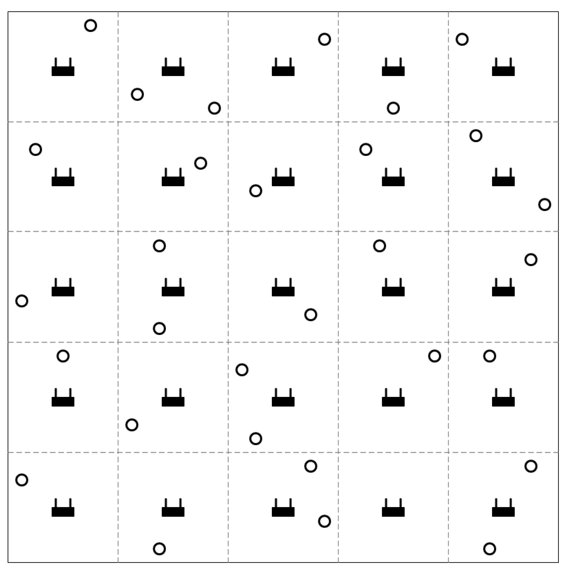
Performance of the proposed protocol was evaluated using the ns-3 simulator [23]. In a 100 m × 100 m area, APs are placed in a grid topology, and mobile nodes are randomly deployed (as shown in Figure 4). Once deployed, each mobile node selects and associates with an AP after scanning the area for beacons. In the simulations, we assume that every mobile node has a downlink traffic to receive from the AP. We use UDP traffic with 1472 bytes of packet size, and the MCS is set so that the link speed is 54 Mbps. For the path loss model, we use the log-distance model. We use the default values used in ns-3 for the parameters in the path loss model; the reference distance () is 1 m, the reference path loss () is 46.67 dB, and the path loss exponent () is 3. Transmit power and noise floor are set to 20 dBm and −93.97 dBm, respectively. We compare four different techniques. The first one is denoted as “Legacy”, which is the conventional IEEE 802.11 DCF with fixed CST, which is set to −82 dBm. The second one is “DSC”, which selects CST considering the proximity between pair of communicating nodes. For the parameters of DSC (shown in Equation (1)), and are set to −99 dBm and −39 dBm, and was set to 25 dBm [2]. The third and the fourth schemes are the ones proposed in the paper. The third one, “Model-based”, uses the path loss model to calculate the CST which is advertised in the preamble. The model-based scheme uses the log-distance path loss model, with = 3. The fourth one, called “Measurement-based” uses neighbor information exchanged through control messages to decide the advertised CST. For both schemes of the proposed protocol, the margin parameter is set to 6 dB.
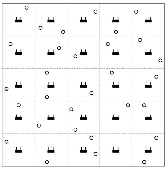
Figure 4.
An example simulation environment. The APs are placed in a grid topology and the mobile nodes are randomly deployed in the area.
To evaluate performance, we use the following metrics. First, we measure the total throughput, which is the number of data bits successfully transferred in the network per second. With the same number of nodes and the same amount of traffic, higher spatial reuse will lead to more bits transferred in the same time period. Second, we measure the bottom 25% throughput. We sort the node throughput in the ascending order, and select 25% of the nodes with the least throughput. The bottom 25% throughput is the aggregate throughput of these nodes. As discussed earlier, a system can increase total throughput by letting a small subset of node dominate the channel, which leads to starvation for most of the other nodes. If protocol A achieves higher total throughput than protocol B but gets lower bottom 25% throughput, we cannot say that protocol A outperforms protocol B. On the other hand, if protocol A achieves higher number for both the total throughput and the bottom 25% throughput compared to protocol B, it is more probable that protocol A is reusing the space more effectively than protocol B. Third, we measure Jain’s fairness index [24], which is a more direct metric used to measure fairness of a system. The equation for Jain’s fairness index is shown in Equation (12). In the equation, is the throughput of node i, and n is the total number of nodes.
Fourth, we measure the delivery ratio of the system. Delivery ratio is calculated as the number of successfully received packets divided by number of transmitted packets. Packet losses can occur because of packet collisions, which are caused from two major reasons. First, since the wireless LAN uses random backoff for channel contention, it is possible that multiple nodes could finish counting down their backoff counters and start transmissions simultaneously. Other than that, packet collisions are caused by hidden terminals, which is related to CST. If CSTs are not properly set, it could create hidden terminals which increases packet collisions and decrease the delivery ratio.
To obtain each point in the result graph, we ran 100 simulations with different topology and different seed for the random number generator, and averaged the results.
4.2. Simulation Results
4.2.1. Varying Number of Nodes
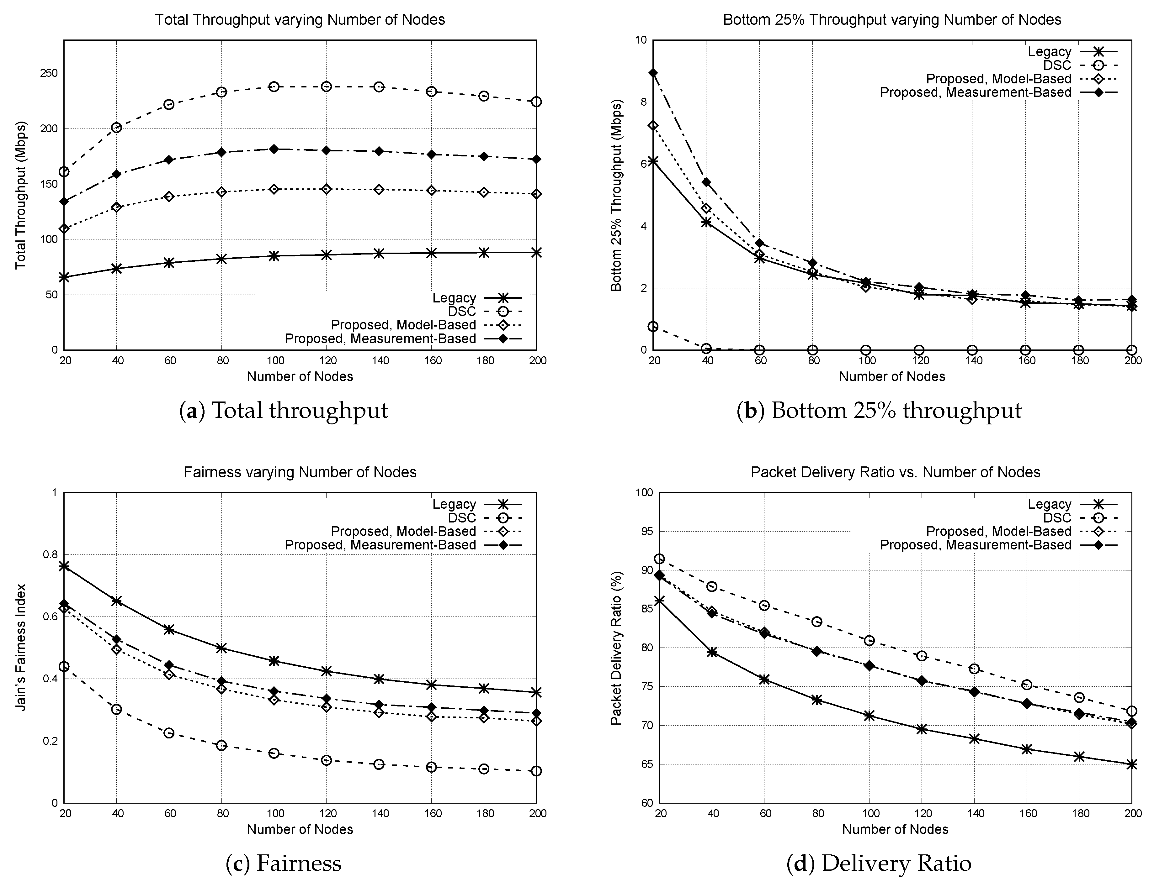
In the first experiment, we have placed 100 APs in the area, and deployed varying number of nodes to study the impact of node density. The number of nodes was varied from 20 to 200. The result is shown in Figure 5.
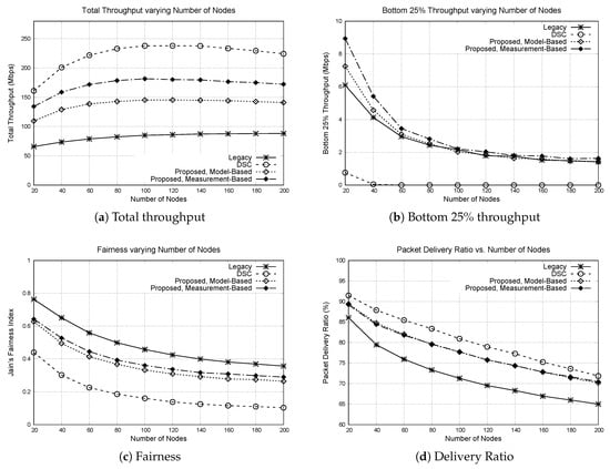
Figure 5.
Performance of protocols varying number of nodes. 100 APs are placed in a grid topology, and 20 to 200 nodes are randomly deployed in the area. (a) total throughput, (b) bottom 25% throughput, (c) Jain’s fairness index, (d) packet delivery ratio.
First of all, the total throughput of all protocols increases with the number of nodes up to a certain point, and then start to decrease. This means that when the number of nodes is small, the space is not fully used and there is room for more concurrent transmissions. However, when the number of nodes becomes large, the space becomes saturated and the throughput degrades due to increased packet collision rate. The increase in packet collisions is reflected in the packet delivery ratio. While the total throughput increases with number of nodes, the bottom 25% throughput rapidly degrades as the number of nodes increase. This means that the channel share becomes less fair, as also can be observed from the fairness graph. With more nodes, the chance of packet collision increases, because the probability that two or more nodes finish the backoff at the same time increases. When two nodes transmit simultaneously, there is higher chance that the packet transmitted from a node closer to the AP survive, compared to the packet transmitted from an edge node. Once an edge node loses packet, it will double its contention window to avoid future collisions, which further reduces the channel share of edge nodes. Thus, more packet collisions lead to lower fairness.
Comparing the protocols, we can observe that DSC achieves the highest total throughput. However, the bottom 25% throughput of DSC is almost zero for most cases. This means that DSC favors small number of mobile nodes that are closely located to their APs. This behavior of DSC is also reflected in the fairness, where DSC shows the lowest fairness index among all protocols. The delivery ratio of DSC is the highest, but it is because transmission of edge nodes is suppressed by the center nodes.
The proposed protocol achieves higher total throughput compared to the legacy 802.11 DCF. More importantly, this total throughput is achieved while maintaining the bottom 25% throughput. For nodes that are close to APs, higher throughput is achieved by setting CST high and aggressively transmitting concurrently with other nodes. Meanwhile, transmissions by the edge nodes are protected by advertised CSTs. Thus, the throughput of the bottom 25% nodes is maintained. In terms of fairness, the proposed protocols achieve lower fairness index compared to the legacy protocol. This is because while the throughput is increased for center nodes, the throughput of the edge nodes remains similar when the proposed protocol is used.
Comparing the model-based and the measurement-based schemes, the measurement-based scheme achieves higher total throughput, and similar bottom 25% throughput compared to the model-based throughput. The model-based chooses the advertised CST by assuming that an interfering node exists at the farthest position from the node, which is a conservative approach. The measurement-based scheme, on the other hand, chooses CST to block the potential interfering node based on RSSI measurement, which could result in higher CST compared to the model-based scheme. Please note that in this experiment and the following experiments, the path loss exponent of the path loss model used in the model-based scheme and the simulation is the same. Later, we study the impact of mismatch in the path loss model.
4.2.2. Varying Number of APs
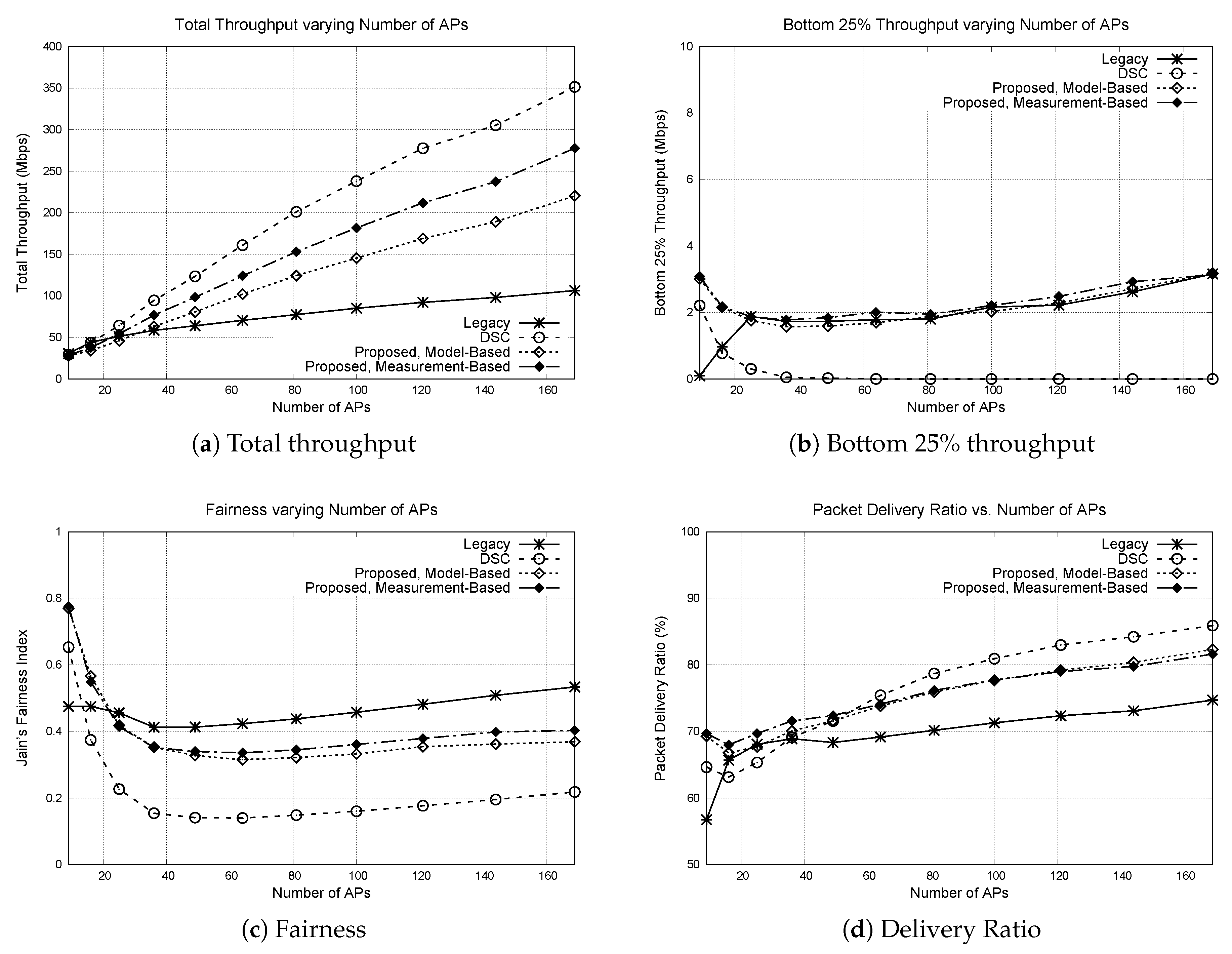
In the second experiment, we have varied the number of APs from 9 to 169. The number of nodes were fixed at 100. When AP density is high, the average distance between a mobile node and its AP becomes shorter. Thus, more concurrent transmissions are expected to take place. The result is shown in Figure 6.
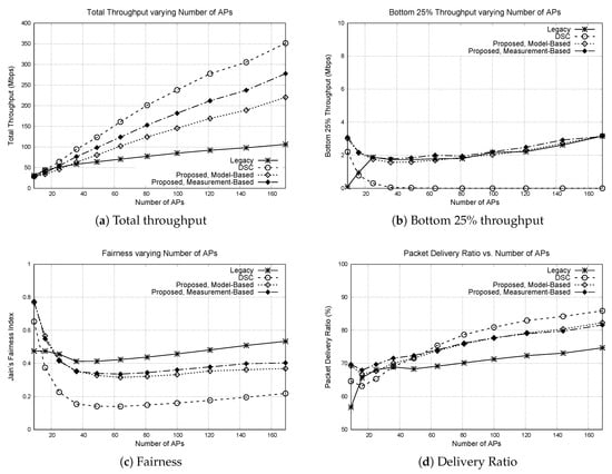
Figure 6.
Performance of protocols varying number of APs. Number of APs is varied from 9 to 169, whereas the number of nodes is fixed to 100. (a) total throughput, (b) bottom 25% throughput, (c) Jain’s fairness index, (d) packet delivery ratio.
First we look at the total throughput. When the number of APs is small, the total throughput is similar for all protocols. However, as the number of APs become large, the difference in throughput also becomes larger. For the legacy 802.11 DCF, the throughput is increased with AP density, but not so much compared to the other protocols. This is because the protocol uses fixed CST. Regardless of whether the mobile node is close to the AP or not, the region that the node blocks while transmitting is the same. Thus, spatial reuse does not improve much even when the average distance between the nodes become small. Still, some throughput increase is observed for the legacy protocol, when the AP density is high. This is because when multiple nodes transmit simultaneously because of random backoff, there is higher chance that the packets will be successfully received by the receivers. DSC achieves the highest total throughput, but causes starvation at the edge nodes as can be observed from the bottom 25% throughput and the fairness. The proposed protocol achieves higher total throughput and comparable bottom 25% throughput, similar to the previous experiment.
For the bottom 25% throughput, the throughput starts to decrease as the number of APs increase, and then after some point starts to increase. A similar trend can be observed in the fairness graph. The reason behind this increase of fairness is due to the increased delivery ratio. Even in the face of packet collisions, the probability that the packets will be successfully received by their receivers increases when the distance between the mobile node and the AP becomes smaller. When the number of APs is very small, possibility of concurrent transmissions is limited because an AP can only transmit to one mobile node at a time. The space is not saturated, and the edge nodes have higher opportunity to send packets. As the number of APs increase, number of concurrent transmissions increases and the fairness is decreased as discussed in the previous experiment. Once the space is saturated, the fairness (and the bottom 25% throughput) starts to increase again due to improved delivery ratio. One peculiar point in the graph is that the performance of legacy 802.11 DCF is very bad when the number of AP is small. This is because some APs at the center of the area are continuously blocked by the fixed CST, when the APs on the edge of the area transmit packets. For example, when the number of APs is 9 (placed in a 3 × 3 grid), the AP at the center rarely gets a chance to transmit, because the APs at the outside take turns to block the AP and prevent it from counting down its backoff counter. Thus, all mobile nodes associated with the AP are starved and the channel share becomes significantly unfair. For other protocols, the center AP may get more opportunity when the other APs transmit, because when the AP on the outside transmits, the required CST could be set high if the mobile node is placed closely to the AP. In that case, the center AP may not be blocked by the transmission, and thus can obtain opportunity to transmit its packet.
4.2.3. Varying Margin
For both the model-based scheme and the measurement-based scheme, a margin parameter is used to account for variations in the channel and the possibility of multiple interfering signals. In the previous simulations, we used 6 dB as the default margin. In this simulation, we study the impact of this margin parameter. In the simulation area, we have placed 100 APs in a grid topology and deployed 100 mobile nodes in random locations. We have varied the margin from 0 dB to 10 dB. The result is shown in Figure 7.
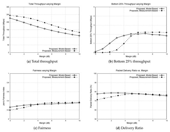
Figure 7.
Performance of the model-based scheme and the measurement-based scheme varying margin. Number of APs and number of nodes are fixed to 100, and the margin is varied from 0 dB to 10 dB. (a) total throughput, (b) bottom 25% throughput, (c) Jain’s fairness index, (d) packet delivery ratio.
Intuitively, the total throughput of the protocols decreases as the margin becomes larger. Larger margin means the CST is lower, which leads to conservative transmissions. Because of that, the bottom 25% throughput increases when the margin becomes larger. For both the model-based and the measurement-based schemes, the bottom 25% throughput increases with the margin up to some point, and then stays similar afterwards. When the margin is lower than the saturation point, the selected CST causes hidden terminals which leads to packet collisions and unfair channel share. For the simulation environment we use, the proper margin to be used for the model-based scheme and the measurement-based scheme is approximately 5 to 6 dB. This is why we used 6 dB as the default margin for other simulations.
From the graphs, we can observe that when the margin becomes low, the measurement-based scheme is affected more significantly compared to the model-based scheme. When the margin is below 6 dB, the bottom 25% throughput significantly drops for the measurement-based scheme, whereas the drop rate is slower for the model-based scheme. The same pattern can be observed for the fairness index and the packet delivery ratio. This is because the measurement-based scheme is more aggressive in setting the CST compared to the model-based scheme. The optimal margin value can be different based on the environmental factors such as node density and AP density. Estimating the potential aggregate interference on the receiver and setting the margin value accordingly is an important and challenging issue, and is left as a future work.
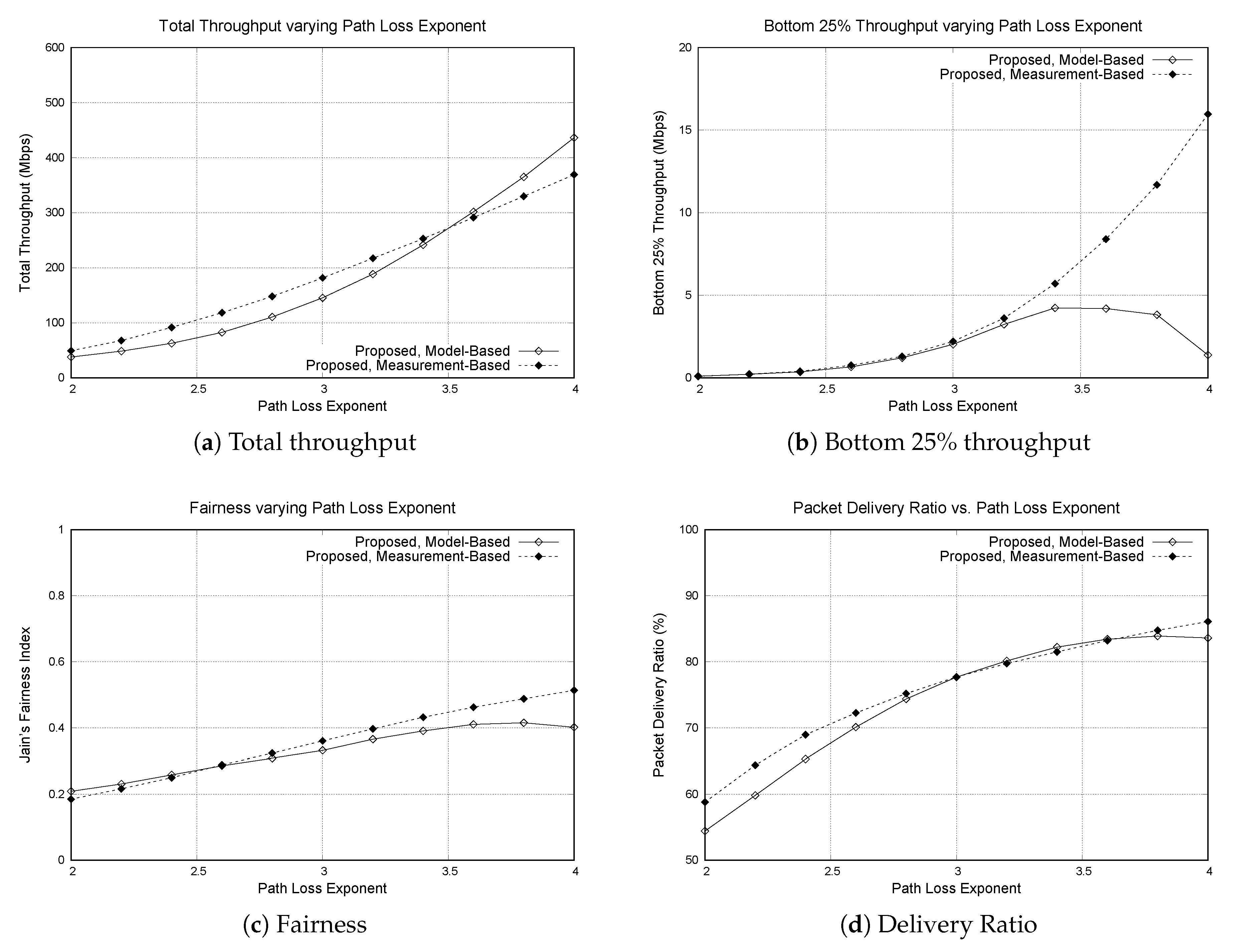
4.2.4. Varying Path Loss Exponent
Until now, the path loss model used in the simulations is identical to the model used in the model-based scheme. The weakness of the model-based scheme is that performance degrades as the gap between model and the real path loss increases. To study its effect, we have varied the path loss exponent in the log-distance model from 2 to 4. The exponent used in the model-based scheme is fixed to 3. Please note that the path loss exponent reflects the propagation characteristics of an environment. For example, empirically obtained path loss exponent for free space, office with soft partition and office with hard partition are 2, 2.6, and 3.0 [25]. Similar to the previous experiment, 100 APs and 100 mobile nodes were placed in the simulation area. The result is in Figure 8.
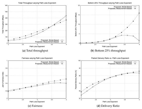
Figure 8.
Performance of the model-based scheme and the measurement-based scheme varying path loss exponent . For the model-based scheme, the mismatch between the model and the real environment can affect the performance. (a) total throughput, (b) bottom 25% throughput, (c) Jain’s fairness index, (d) packet delivery ratio.
As the path loss exponent becomes higher, the total throughput of both model-based and measurement-based protocols increase. With high path loss exponent, the signal strength quickly drops down as the distance is increased. Thus, if the signal source and the interference source is at the same position, the receiver receives the packet with higher SNR if the path loss exponent is higher. When we look at the bottom 25% throughput, the throughput of model-based scheme is degraded when the path loss exponent becomes high, whereas the throughput of measurement-based scheme continuously increases. This means that the model-based scheme is creating hidden terminals. When the path loss exponent of the environment is higher than the model, the CST estimated from the model is higher than the necessary CST to avoid the hidden terminal problem. In other words, the carrier-sense range is set smaller due to the mismatch between the model and the real environment. On the other hand, the measurement-based scheme does not use path loss models to calculate the CST. Thus, it could be a better solution when the path loss condition cannot be precisely modeled.
In summary, the proposed protocol increases system throughput by improving spatial reuse, while not starving the edge nodes. While the model-based scheme is simpler and does not require exchanging neighbor information, it might create hidden terminals if the real path loss is far from the model used to calculate the CST. On the other hand, the measurement-based scheme does not rely on path loss models but uses neighbor information to calculate the CST. As shown in the simulation results, the measurement-based scheme outperforms the model-based scheme especially when the model does not reflect the real environment well. While the measurement-based scheme can be preferred due to its performance and robustness, the model-based scheme could also be practical due to its simplicity such as less requirements for exchange of control messages and data management.
5. Conclusions
In this paper, we have proposed a medium access control protocol for wireless LANs where carrier-sense thresholds are dynamically selected to improve spatial reuse. When a node transmits a packet, it includes a CST value required to protect the transmission in the preamble. A neighboring node considers the advertised CST and its own CST, and transmits concurrently if it finds out that the on-going transmission and its transmission will both be successful. Mobile nodes near the APs can transmit more aggressively because their transmissions can still be received by the receiver in the face of high interference. At the same time, transmissions from edge nodes are protected by the advertised CST. Even if a node can successfully transmit its packet, it defers transmission if it receives a preamble from another node and finds out that its transmission will destroy the on-going transmission. When calculating CST, we have proposed two schemes; the model-based scheme and the measurement-based scheme. In the model-based scheme, each node calculates its own CST assuming the worst-case scenario in which an interfering node exists at the farthest position from the node. Although the scheme does not require any additional control messages, its performance may degrade if the gap between the model and the real environment is large. On the other hand, the measurement-based scheme uses neighbor information exchanged between the nodes to calculate the CST. The simulation results show that the proposed protocol achieves high throughput while protecting the channel share of the edge nodes. Currently, the CST calculation is based on a single interfering node, and multiple interfering nodes are accounted for using the margin parameter. The margin parameter is also used to address channel variations and possible existence of external interference. However, the fixed margin value could fail to cover these factors and may lead to either too conservative transmissions degrading spatial reuse, or too aggressive transmissions creating hidden terminals and degrading fairness of the system. As discussed in the paper, it could be better to have nodes independently select the margin based on their conditions such as density of neighbors and variation of measured RSSIs. Calculating proper margin based on the environment is a challenging issue and is a subject for future work. More accurate estimation of aggregate interference is another topic for future work, as it will lead to a better calculation of CSTs.
Author Contributions
Conceptualization, J.S., methodology, J.S. and J.L., validation, J.S. and J.L., writing—original draft preparation, J.S.
Funding
This work was supported in part by the National Research Foundation (NRF) of Korea under grant no. 2019R1A2C1005881.
Conflicts of Interest
The authors declare no conflict of interest.
Abbreviations
The following abbreviations are used in this manuscript:
| AP | Access Point |
| BSS | Basic Service Set |
| CA | Collision Avoidance |
| CSMA | Carrier-Sense Multiple Access |
| CST | Carrier-Sense Threshold |
| DCF | Distributed Coordination Function |
| DSC | Dynamic Sensitivity Control |
| MCS | Modulation and Coding Scheme |
| RSSI | Received Signal Strength Indicator |
| SNR | Signal-To-Noise Ratio |
| SR | Spatial Reuse |
| WLAN | Wireless Local Area Networks |
| WMA | Weighted Moving Average |
References
- Bellata, B. IEEE 802.11ax: High-Efficiency WLANs. IEEE Wirel. Commun. 2016, 23, 38–46. [Google Scholar] [CrossRef]
- Selinis, I.; Filo, M.; Vahid, S.; Rodriguez, J.; Tafazolli, R. Evaluation of the DSC algorithm and the BSS color scheme in dense cellular-like IEEE 802.11ax deployments. In Proceedings of the 2016 IEEE 27th Annual International Symposium on Personal, Indoor, and Mobile Radio Communications (PIMRC), Valencia, Spain, 4–8 September 2016. [Google Scholar]
- Yang, X.; Vaidya, N. On physical carrier sensing in wireless ad hoc networks. In Proceedings of the IEEE 24th Annual Joint Conference of the IEEE Computer and Communications Societies, Miami, FL, USA, 13–17 March 2005. [Google Scholar]
- Zhu, J.; Guo, X.; Yang, L.; Conner, W. Adaptive physical carrier sensing to maximize spatial reuse in 802.11 mesh networks. Wiley J. Wirel. Commun. Mob. Comput. 2004, 4, 933–946. [Google Scholar] [CrossRef]
- Zhang, X.; Zhu, H.; Qiu, G. Optimal physical carrier sensing to defend against exposed terminal problem in wireless ad hoc networks. In Proceedings of the 2014 23rd International Conference on Computer Communication and Networks (ICCCN), Shanghai, China, 4–7 August 2014. [Google Scholar]
- Vutukuru, M.; Jamieson, K.; Balakrishnan, H. Harnessing Exposed Terminals in Wireless Networks; USENIX NSDI: San Francisco, CA, USA, 2008. [Google Scholar]
- Chakraborty, S.; Nandi, S.; Chattopadhyay, S. Alleviating hidden and exposed nodes in high-throughput wireless mesh networks. IEEE Trans. Wirel. Commun. (TWC) 2016, 15, 928–937. [Google Scholar] [CrossRef]
- Hosseinabadi, G.; Vaidya, N. Concurrent-MAC: Increasing concurrent transmissions in dense wireless LANs. In Proceedings of the International Conference on Computing, Networking and Communications (ICNC), Kauai, HI, USA, 15–18 February 2016. [Google Scholar]
- Shin, K.; Park, L.; Hong, J.; Har, D.; Cho, D. Per-node throughput enhancement in Wi-Fi densenets. IEEE Commun. Mag. 2015, 53, 118–125. [Google Scholar] [CrossRef]
- Tayamon, S.; Wikstrom, G.; Moreno, K.; Soder, J.; Wang, Y.; Mestanov, F. Analysis of the potential for increased spectral reuse in wireless LAN. In Proceedings of the 2015 IEEE 26th Annual International Symposium on Personal, Indoor, and Mobile Radio Communications (PIMRC), Hong Kong, China, 30 August–2 September 2015. [Google Scholar]
- Kulkarni, P.; Cao, F. Taming the densification challenge in next generation wireless LANs: An investigation into the use of dynamic sensitivity control. In Proceedings of the 2015 IEEE 11th International Conference on Wireless and Mobile Computing, Networking and Communications (WiMob), Abu Dhabi, UAE, 19–21 October 2015. [Google Scholar]
- Mvulla, J.; Park, E.; Adnan, M.; Son, J. Analysis of asymmetric hidden node problem in IEEE 802.11ax heterogeneous WLANs. In Proceedings of the 2015 International Conference on Information and Communication Technology Convergence (ICTC), Jeju, Korea, 28–30 October 2015. [Google Scholar]
- Zhong, Z.; Cao, F.; Kulkarni, P.; Fan, Z. Promise and perils of dynamic sensitivity control in IEEE 802.11ax WLANs. In Proceedings of the 2016 International Symposium on Wireless Communication Systems (ISWCS), Poznan, Poland, 20–23 September 2016. [Google Scholar]
- Ropitault, T. Evaluation of RTOT algorithm: A first implementation of OBSS_PD-based SR method for IEEE 802.11ax. In Proceedings of the 2018 15th IEEE Annual Consumer Communications & Networking Conference (CCNC), Las Vegas, NV, USA, 12–15 January 2018. [Google Scholar]
- Afaqui, M.; Garcia-Villegas, E.; Lopez-Aguilera, E. Dynamic sensitivity control algorithm leveraging adaptive RTS/CTS for IEEE 802.11ax. In Proceedings of the 2016 IEEE Wireless Communications and Networking Conference, Doha, Qatar, 3–6 April 2016. [Google Scholar]
- Murakami, K.; Ito, T.; Ishihara, S. Improving the spatial reuse of IEEE 802.11 WLAN by adaptive carrier sense threshold of access points based on node positions. In Proceedings of the 8th International Conference on Mobile Computing and Ubiquitous Networking (ICMU), Hakodate, Japan, 20–22 January 2015. [Google Scholar]
- Ropitault, T.; Golmie, N. ETP algorithm: Increasing spatial reuse in wireless LANs dense environment using ETX. In Proceedings of the 2017 IEEE 28th Annual International Symposium on Personal, Indoor, and Mobile Radio Communications (PIMRC), Montreal, QC, Canada, 8–13 October 2017. [Google Scholar]
- Selinis, I.; Katsaros, K.; Vahid, S.; Tafazolli, R. Control OBSS/PD sensitivity threshold for IEEE 802.11ax BSS color. In Proceedings of the 2018 IEEE 29th Annual International Symposium on Personal, Indoor and Mobile Radio Communications (PIMRC), Bologna, Italy, 9–12 September 2018. [Google Scholar]
- Huang, C.; Lea, C.-T.; Wong, A. A joing solution for hidden and exposed terminal problems in CSMA/CA wireless networks. Elsevier Comput. Netw. 2012, 56, 3261–3273. [Google Scholar] [CrossRef]
- Huang, J.; Xing, G.; Zhou, G. Unleashing exposed terminals in enterprise WLANs: A rate adaptation approach. In Proceedings of the IEEE INFOCOM 2014–IEEE Conference on Computer Communications, Toronto, ON, Canada, 27 April–2 May 2014. [Google Scholar]
- Adere, K.; Murthy, G.R. Solving the hidden and exposed terminal problems using directional antenna based MAC protocol for wireless sensor networks. In Proceedings of the International Conference on Wireless and Optical Communication Networks (WOCN), Colombo, Sri Lanka, 6–8 September 2010. [Google Scholar]
- Wang, L.; Wu, K.; Hamdi, M. Combating hidden and exposed terminal problems in wireless networks. IEEE Trans. Wirel. Commun. (TWC) 2012, 11, 4204–4213. [Google Scholar] [CrossRef]
- Henderson, T.; Lacage, M.; Riley, G. Network simulations with the ns-3 simulator. Sigcomm Demonstr. 2008, 14, 527. [Google Scholar]
- Jain, R.; Chiu, D.; Hawe, W. A Quantitative Measure of Fairness and Discrimination for Resource Allocation in Shared Computer Systems; DEC Research Report TR-301; Digital Equipment Corporation: Maynard, MA, USA, 1984. [Google Scholar]
- Rappaport, T.S. Wireless Communications Principles and Practices; Prentice-Hall: Englewood Cliffs, NJ, USA, 2002. [Google Scholar]

© 2019 by the authors. Licensee MDPI, Basel, Switzerland. This article is an open access article distributed under the terms and conditions of the Creative Commons Attribution (CC BY) license (http://creativecommons.org/licenses/by/4.0/).