Featured Application
This work provides an effective analysis tool for OCT-based brain imaging and provides an approach to improve the quantitative accuracy of chromophores in tissue for the experimental study of brain functional sensing. What is more, these methods are also suitable for other complex 3D bio-tissues.
Abstract
Optical coherence tomography (OCT) can obtain high-resolution three-dimensional (3D) structural images of biological tissues, and spectroscopic OCT, which is one of the functional extensions of OCT, can also quantify chromophores of tissues. Due to its unique features, OCT has been increasingly used for brain imaging. To support the development of the simulation and analysis tools on which OCT-based brain imaging depends, a model of mesh-based Monte Carlo for OCT (MMC-OCT) is presented in this work to study OCT signals reflecting the structural and functional activities of brain tissue. In addition, an approach to improve the quantitative accuracy of chromophores in tissue is proposed and validated by MMC-OCT simulations. Specifically, the OCT-based brain structural imaging was first simulated to illustrate and validate the MMC-OCT strategy. We then focused on the influences of different wavelengths on the measurement of hemoglobin concentration C, oxygen saturation Y, and scattering coefficient S in brain tissue. Finally, it is proposed and verified here that the measurement accuracy of C, Y, and S can be improved by selecting appropriate wavelengths for calculation, which contributes to the experimental study of brain functional sensing.
1. Introduction
Applications of optical coherence tomography (OCT) in brain tissue include structural imaging and functional sensing. Structural imaging includes macroscopic imaging [1,2] and angiography of the brain tissue [3]. Common detectable brain functional activities are shown in Figure 1 [4,5], and the associated optical processes are also indicated. Among them, scattering and absorption can be obtained by spectroscopic OCT [6,7], and Doppler shift can be measured by Doppler OCT [8]. This paper focuses on the applications of OCT in brain structural imaging as well as in the measurement of absorption and scattering coefficients of brain tissue.
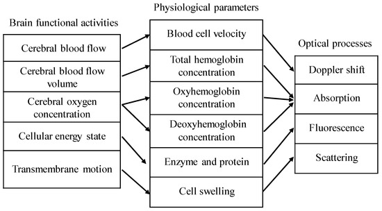
Figure 1.
Relationship among common brain functional activities, physiological parameters, and optical processes. The total hemoglobin concentration C is equal to the sum of the oxyhemoglobin concentration and deoxyhemoglobin concentration. Oxygen saturation Y is the ratio of the oxyhemoglobin concentration to the total hemoglobin concentration.
Both numerical and in vivo testbeds are useful for brain tissue imaging. In vivo testbeds provide the ultimate confirmation of performance, while numerical testbeds allow a more controlled evaluation of imaging modalities and optimization of their parameters. Monte Carlo (MC) simulation is the golden means to simulate the interaction between light and tissue [9,10]. Many efficient MC models have been developed to study OCT signals of different tissues [11,12,13,14] or polarization-sensitive OCT [11,15]. However, there are few literatures to analyze OCT signals in brain tissue using MC technology. Therefore, as a slight supplement to this field, we detail how to use MC simulation to analyze the applications of OCT in brain tissue structural imaging and functional sensing. A model of mesh-based Monte Carlo [14,16,17] for OCT (MMC-OCT) is used in this paper, which is useful for any complex three-dimensional (3D) bio-tissues. This work provides an analysis method and related data for brain simulation as well as help for experimental study.
Quantitative accuracy is undoubtedly an important indicator in the measurement of scattering and absorption of brain tissue. In the spectroscopic OCT, extinction coefficients of different wavelengths are obtained by using the short-time Fourier transform (STFT) and exponential fitting [7], and the extinction coefficient is the sum of the absorption coefficient and scattering coefficient S. It is a common choice to use a visible light waveband for detection of scattering and absorption [6,18], and the main absorption in this range comes from hemoglobin for brain tissue [19,20]. Thus, the total hemoglobin concentration C and oxygen saturation Y of the brain tissue can be calculated by solving linear equations using absorption coefficients of several different wavelengths [4], where C and Y are defined in Figure 1. The extinction coefficients of multiple wavelengths can be obtained in spectroscopic OCT, so the results obtained by fitting the oversampled data will undoubtedly be more accurate considering the noise and experimental errors in the actual applications. However, the spectral resolution and spatial resolution are contradictory [21], and the more positions the window function traverses, the longer the calculation time. In addition, the narrower the width of the window function in the spectral domain, the worse the signal-to-noise ratio (SNR). For measurements of blood vessels with high hemoglobin concentrations (~2 mmol) [22], two or three wavelengths can be used to resolve the correct functional parameters [23,24] while achieving high spatial resolution. In the process of solving C, Y, and S from the fitted extinction coefficients of three wavelengths, we found that the error of the extinction coefficient has a great influence on the calculated results, and the values of C, Y, and S calculated using different wavelengths are distinct for the certain error. Therefore, the selection of wavelengths that are used to calculate scattering and absorption is explored in this paper. It is proposed and validated here that the measurement accuracy of C, Y, and S can be improved by selecting the appropriate wavelengths for calculation.
The remainder of this paper is organized as follows. We present the basic principles of structural imaging and functional sensing of OCT as well as MMC-OCT models in Section 2. In Section 3, we first detail how to use MMC-OCT simulation to study structural imaging of tissue, and then the influences of different wavelengths on quantitative accuracy of scattering and absorption coefficients are discussed. Finally, in Section 4 we provide a brief summary and conclusion.
2. Methods
2.1. Structural and Functional Imaging Based on OCT
The spectroscopic OCT includes the spectroscopic time domain OCT (TD-OCT) and spectroscopic Fourier domain OCT (FD-OCT), both of which are implemented by windowed Fourier transform [21,25]. Here we mainly introduce the principle of structural imaging and functional sensing based on FD-OCT. In FD-OCT, it is only necessary to perform a Fourier transform on the interference signal collected by the spectrometer or detectors to obtain the structural image, i.e.,
and
where S(k) is the power spectrum of the light source; aR is the amplitude of the reflected reference light; k is the wavenumber; n(k) is the refractive index of the sample at k; and a(z) is the amplitude of the backscattered light at the z position of the sample. AC represents the self-coherent signal of the sample, which can usually be ignored because it is small.
During the calculation above, n(k) is treated as a real number. However, it is in fact a complex valued function , defining both the group delay (n(k)) and absorption () within a medium [26]. Therefore, ignoring the conjugate and direct-current terms, Equation (2) should be expressed as
in which μt is the extinction coefficient of tissue; and n is the average refractive index of tissue. When a STFT or wavelet transform is applied to Equation (1), we can obtain the depth-resolved spectrum H (z, kn), shown as
where A represents the system parameter and μb is the backscattered coefficient [7] and is a window function having a width Δk centered at a mean scattering wave number . Thus, the spectra of backscattering coefficient μb and extinction coefficient μt as a function of z and are obtained.
From Equation (4) we can see that there is an inherent trade-off between spectral resolution and spatial resolution. For Gaussian windows, the resolution in z-space and k-space is related by Equation , i.e., [21].
For brain tissue, the main absorption comes from water and hemoglobin. For simplicity, chromophores other than hemoglobin such as fat, melanin, and lipids are neglected [19]. Consequently, the extinction coefficient of the sample can be defined as
εO and εD are the molar extinction coefficients—the extinction coefficient divided by ln(10) per unit molar concentration—of oxyhemoglobin and deoxyhemoglobin, respectively [27]. μs is the scattering coefficient. The unit of C is mmol, the unit of εO and εD is mmol−1 mm−1, and the unit of μs and μt is mm−1. Functional sensing involves the measurement of C, Y, and μs based on the absorption and scattering spectra (Figure 2). Figure 2 shows the curves of μa and μs as a function of wavelength, where and C = 2 mmol [22].
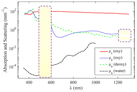
Figure 2.
Wavelength dependence of oxyhemoglobin and deoxyhemoglobin absorption (blue and green, respectively) [22], whole blood scattering (red) [22], and water absorption (black) [20].
For the visible-light waveband (500–600 nm), the magnitude of the absorption and scattering coefficients are of the same order, and it can be approximately considered that the scattering coefficient is not affected by the wavelength when using the method introduced in [6]. Therefore, the extinction coefficient can be expressed as
Consequently, it is only necessary to obtain the extinction coefficients of three different wavelengths at a certain depth z, and then, C, Y, and μs can be calculated by solving the ternary equation.
In the near-infrared light waveband (600–1100 nm), the scattering coefficient is affected more by the wavelength than in the visible range, and the scattering coefficient is approximately linear with the wavelength or satisfies a specific functional relationship a × λb [28,29], where both a and b are constants. Therefore, the extinction coefficient can be expressed as
when the linear relationship is considered. Accordingly, C, Y, and μs can be calculated by solving the quaternary equation.
In the range of >1200 nm, the absorption coefficients of oxyhemoglobin and deoxyhemoglobin are almost indistinguishable as shown by the purple dashed box in Figure 2, so the functional sensing is difficult to achieve.
This article focuses on functional sensing in the visible-light waveband. Within this range, the parameter C, Y, and S can be obtained by solving a ternary linear equation, expressed as Equation (6), or can be obtained by the fitting strategy using oversampled data. The latter has a higher probability of getting the correct parameters. However, if functional parameters with acceptable errors can be obtained using data at three wavelengths, it is advantageous where high spatial resolution is required, such as imaging small-sized microvessels in brain tissue.
2.2. Mesh-Based Monte Carlo for Optical Coherence Tomography (MMC-OCT)
Throughout the simulation of this paper, a fast mesh-based Monte Carlo (MMC) photon migration algorithm for imaging in 3D complex tissue was used [16,17], and a schematic that clearly illustrates the simulation process is shown in Figure 3. Before proceeding with the steps described in Figure 3, the “MMCLAB” package needs to be downloaded [30], which contains all the MATLAB m-files mentioned in Figure 3.
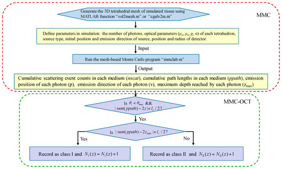
Figure 3.
Flow chart describing the simulation process of mesh-based Monte Carlo optical coherence tomography (MMC-OCT). μa and g are the absorption coefficient and anisotropy factor, respectively; is the angle between the emission direction of the detected photon and z axis; is the collecting angle; lc is axial resolution (i.e., the coherence length); z is the probing depth; sum (nscat) and sum (ppath) represent the sum of scattering events and the sum of path lengths in all media, respectively. NI (z) and NII (z) are the numbers of class I photon and class II photon that are reflected/backscattered at the z-depth, respectively.
In simulations, the light source was a pencil beam, and a circular detector with a radius of 10 μm was placed at the same position as the emission position of the photon packet. The initial set number of photons and were 5 × 10¹³ and 3°, respectively. After running Monte Carlo MATLAB program “mmclab”, the parameters nscat, ppath, v, and zmax of each detected photon are obtained. It should be noted that the mesh of the tissue is subdivided in the depth direction in order to obtain the depth coordinates at which the scattering event occurs. Then, according to the condition , the photons within the collecting angle are divided into different depths z having a thickness of lc. To classify the photon further, on satisfaction of , the photon is recorded as a class I photon, otherwise it is recorded as a class II photon [10,13].
We directly obtained the backscattered field of the tissue detected by the OCT system represented as Equation (3) through the above steps, without simulating the complete imaging process of the OCT. The resolution of z-space is equal to lc, which is determined by the spectral bandwidth of the light source, and μt is the average extinction coefficients of the tissue within the spectral bandwidth.
Similarly, for the analysis of functional imaging of FD-OCT, the depth-resolved spectrum H (z, kn) represented by Equation (4) was directly obtained. From Equation (4), we found that the effect of window function g in the STFT is equivalent to that of a light source with a narrower spectral width. Therefore, we controlled the z-space resolution by setting lc, and the expression of lc is [21]. μt is the extinction coefficient of the tissue over the spectral bandwidth of the window function.
All simulations were run using a desktop computer with an Intel Core 3-GHz 64-bit processor (Intel Corporation, Santa Clara, CA, USA) and 16 GB of RAM running the Windows operating system. It, however, has to be pointed out that the simulation time of MMC-OCT is long. Simulation of a 300 × 300 × 500 μm gray matter (discretized using a mesh of 15,720 nodes and 87,996 elements) for 5 × 10¹¹ photons took approximately 2.5 h per A-scan. However, the simulation time can be greatly reduced by improving the program. It has been proven that tetrahedral mesh-based MC and importance sampling can significantly reduce computation time, which can obtain more accurate OCT signals using fewer photons [31]. In addition, because of the inherently parallel nature of MC simulation, we can reduce simulation time by implementing the MMC-OCT program on a graphics processor unit (GPU).
3. Results and Discussions
We first generated a segmented human brain atlas as shown in Figure 4 [32], from which we know that the brain tissue has a hierarchical structure and some cylindrical structures (vessels) embedded in it.
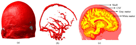
Figure 4.
Three-dimensional (3D) brain atlas (181 × 217 × 181 mm): (a) 3D model of brain; (b) 3D model of blood vessels segmented from brain model shown in (a); and (c) 2D section of brain extracted at plane x = 90 mm. CSF represents the cerebrospinal fluid.
3.1. Simulation Results of Brain Structural Imaging
In this section, the structural imaging of hierarchies and vascular structures present in the brain tissue was simulated. The parameters of the hierarchical structure [16,33] and vessel structure [22] in the simulation are listed in Table 1. The n and g of tissue were 1.37 and 0.9, respectively. The simulated hierarchy structure consisted of the skull, cerebrospinal fluid (CSF), gray matter and white matter, and its 3D volumetric finite-element (FE) mesh is shown in Figure 5a. Figure 5b shows the 3D volumetric mesh of gray matter with a blood vessel embedded in it, and the position of the blood vessel is indicated on the figure. The numbers in Figure 5a,b represent the number of grids, and the grid resolution was 10 μm. In the simulation, the center wavelength was 630 nm and lc was 10 μm, which is equivalent to using a light source having a spectral bandwidth of 13 nm.

Table 1.
Geometric parameters and optical parameters of simulated tissues at 630 nm wavelength.
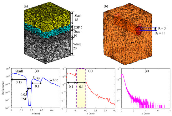
Figure 5.
(a,b) 3D volumetric finite-element (FE) mesh of simulated tissue, in which R and O are the radius and center of the blood vessel, respectively. (d) Backscattered signal of the vessel tissue. (c,e) show the backscattered signal of the compressed and uncompressed hierarchical structures, respectively.
First, in order to verify the correctness and effectiveness of the MMC-OCT model in OCT-based structural imaging, all parts of the hierarchy structure were compressed, and compressed sizes are shown inside parentheses in the “Thickness” column of Table 1. The backscattered signal of the compressed hierarchical structure (Figure 5c,d) shows the simulation result of the vessel structure obtained with actual tissue parameters. It is clearly seen that the backscattered signals reflect the structural distribution of the two tissues, and the dimensions of each part are identical to the preset structural dimensions. Moreover, the results show that the larger the scattering coefficient, the larger the amplitude of the backscattered signal and the faster the signal attenuates, which is completely consistent with the actual situation [7] and proves the validity of the MMC-OCT used in this paper.
Figure 5e shows the simulation result of the brain hierarchy structure obtained using actual tissue parameters shown outside parentheses in the “Thickness” column of Table 1. It can be found that the backscattered signal attenuates rapidly with an increase in depth and the light cannot penetrate the skull, which is consistent with reality [4]. The imaging depth of SD-OCT is generally 1–2 mm, owing to the large attenuation coefficient of tissue, which is not enough for human brain tissue [4]. But for some in vitro studies, we may only focus on a part of the brain, such as the cerebral cortex or the vascular network. In addition, brain imaging of small animals also provides significant reference value for human brain research. In the aforementioned applications, the MMC-OCT can be used to simulate their imaging process, thus providing important theoretical support for brain imaging.
3.2. Simulation Results of Brain Functional Sensing
As we mentioned in the introduction, the application of spectroscopic OCT in brain functional sensing is usually to quantify three parameters: total hemoglobin concentration C, blood oxygen saturation Y, and scattering coefficient S. After obtaining the OCT signals of different wavelengths using MMC-OCT, C, Y, and S can be calculated using the quantitative method introduced in Section 2.1. In this section, we studied brain functional sensing through theoretical analysis and MMC-OCT simulation. Specifically, we explored factors that affect the quantitative accuracy of C, Y, and S using three wavelengths.
In the visible light waveband (500–600 nm), the absorption coefficient of hemoglobin is much larger than that in the near-infrared waveband, as shown in Figure 2, so functional sensing is very advantageous. Therefore, we chose a visible waveband to simulate functional sensing of the brain tissue. To obtain parameters C, Y, and S, we usually need to solve the following three-variable linear equations:
in which subscripts 1, 2, and 3 represent three different wavelengths. ln(10) is multiplied to εO and εD. The extinction coefficients μt1, μt2, and μt3 that are obtained by exponential fitting of the backscattered signals include the experimental error and data fitting error. The solutions to Equation (8) are
and
where , and the parameters with (′) as a superscript are the results of subtracting the corresponding parameters of the second wavelength from the parameters of the third wavelength. The variation of the three parameters C, Y, and S caused by the errors of μti (i = 1, 2, and 3) can be expressed as
and
in which , , and all represent errors of μti, and their signs and magnitudes are uncertain in practice.
It can be seen from Equations (12)–(14) that the calculation errors of C and S have nothing to do with Y and are only related to the errors of μti and the absorption parameters of the selected wavelengths. However, the calculation error of Y varies with μti, that is, it is related to C, Y, and S. In addition, we find that the change trends of |dC| and |dS| are the same, while that of |dY| is opposite to the other two. In other words, we have no way to choose the optimal three wavelengths to minimize the errors of the C, Y, and S simultaneously, but can only make compromises according to the actual situation. For example, if the requirement for the accuracy of C is higher in practical application, the denominator of |dC| can be larger and the numerator smaller by choosing appropriate wavelengths, while if the requirement for the accuracy of Y is higher, the opposite choice can be made.
Figure 6 shows the errors of C, Y and, S under two different wavelength choices, and the corresponding absorption parameters are shown in the pictures. It should be noted that these parameters are not actual values shown in Figure 2, but are obvious cases set to explain the above rules. In the simulation, C was 100 μM, Y was 70%, and S was 7 mm−1. The C of the brain tissue is approximately 100 μM [19]. Here, for convenience, we assumed that μt1 had error dμt1, and μt2 and μt3 had no errors. In Figure 6a, when dμt1 is 0.1 mm−1, dC/C = 0 and dS/S = 0.028, while dY/Y is up to 0.9. In Figure 6b, when dμt1 is 0.1 mm−1, dC/C = 3.3 and dS/S = 1.16, while dY/Y is only 0.2. Therefore, we can choose the appropriate wavelengths to solve the scattering and absorption parameters according to the actual needs.
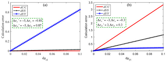
Figure 6.
Calculation errors of three parameters when dC is small (a) and when dY is small (b).
Next, functional sensing of brain tissue was simulated using MMC-OCT. The most popular components of brain tissue for researchers are often the cerebral cortex (i.e., gray matter) and blood vessels, so we obtained backscattered signals at different wavelengths of vascular tissue. The blood vessel had a diameter of 50 μm and was embedded in the gray matter tissue with a depth of 150 μm. Firstly, the appropriate wavelengths were selected based on the spectral data shown in Figure 2. We set a light source with a center wavelength of 570 nm and a spectral width of 50 nm. The window function of the STFT has a width in the spectral domain of 15 nm, and there is no overlap between the window functions at the two adjacent wavelengths. Between 540 nm and 600 nm, we used Equations (12)–(14) to calculate the theoretical error of the three parameters obtained using different wavelength combinations, and each combination consists of three wavelengths with an interval of 15 nm. The error for each μt is a random number within 0–0.1 mm−1; Y = 0.7, C = 2 mmol, and S = 70 mm−1. The curve in Figure 7a shows the sum of the errors of the three parameters calculated using different wavelength combinations, and the abscissa is the minimum of the three wavelengths. The number of calculations is 200.
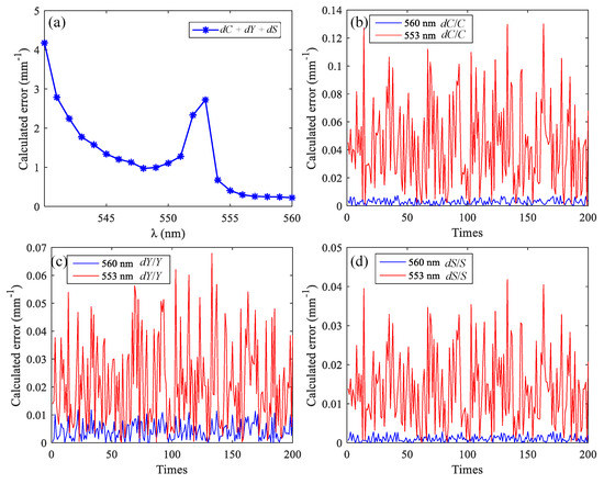
Figure 7.
(a) The sum of the errors of the three parameters calculated using different wavelength combinations; calculation errors of C (b), Y (c), and S (d) calculated using the optimal wavelength combination and the worst wavelength combination.
Within the spectral bandwidth of the source, the optimal and worst combinations are 560 nm, 575 nm, 590 nm and 553 nm, 568 nm, 583 nm, respectively. Figure 7a–c shows the calculation errors of C, Y, and S, respectively. Since the error of the extinction coefficient is random, we compare the maximum of the 200 calculation errors of the two combinations. The maximum values of the dC/C, dY/Y, and dS/S of the optimal combination are reduced by 17.6, 5.8, and 14.5 times, respectively, compared to those of the worst combination. The optical parameters of the two combinations are shown in Table 2, and Figure 8 shows the simulation results using MMC-OCT. When using the method described in [6], it can be approximated that the scattering coefficient is not affected by the wavelength, so we set the scattering coefficient for each wavelength to 70 mm−1.
Table 2.
Optical parameters of optimal and worst wavelength combinations for functional sensing.
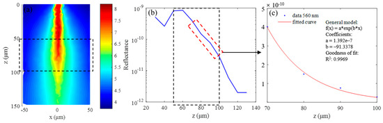
Figure 8.
Simulation results for 560 nm wavelength: (a) continuous wave (CW) fluence extracted at plane y = 0 μm; (b) backscattered signals; and (c) fitting results when class II photons are removed.
The simulation results for the 560 nm wavelength are summarized in Figure 8. Figure 8a shows the continuous wave (CW) fluence extracted at plane y = 0 μm, and the black dotted box in the figure indicates the position of the blood vessel. The blue curve in Figure 8b is the backscattered signal, and the signal in the depth range of 70 μm–100 μm is selected to calculate the extinction coefficient by exponential fitting, the results of which are shown in Figure 8c. The fitting coefficients and goodness are shown in the picture, and the R2 value of the fitting results is 0.9969. The fitting results of two combinations and C, Y, and S calculated from the fitting results are listed in Table 3. The parameters marked “The” in Table 3 are the theoretical calculation values, and those labeled “Rea” are the simulation values. It can be seen that the two are basically the same, and the maximum error is 0.06 mm−1. Of course, this does not mean that the error in the actual experiment is also at this level, but rather illustrates the feasibility of the MMC-OCT in simulating the process of obtaining the extinction coefficient.
Table 3.
Fitting results and calculated C, Y, and S for two combinations.
The errors of C, Y, and S obtained by the optimized combination of wavelengths are much smaller than those obtained by the worst combination, and the calculation errors of C, Y, and S are reduced by 160, 16.75, and 238.8 times, respectively.
The results in Table 3 show that we can obtain very accurate optical parameters of blood vessels by reasonably selecting three wavelengths. However, the error between the theorical extinction coefficient and the simulation result is very small, not exceeding 0.06 mm−1, so the result is ideal. In actual experiments, when the method described in [34] is used, the accuracy of the exponentially fitted extinction coefficient can reach 0.8%, which is about 0.72 mm−1 for blood. Therefore, we set the maximum error of extinction coefficient to 1 mm−1. At Y = 70%, dC/C, dY/Y, and dS/S calculated by the optimized combination are 0.0859, 0.0829, and 0.0296, respectively. Accordingly, we can conclude that when imaging vascular structure, the optimization scheme shown in Figure 7 can be used to reasonably select three wavelengths to calculate the optical parameters of the tissue while ensuring high spatial resolution.
It should be noted that the above optimization process was performed under the condition that Y = 0.7. The hemoglobin concentration of the blood vessel is high, and the absorption coefficient in the visible-light waveband is large, so the optimization results for different Y are approximately the same.
Next, the functional sensing of the cerebral cortex was discussed, where the spatial resolution requirements are reduced compared to imaging small-sized blood vessels. In the simulation, wavelengths of 540 nm, 546 nm, and 576 nm were selected, and the window function of the STFT has a width of 6 nm in the spectral domain. Optical parameters of gray matter at these wavelengths are listed in Table 4. There were two reasons for this choice. First, the scattering coefficients of these three wavelengths were approximately the same, as shown in Figure 2; second, we made a compromise by considering the calculation errors of C and Y. It should be noted that this selection of wavelengths was obtained under the condition that Y = 70% using the optimization method described in Figure 7. The n and g of tissue were 1.37 and 0.9, respectively. The scattering coefficients S in the Table 4 were obtained by dividing the scattering coefficients in Figure 2 by 10 so that they were approximately the same as the scattering coefficients in gray matter [35].
Table 4.
Optical parameters of gray matter at selected wavelengths for functional sensing.
The simulated gray matter was a 300 × 300 × 500 (μm) cube, and simulation results are shown in Figure 9. Figure 9a shows the CW fluence extracted at plane y = 0 μm. The black data points in Figure 9b represent backscattered signals, and the interval of z is 25 μm. The green curve in Figure 9b is the fitting result, and the fitting coefficients and goodness are shown in the picture. The R2 value of the fitting results is 0.9908. The fitting result in Figure 9b was obtained after removing the class II photons. If class II photons are not removed, the fitting μt is small, as shown in Figure 9c because the optical path of the class II photon is larger. For comparison, the data in Figure 9c were normalized. The theoretical calculation values and simulation values of the three parameters are shown in Figure 9d. The points marked “The” in the legend are the theoretical calculation values, and the points labeled “Rea” are the simulation values.
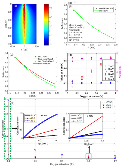
Figure 9.
Simulation results in visible waveband: (a) CW fluence extracted at plane y = 0 μm; (b) backscattered signals and fitting results; (c) fitting results when class II photons are removed and when class II photons are not removed; (d) theoretical calculation values and simulation values of C, Y, and S; and (e) differences between theoretical calculation values and simulation values.
It can be seen from Figure 9d that the simulation values are basically in accordance with the theoretical calculation values except that the deviation of Y at Y = 10% is a little large, which is because the calculation error of Y varies with the value of μt, as described in Equation (13). The results of Figure 9e are the differences between the theoretical calculation values and simulation values. The pre-estimated calculation errors in the case that Y = 10% and Y = 70% are shown in Figure 9e, which can be seen to be consistent with the results of the actual simulation. If we predict that the Y of tissues is relatively high, then the choice of wavelengths is reasonable now. On the contrary, the current wavelengths selection is unreasonable if we predict that the Y of tissues is relatively low, and other wavelengths should be selected to make the errors of C, Y, and S smaller. When optimized for the case that Y = 10%, the wavelengths of 546 nm, 552 nm, and 570 nm were selected. When the error of the extinction coefficient is the same, dC/C, dY/Y, and dS/S were 0.235, 0.036, and 0.082, respectively, which were reduced by 1.25, 14.7 and 1.28 times, respectively, compared with the results of Figure 9e.
Therefore, in practical application, if we have a prior rough estimate of Y and C of the brain tissue to be measured, we can then reasonably choose the wavelengths to improve the measurement accuracy.
The simulation results show that the correct optical parameters of tissues with low concentrations of hemoglobin can be obtained by rational selection of three wavelengths. However, the error of the extinction coefficient obtained by the simulation is very small, and the maximum value does not exceed 0.05 mm−1. The error of C reaches about 30% when the error of μt is 0.1 mm−1. Therefore, when the sample has a low hemoglobin concentration and does not require high spatial resolution, there is no doubt that more accurate results can be obtained by fitting the data of multiple wavelengths.
In summary, we briefly describe the optimization strategy for functional sensing of brain tissue as follows: When imaging small-sized blood vessels, the optimization scheme shown in Figure 7 can be used to reasonably select three wavelengths to resolve C, Y, and S. When imaging the cerebral cortex and the spatial resolution requirement is not high, the method of fitting multi-wavelength data should be used; when the spatial resolution requirement is high, it is necessary to roughly estimate the range of Y and C in advance, and reasonably select three wavelengths to resolve C, Y, and S.
At the end of this section, as a little supplement to this work, functional sensing in a near-infrared waveband was simulated. The simulated tissue was gray matter with 100-μm depth in which a blood vessel with a 100-μm diameter is embedded. Similarly, considering the errors of C and Y simultaneously, we chose three wavelengths at 750 nm, 800 nm, and 900 nm for calculation. The window function of the STFT has a width of 50 nm in the spectral domain. Their optical parameters are shown in Table 5. The parameters of blood were the same as those in Figure 2, and the S values of gray matter in Table 5 were still obtained by dividing the scattering coefficients in Figure 2 by 10. In the near-infrared waveband, the scattering coefficient is approximately linear with the wavelength, as described in Equation (7). The C values of gray matter and vessel were 200 μM and 4 mM, respectively, and the Y values were both 70%.
Table 5.
Optical parameters of gray matter and blood vessel at selected wavelengths.
The simulation results are shown in Figure 10. Figure 10a shows the CW fluence extracted at plane y = 0 μm. The structure parameters of the simulated tissue are also indicated. The blue curve in Figure 10b is the backscattered signal, and the fitting results of the gray matter and vessel are shown in the picture. The final fitting results and calculated C, Y, and S from the fitting results are listed in Table 6. We can see that the calculated C and Y are incorrect because the absorption of gray matter is too small in the near-infrared waveband. By contrast, the calculation results for blood vessels are much more accurate.
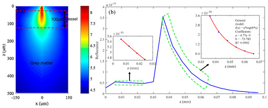
Figure 10.
(a) CW fluence extracted at plane y = 0 μm; (b) the backscattered signal collected by the detector and the fitting results.
Table 6.
Fitting results and calculated C, Y, and S in near-infrared waveband.
In the simulations of this paper, we did not simulate the OCT signals of all wavelengths within the spectral bandwidth of the light source but thought that the extinction coefficient is homogeneous within a certain spectral width, which undoubtedly leads to certain errors. In the visible-light waveband, the maximum wavelength bandwidth set in this work was 15 nm, which has proven to be reasonable [36]. In addition, the impacts of the STFT process on functional sensing were not studied. We will optimize the MMC-OCT program to simulate the complete imaging process of the spectroscopic OCT in future researches.
4. Conclusions
In this study, we analyzed the application of OCT to the fields of brain tissue structural and functional imaging using a model of mesh-based Monte Carlo for OCT (MMC-OCT). We first verified that the MMC-OCT model used in this paper is an effective analytical tool for brain researches through simulations of structural imaging. Then, through theoretical analysis and simulation of functional sensing, we found that the measurement accuracy of hemoglobin concentration C, oxygen saturation Y, and scattering coefficient S can be optimized by reasonable selection of wavelengths. Finally, we proposed the following optimization schemes for imaging vascular structure and cerebral cortex in brain tissue: When imaging small-sized blood vessels, we can reasonably select three wavelengths to resolve C, Y, and S. When imaging the cerebral cortex and the spatial resolution requirement is not high, the method of fitting with multi-wavelength data should be used; when the spatial resolution requirement is high, the measurement accuracy of C, Y, and S can be improved by roughly predicting their ranges in advance to select the appropriate wavelengths for calculation. What is more, these methods are also suitable for other complex 3D bio-tissues. In particular, the method of wavelength selection is also applicable to other optical imaging modalities such as photoacoustic imaging [37], near infrared multispectral imaging [19], etc. In the future, we will provide the whole set of codes and a small guidance for reproducing the results of simulations presented in this manuscript, which provides an analytical method for studying the brain tissue and other complex 3D bio-tissues.
Author Contributions
Conceptualization, L.Y.; formal analysis, L.Y.; methodology, L.Y. and L.S.; software, L.Y., M.Z. and B.H.; supervision, L.S.; validation, L.Y. and L.S.; writing—original draft, L.Y.; writing—review and editing, L.S., M.Z. and B.H.
Funding
This research received no external funding
Acknowledgments
L.Y., M.Z., and B.H. acknowledge the State Key Laboratory of Precision Measurement Technology and Instruments, Department of Precision Instruments, Tsinghua University for support through a PhD studentship.
Conflicts of Interest
The authors declare no conflict of interest.
References
- Xie, Y.; Harsan, L.A.; Bienert, T.; Kirch, R.D.; Von, E.D.; Hofmann, U.G. Qualitative and quantitative evaluation of in vivo SD-OCT measurement of rat brain. Biomed. Opt. Express 2017, 8, 593–607. [Google Scholar] [PubMed]
- Choi, W.J.; Wang, R.K. Optical coherence tomography imaging of cranial meninges post brain injury in vivo. Chin. Opt. Lett. 2017, 15, 16–19. [Google Scholar]
- Tearney, G.J.; Fukumura, D.; Jain, R.K.; Vakoc, B.J.; Lanning, R.M.; Tyrrell, J.A.; Padera, T.P.; Bartlett, L.A.; Stylianopoulos, T.; Munn, L.L. Three-dimensional microscopy of the tumor microenvironment in vivo using optical frequency domain imaging. Nat. Med. 2009, 15, 1219. [Google Scholar]
- Hillman, C.E.M. Optical brain imaging in vivo: Techniques and applications from animal to man. J. Biomed. Opt. 2007, 12, 051402. [Google Scholar] [CrossRef] [PubMed]
- Villringer, A.; Chance, B. Non-invasive optical spectroscopy and imaging of human brain function. Trends Neurosci. 1997, 20, 435–442. [Google Scholar] [PubMed]
- Chong, S.P.; Merkle, C.W.; Leahy, C.; Radhakrishnan, H.; Srinivasan, V.J. Quantitative microvascular hemoglobin mapping using visible light spectroscopic Optical Coherence Tomography. Biomed. Opt. Express 2015, 6, 1429–1450. [Google Scholar] [PubMed]
- Ji, Y.; Vadim, B. Imaging a full set of optical scattering properties of biological tissue by inverse spectroscopic optical coherence tomography. Opt. Lett. 2012, 37, 4443–4445. [Google Scholar]
- Ahn, Y.C.; Jung, W.; Chen, Z. Quantification of a three-dimensional velocity vector using spectral-domain Doppler optical coherence tomography. Opt. Lett. 2007, 32, 1587–1589. [Google Scholar]
- Zhu, C.; Liu, Q. Review of Monte Carlo modeling of light transport in tissues. J. Biomed. Opt. 2013, 18, 50902. [Google Scholar]
- Wang, L.; Jacques, S.L.; Zheng, L. MCML--Monte Carlo modeling of light transport in multi-layered tissues. Comput. Methods Programs Biomed. 1995, 47, 131–146. [Google Scholar]
- Yao, G.; Wang, L.V. Monte Carlo simulation of an optical coherence tomography signal in homogeneous turbid media. Phys. Med. Biol. 1999, 44, 2307–2320. [Google Scholar] [PubMed]
- Shi, B.; Zhuo, M.; Wang, L.; Liu, T. Monte Carlo modeling of human tooth optical coherence tomography imaging. J. Opt. 2013, 15, 075304. [Google Scholar]
- Periyasamy, V.; Pramanik, M. Importance sampling-based Monte Carlo simulation of time-domain optical coherence tomography with embedded objects. Appl. Opt. 2016, 55, 2921–2929. [Google Scholar] [PubMed]
- Hartinger, A.E.; Nam, A.S.; Isabel, C.C.; Vakoc, B.J. Monte Carlo modeling of angiographic optical coherence tomography. Biomed. Opt. Express 2014, 5, 4338–4349. [Google Scholar] [CrossRef] [PubMed]
- Igor, M.; Mikhail, K.; Vladimir, K.; Risto, M. Simulation of polarization-sensitive optical coherence tomography images by a Monte Carlo method. Opt. Lett. 2008, 33, 1581–1583. [Google Scholar]
- Fang, Q. Mesh-based Monte Carlo method using fast ray-tracing in Plücker coordinates. Biomed. Opt. Express 2010, 1, 165–175. [Google Scholar] [PubMed]
- Yao, R.; Intes, X.; Fang, Q. Generalized mesh-based Monte Carlo for wide-field illumination and detection via mesh retessellation. Biomed. Opt. Express 2015, 7, 171–184. [Google Scholar]
- Yi, J.; Chen, S.; Backman, V.; Zhang, H.F. In vivo functional microangiography by visible-light optical coherence tomography. Biomed. Opt. Express 2014, 5, 3603–3612. [Google Scholar] [PubMed]
- Uludag, K.; Kohl, M.; Steinbrink, J.; Obrig, H.; Villringer, A. Cross talk in the Lambert-Beer calculation for near-infrared wavelengths estimated by Monte Carlo simulations. J. Biomed. Opt. 2002, 7, 51–59. [Google Scholar] [PubMed]
- George, M. Optical constants of water in the 200-nm to 200-μm wavelength region. Appl. Opt. 1973, 12, 555–563. [Google Scholar]
- Leitgeb, R.; Wojtkowski, M.; Kowalczyk, A.; Hitzenberger, C.K.; Sticker, M.; Fercher, A.F. Spectral measurement of absorption by spectroscopic frequency-domain optical coherence tomography. Opt. Lett. 2000, 25, 820–822. [Google Scholar] [CrossRef] [PubMed]
- Bosschaart, N.; Edelman, G.J.; Aalders, M.C.G.; Leeuwen, T.G.V.; Faber, D.J. A literature review and novel theoretical approach on the optical properties of whole blood. Laser Med. Sci. 2013, 29, 453–479. [Google Scholar] [CrossRef]
- Smith, M.H.; Denninghoff, K.R.; Hillman, L.W.; Chipman, R.A. Oxygen Saturation Measurements of Blood in Retinal Vessels during Blood Loss. J. Biomed. Opt. 1998, 3, 296–303. [Google Scholar] [PubMed]
- Delori, F.C. Noninvasive technique for oximetry of blood in retinal vessels. Appl. Opt. 1988, 27, 1113–1125. [Google Scholar] [PubMed]
- Hermann, B.; Bizheva, K.; Unterhuber, A.; Povazay, B.; Sattmann, H.; Schmetterer, L.; Fercher, A.; Drexler, W. Precision of extracting absorption profiles from weakly scattering media with spectroscopic time-domain optical coherence tomography. Opt. Express 2004, 12, 1677–1688. [Google Scholar]
- Faber, D.J.; Aalders, M.C.G.; Mik, E.G.; Hooper, B.A.; van Gemert, M.J.C.; van Leeuwen, T.G. Oxygen saturation-dependent absorption and scattering of blood. Phys. Rev. Lett. 2004, 93, 028102. [Google Scholar] [CrossRef] [PubMed]
- Wang, L.V.; Wu, H.I.; Masters, B.R. Biomedical Optics, Principles and Imaging. J. Biomed. Opt. 2008, 13, 049902. [Google Scholar]
- Matcher, S.J.; Cope, M.; Delpy, D.T. In vivo measurements of the wavelength dependence of tissue-scattering coefficients between 760 and 900 nm measured with time-resolved spectroscopy. Appl. Opt. 1997, 36, 386–396. [Google Scholar]
- Hong, G.; Diao, S.; Chang, J.; Antaris, A.L.; Chen, C.; Zhang, B.; Zhao, S.; Atochin, D.N.; Huang, P.L.; Andreasson, K.I. Through-skull fluorescence imaging of the brain in a new near-infrared window. Nat. Photonics 2014, 8, 723–730. [Google Scholar]
- The Program was Downloaded from Open Source Website and Modified. Available online: http://mcx.space/mmc (accessed on 2 November 2018).
- Siavash, M.; Lima, I.T.; Sherif, S.S. Monte Carlo simulation of optical coherence tomography for turbid media with arbitrary spatial distributions. J.Biomed. Opt. 2014, 19, 046001. [Google Scholar]
- Collins, D.L.; Zijdenbos, A.P.; Kollokian, V.; Sled, J.G.; Kabani, N.J.; Holmes, C.J.; Evans, A.C. Design and construction of a realistic digital brain phantom. IEEE Trans. Med. Imaging 1998, 17, 463–468. [Google Scholar] [PubMed]
- Umeyama, S.; Yamada, T. Monte Carlo study of global interference cancellation by multidistance measurement of near-infrared spectroscopy. J.Biomed. Opt. 2009, 14, 064025. [Google Scholar] [PubMed]
- Kholodnykh, A.I.; Petrova, I.Y.; Larin, K.V.; Massoud, M.; Esenaliev, R.O. Precision of measurement of tissue optical properties with optical coherence tomography. Appl. Opt. 2003, 42, 3027–3037. [Google Scholar] [PubMed]
- Yaroslavsky, A.N.; Schulze, P.C.; Yaroslavsky, I.V.; Schober, R.; Ulrich, F.; Schwarzmaier, H.J. Optical properties of selected native and coagulated human brain tissues in vitro in the visible and near infrared spectral range. Phys. Med. Biol. 2002, 47, 2059–2073. [Google Scholar] [CrossRef] [PubMed]
- Ji, Y.; Qing, W.; Liu, W.; Backman, V.; Zhang, H.F. Visible-light optical coherence tomography for retinal oximetry. Opt. Lett. 2013, 38, 1796–1798. [Google Scholar]
- Yin, G.; Yi, Y. Imaging of hemoglobin oxygen saturation using confocal photoacoustic system with three optical wavelengths. In Proceedings of the Seventh International Conference on Photonics and Imaging in Biology and Medicine, Wuhan, China, 24–27 November 2008; Volume 7280. [Google Scholar]


© 2019 by the authors. Licensee MDPI, Basel, Switzerland. This article is an open access article distributed under the terms and conditions of the Creative Commons Attribution (CC BY) license (http://creativecommons.org/licenses/by/4.0/).