Abstract
This paper proposes a single image haze removal algorithm that shows a marked improvement on the color attenuation prior-based method. Through a vast number of experiments on a wide variety of images, it is discovered that there are problems in the color attenuation prior, such as color distortion and background noise, which arise due to the fact that the priors do not hold true in all circumstances. Successful resolution of these problems using the proposed algorithm shows its superior performance to other state-of-the-art methods in terms of both subjective visual quality and quantitative metrics, on both synthetic and natural hazy image datasets. The proposed algorithm also is computationally friendly, due to the use of an efficient quad-decomposition algorithm for atmospheric light estimation and a simple modified hybrid median filter for depth map refinement.
1. Introduction
The prevalence of consumer cameras and the urgent need for groundbreaking work in surveillance or autonomous driving systems have demanded the rapid development of image/video processing algorithms. Among them, the task of eliminating unwanted-but-inevitable weather phenomena from an image has drawn increasing attention in recent years. Generally, this image processing problem is known as visibility restoration. A myriad of algorithms have been proposed to recover the visual quality of weather-degraded images to be as similar as possible to the original ones taken under clear weather conditions. Low-light image enhancement [1,2,3,4], rain removal [5,6,7,8], and image dehazing [9,10,11,12,13,14,15,16,17,18,19,20,21,22,23,24,25,26,27] are cases in point. Haze removal ones, of all the algorithms developed for visibility restoration, have positive impacts on both photography and computer vision applications. Not only does haze removal function properly in hazy, foggy, or misty weather, but it also is appropriate for removing the effect of yellow dust or dust storm on the captured image. Owing to rapid industrialization and urbanization yellow dust is a topical issue in Eastern Asian countries [28] and there is growing demand for a highly sophisticated visibility restoration algorithm.
Generally, haze removal algorithms are categorized according to the number of input images they need. Due to sufficient input information, multi-image approaches [9,10,11,12] are superior to single-image ones [13,14,15,16,17,18,19,20,21,22,23,24,25,26,27] in terms of performance. Given the difficulty of collecting the external information, however, there is little interest from researchers. Accordingly, recent efforts largely have led to single-image dehazing using two-dimensional images without any external knowledge. Such an algorithm, nonetheless, needs to impose priors on the recovered image, for example, enhanced contrast or less attenuated color [23]. The most popular prior is the Dark Channel Prior (DCP), proposed by He et al. [13], which assumes that there exists a dark pixel in every color channel of the local patch around all pixels. Shortly thereafter, the DCP has been improved in many directions [14,15]. Other alternative priors to DCP are the Color Attenuation Prior (CAP) [20], and a distribution of color pixels in the RGB space [18,21]. Li et al. provided a comprehensive review of these methods [22]. A second approach to dehazing problems is to use machine learning techniques [20,25,27]. The mapping between a hazy image and its depth-correlated haze distribution is learned from data in this context. Nevertheless, the lack of real datasets of hazy images and their corresponding ground truth references imposes a limit on the performance of these methods. Yet a third way of approaching image dehazing problems is to consider dehazing as a traditional image enhancement task [23]. The goal is to produce a good quality dehazed image in lieu of estimating the haze distribution in this case. The means to accomplish this consist of contrast enhancement, Retinex-based and fusion-based techniques.
The haze removal method presented in this paper is an improvement upon CAP in terms of both computational efficiency and the dehazed image’s quality. This is achieved by examining the existing drawbacks of CAP, and then proposing effective solutions for individual ones. The first shortcoming of CAP lies in its data preparation stage when training the depth estimator. The synthetic ground truth depth maps are assumed to be uniformly distributed. Since existing pseudo random number generators cannot guarantee the uniform distribution, however, we propose the enhanced equidistribution that has been validated in our previous work [29,30]. We also propose using a simple low-pass filter to remove the background noise and using a simple linear weight to get rid of the color distortion. Furthermore, the commonly observed dynamic range reduction of the dehazed image is resolved by employing the adaptive tone remapping post-processing [31]. Finally, to lighten the CAP’s intensive computation, the efficient quad-decomposition algorithm is utilized to estimate the atmospheric light and the simple modified hybrid median filter (mHMF) is used to refine the depth map. The next section provides an overview of state-of-the-art dehazing algorithms that are used as benchmarking methods in the evaluation section. Section 3 details the solutions of the proposed algorithm for the shortcomings of CAP. Section 4 presents quantitative and qualitative assessments, while Section 5 concludes the paper.
2. Related Works
To restore the visibility of hazy images, most existing algorithms solve the atmospheric scattering model, proposed by McCartney [32]:
where denotes the spatial coordinates of pixels in the hazy image , the haze-free image as well as the transmission map , and is a constant known as atmospheric light. The first term describes the decay of the scene radiance in the transmission medium and is called direct attenuation. The second term is called airlight and represents the additive distortion of the scene radiance due to the scattered light. Given a hazy image , the most popular method is to impose a specific prior information to infer and . Hence, the atmospheric scattering model can be inverted to find the solution :
2.1. Dark Channel Prior
Through extensive observations of outdoor clear images, He et al. [13] found that at least one of three-color channels had extremely low intensity pixels in most image patches, excluding the sky region. Conversely, the minimum intensity of such pixels is almost equal to zero. Based on this observation, the dark channel of the haze-free image is given by:
where the superscript is a color channel of , is a local patch centered at pixel , and denotes the coordinates of pixels within . Using this equation, we first perform a channel-wise minimum operation to find the pixel minimum channel and then apply a minimum filter to get the dark channel. Assuming that is always positive, we can divide both sides of Equation (1) by :
To estimate the transmission map , is assumed to be constant in local patches [13]: . By applying these two minimum operators to Equation (4), the estimated transmission map is obtained as follows:
since the assumption about the dark channel prior () leads to . The application-based positive constant is added to Equation (6) to optionally keep a small amount of haze for human depth perception [13]. Transmission map estimation requires that is known in advance. The authors first select the top 0.1 percent brightest pixels in the dark channel to estimate . Amongst these pixels, the one with highest intensity in the input image is chosen as the atmospheric light .
Since the authors assumed that is constant in local patches, however, artifact blocks arise in the estimated transmission map. Resolving this problem by using the computationally intensive soft matting [33] resulted in a very slow processing speed. Furthermore, the fact that the DCP may be found when observing a non-sky region can cause color distortion in the sky region of the dehazed image. DCP’s drawbacks brought about a large room for improvement, and there have been several studies to extend the DCP in various directions [14,15].
2.2. Fast Haze Removal with Median Filters
Tarel et al. [16] proposed a fast filtering-based algorithm for visibility restoration whose complexity is a linear function of input image pixels. Using this method, the airlight marked is estimated in lieu of the transmission map. The authors proposed the inference that the airlight can be approximated by a percentage of the difference between the local average and the local standard deviation of the input pixel minimum channel . Additionally, the constraint that must be positive and less than is applied to estimate the airlight [16]:
where and denote the local average and local standard deviation of respectively, and is a constant to control the amount of haze to be removed. The nested median filtering operation in Equation (8) is named median of median along lines [16]. Accompanying the estimated airlight, Equation (1) can be re-written to find the haze-free image as follows:
To recover the scene radiance of , the atmospheric light must be given. The authors stated that the atmospheric light is pure white and can be set to (1, 1, 1) if the white balance in the input image is performed correctly. Accordingly, is computed as:
This method suffers from halo artifacts using a large median filter, however. The median filter tends to blur the image edges with depth discontinuities. To solve this problem, Kim et al. [24] proposed using a modified hybrid median filter in place of the standard median filter to provide better performance at image edges when estimating the airlight. This method will be discussed in Section 2.4.
2.3. Color Attenuation Prior
The transmission map in the atmospheric scattering model is exponentially proportional to the scene depth, and this relationship can be expressed as:
where is the scattering coefficient of the atmosphere, and is the scene depth. The large results in a small in the distant regions. Accordingly, a decrease in the image’s saturation caused by the multiplicative direct attenuation term and an increase in the image’s brightness caused by the additive airlight term lead to a big difference between the image’s saturation and brightness. To contrast, the small in the close regions results in a large , therein lies the cause for the small difference between the image’s saturation and brightness. Hence, Zhu et al. [20] proposed a linear model describing the correlation between the scene depth and the difference between the image’s saturation and brightness:
where and are the image’s brightness value and saturation, respectively; , , are the model’s constant parameters; and is a random variable that denotes the model’s error. The authors employed a simple and efficient supervised learning method for the synthetic training data to learn the coefficients , , and .
The method for estimating the atmospheric light is similar to that of DCP. The depth calculated using Equation (14) is filtered by a minimum filter to reduce the influence of white objects on the accuracy of the estimation process. Then, the top 0.1 percent brightest pixels in the depth map are chosen. Among these pixels, the one with the largest L-2 norm in the input image is selected as the atmospheric light. Since the scene depth is blurred as the result of passing through the minimum filter, it is refined by the guided image filter [34] before substituting into Equation (2) to get the haze-free image . The use of a minimum filter is beneficial to the estimation of atmospheric light, but it creates the unfortunate byproduct of blurring the depth map; therefore, a very large guided image filter must be used, and therein causes CAP’s high computational cost. The block diagram of CAP is depicted in Figure 1, in which the red circle shows the minimum filter effectively reduces the influence of white objects (e.g., a train’s headlight), whilst the pale orange circle indicates that it also blurs the depth map, leading to the use of a very large guided image filter.
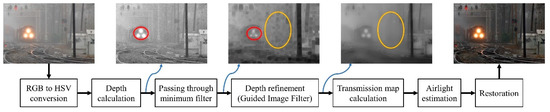
Figure 1.
Block diagram of the haze removal algorithm based on Color Attenuation Prior (CAP).
According to our experiments, CAP works well in most cases but it still suffers some drawbacks, such as background noise, color distortion, and intensive computation. We will delve deeply into these drawbacks and then propose solutions for them in Section 3.
2.4. Hazy Particle Map
Using median filters in Tarel et al.’s dehazing algorithm [16] causes halo artifacts because the standard median filtering is not appropriate for image regions containing edges. This problem can be resolved efficiently using mHMF rather than the standard median filter (SMF), as proposed by Kim et al. [24]. mHMF first computes the medians of three windows: cross, diagonal, and square. Then, the median of these three is selected as the final output. Thus, in flat image regions, mHMF functions in a similar way to SMF and smoothly estimates the hazy particle map (HPM) corresponding to the airlight. The information from the cross and diagonal windows helps mHMF to better preserve the image edges, however, in the abrupt regions with depth discontinuities, resulting in reduced halo artifacts.
Additionally, a sophisticated adaptive tone remapping algorithm [31] also is used, as opposed to the simple tone remapping method used by Tarel et al. [16]. As a result, this algorithm is a significant improvement upon the fast haze removal using median filters, and its hardware design presented by Ngo et al. [35] provides an efficient means of handling large images in real time. An issue arising from the assumption that the atmospheric light is pure white () after local white balance is that noticeable background noise may occur in the dehazed image.
3. Proposed Algorithm
Figure 2 shows the block diagram of the proposed Improved Color Attenuation Prior (ICAP). The abbreviations used in this figure include those for Local White Balance (LWB), Low-Pass Filter (LPF), modified Hybrid Median Filter (mHMF), Minimum Filter (MF), Quad-Decomposition (QD), and Atmospheric Light Estimation (ALE). The five red dotted rectangles represent the functional blocks that distinguish the proposed algorithm from the original CAP. LPF is applied to the image’s saturation channel to remove the background noise. Atmospheric light estimation based upon a quad-decomposition algorithm is effective in lowering the computational complexity and, also, leads to the use of a simple mHMF in place of a very large guided image filter to refine the depth map. An Adaptive Constraints Calculation block strictly constrains the transmission map, preventing the situation where image pixels become negative after dehazing and turn into black pixels. Post-processing blocks include Adaptive Tone Remapping and color converters. They are used to expand the dynamic range of the image after removing haze. We will delve deeply into these differences in following sub-sections.
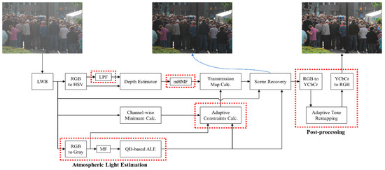
Figure 2.
Block diagram of the proposed Improved Color Attenuation Prior (ICAP).
3.1. New Data Preparation Method for Training Depth Estimator
The training data consisting of hazy images and their corresponding ground truth depth maps are required to correctly learn the coefficients , , and in Equation (14). Unfortunately, the acquisition of an accurate depth map is extremely difficult since there is no reliable means to obtain the scene depth. Therefore, Zhu et al. [20] used a synthetic database to train their proposed linear model. The training data preparation phase can be described in four steps: (i) collecting the haze-free images from image-sharing services like Google Images or Flickr; (ii) generating random depth maps with the standard uniform distribution on the open interval (0, 1); (iii) generating a random global atmospheric light with its value between 0.85 and 1.0; (iv) substituting these variables into the atmospheric scattering model to calculate the synthetic hazy images. Then, the saturation and value channels of these hazy images are used as input data, while the random depth maps are employed as known responses in the supervised learning strategy. Three coefficients in Equation (14) were learned by maximizing the natural logarithm of the likelihood using the stochastic gradient ascent algorithm. Zhu et al. [20] also provided a detailed flowchart showing mathematical expressions for both calculating the partial gradients and updating the coefficients. Figure 3 depicts this data preparation procedure.
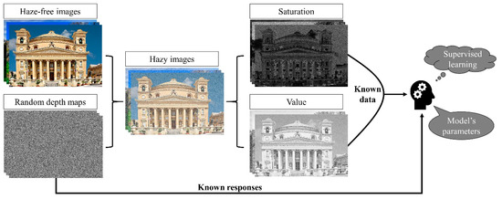
Figure 3.
Data preparation procedure employed in CAP.
Our training data is constructed according to the procedure illustrated in Figure 3 on 500 haze-free images of 500 × 400 uniform size, in which a noticeable improvement in generating random depth maps has been made. To solve the problem that existing pseudo random number generators cannot guarantee a uniform distribution, we adopted the enhanced equidistribution [29,30]. Figure 4a shows the histogram of 200,000 random numbers, corresponding to a 500 × 400 depth map, drawn from the standard uniform distribution on the open interval (0, 1). The numbers are distributed almost uniformly in view, but the standard deviation of the numbers is still greater than zero. Figure 4b is the histogram of the numbers after being modified by the enhanced equidistribution. The current distribution is mostly uniform and is, theoretically, close to the uniform distribution. Preparing training data for CAP’s linear model using the depth maps drawn from the enhanced equidistribution further improves the CAP performance, proven in our previous work [29,30]. Regarding the learning strategy, since the stochastic gradient ascent algorithm is considerably slow, we utilize the mini-batch gradient ascent algorithm with the following hyper-parameters: the global learning rate of 1e-5; the batch size of 3 images; and the epoch number of 1000. The best result we obtained is that , , and . These parameters will be used for the evaluation in Section 4.
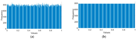
Figure 4.
Histograms of 200,000 random numbers: (a) drawn from the standard uniform distribution and (b) drawn from the enhanced equidistribution.
3.2. Adaptive Constraints for Transmission Map
The transmission map calculated from the estimated depth map using Equation (13) is called the raw transmission map, and it is usually not good enough for haze removal. Zhu et al. [20] implicitly refined the raw transmission map by refining the depth map using a very large guided image filter, and then simply constrained the transmission map between two fixed boundaries: 0.05 and 1. The small-global limit (0.05) indicates that image regions with this lower bound will be heavily dehazed, possibly resulting in background noise or color distortion, which can be seen in Section 4.2 of the qualitative evaluation. The depth map is not utilized in this paper to estimate the atmospheric light, as will be discussed in Section 3.5. Hence, we can get rid of the guided image filter since the depth map is not passed through the minimum filter. Instead, the simple mHMF can be employed to refine the estimated depth map. Additionally, we also develop two adaptive constraints from the atmospheric scattering model to refine the transmission map. To begin with, the transmission map can be derived from Equation (1) as:
When the haze-free image is correctly recovered, its value will lie within the range 0 to 1 (normalized value). Hence, applying the condition to Equation (15) yields:
since the atmospheric light is constant in the image. Equation (17) is the first adaptive constraint for the raw transmission map.
The second adaptive constraint is inspired by the mean and standard deviation definitions in statistics. To simplify, haze removal is the subtraction of haze from a hazy image, where the amount of subtraction is controlled by the values of the transmission map. The smaller these values are, the more haze that is removed, and therein lies the cause of the dehazed image’s usually low intensities. Pixel values within dark images are limited to zero in case they become negative after dehazing. These pixels are called black pixels [36]. To prevent black pixels from occurring in the dehazed image, the second constraint specifies that the image local average should be greater than or equal to the image local standard deviation, as follows:
where is a constant to control the deviation, and the empirical choice of is used for the evaluation in Section 4. When the input image is mostly quite dark, its pixels are highly likely to become black pixels after removing haze. The constant , in such a case, can be set to a value greater than 1.0 (e.g., 2.0, 2.5, or 3.0) to tighten the constraint. The image local average, as well as local standard deviation, can be derived from Equation (2) using its linearity, as follows:
Substituting Equations (19) and (20) into Equation (18) results in the second adaptive constraint, as:
Combining the result with the first constraint yields the complete constraint on the transmission map, as:
which is preferred over the simple constraint used in the original CAP due to the adaptive lower limit derived from the effort to prevent undershoots and reduce the number of black pixels.
3.3. Background Noise Removal
Background noise is a common problem for all the haze removal algorithms mentioned in Section 2. Figure 5 illustrates the input hazy image, which is from the Image and Vision Computing (IVC) image dataset [37], and the output dehazed images from DCP, filtering-based fast dehazing (FFD), CAP, and HPM. The enlarged regions show background noise after removing the haze owing to various reasons. Using DCP, it is found when observing image patches excluding the sky. Using FFD and HPM, the assumption that the atmospheric light can be set to (1, 1, 1) causes the noise. Since the contribution of the atmospheric light in the formation of hazy images is additive according to Equation (1), dehazing means this kind of unwanted contribution must be subtracted. As a result, using the maximum values of atmospheric light indicates that the subtraction is performed excessively and, thus, highly likely gives rise to background noise.
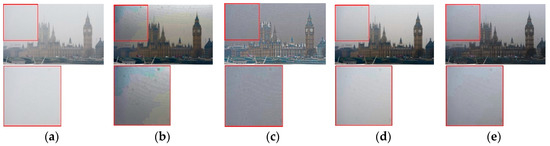
Figure 5.
Results of different methods on a real hazy scene and their corresponding zoomed-up sky region: (a) input hazy image; (b) Dark Channel Prior (DCP); (c) Filtering-based Fast Dehazing (FFD); (d) CAP; (e) Hazy Particle Map (HPM).
Conversely, the cause of CAP background noise is related to the spike-like noise in the saturation channel. To delve deeply into this, a thorough examination is in order. Figure 6 shows another hazy image from the IVC dataset, its corresponding estimated depth map, and the recovered haze-free image. It is evident that the background noise in the marked region is carried over into the dehazed image, owing to the linearity of the atmospheric scattering model. To find the cause of the background noise, we looked at the saturation, brightness, and depth values of line 247, as depicted in Figure 7a. This shows that small or spike-like noise in saturation data creates the corresponding noise in the depth map of the CAP linear model. This noise eventually makes the background noise in the dehazed image and can be removed by using a low-pass filter. Figure 7b shows that the noise in the saturation data has been removed successfully, creating smooth depth data. Figure 8 shows the estimated depth maps before and after applying the low-pass filter. It is evident that the background noise marked by the red rectangle is filtered out efficiently. This feature clearly distinguishes the proposed ICAP from the original CAP. The coefficients and one-dimensional frequency response of the low-pass filter are illustrated in Figure 9.
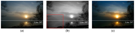
Figure 6.
An example where background noise occurred after dehazing: (a) hazy image; (b) estimated depth map; (c) dehazed image.
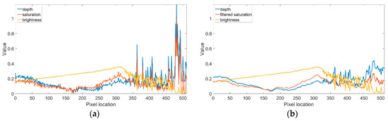
Figure 7.
Plot of image line 247 data across the noisy region: (a) before applying the low-pass filter and (b) after applying the low-pass filter.
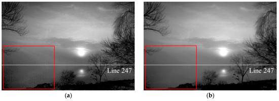
Figure 8.
Estimated depth maps: (a) before applying the low-pass filter and (b) after applying the low-pass filter.
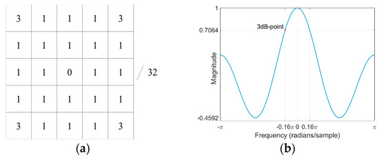
Figure 9.
Background noise removal low-pass filter’s coefficients and one-dimensional frequency response: (a) coefficients and (b) one-dimensional frequency response.
3.4. Color Distortion
Another drawback of CAP is that it does not work well in the dark image region, where both the saturation and brightness are low. Thus, CAP misinterprets this region as the close region, resulting in a small estimated depth value (close to zero), subsequently leading to a large transmission map value (close to one) according to Equation (13). Figure 10 shows this.
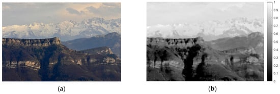
Figure 10.
CAP misinterprets the dark region as the close region: (a) hazy image and (b) estimated depth map.
To determine the cause of color distortion, five pixels in the dark region of the input hazy and dehazed images have been taken into consideration, as illustrated in Figure 11. When the scene radiance of the haze-free image is recovered using Equation (2), the pixel values within the dark image region marked A, B, C, D, and E will be decreased slightly or sometimes unchanged. Table 1 shows the blue channel has larger values, in comparison to the red and green channels. Following dehazing, the small decrease has a negligible impact on the large blue channel, but significant impact on the small red and green channels. Therefore, the dark regions in the dehazed image look blue, as shown in Figure 11b.
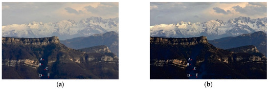
Figure 11.
Pixels in dark region marked A, B, C, D, and E of: (a) hazy image and (b) dehazed image.

Table 1.
Red-Green-Blue (RGB) values of dark pixels in Figure 11.
Regarding this kind of color distortion, one solution is to add a weight factor to make the color in the dark image region consistent, that is, going darker after removing haze. Adding to that, the weight factor is set in linear form to lighten the computational complexity of the proposed algorithm. Hence, we propose an adaptive weight factor depicted in Figure 12, where denotes the starting value of , and represents the depth value that specifies the close region. We have found empirically that the values of and are effective in providing visually-pleasing results for almost all images tested for the proposed algorithm. The formula of and the revised formula for recovering scene radiance are as follows:
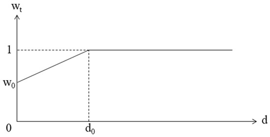
Figure 12.
Adaptive weight factor for resolving color distortion.
Figure 13 shows dehazed images before and after applying the proposed weight factor . The difference is noticeable, since adding forces the color of the dark region to go darker, which is the desired effect according to the atmospheric scattering model. This is another obvious distinction between the proposed ICAP and the original CAP.
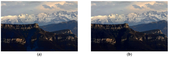
Figure 13.
Dehazed images: (a) before applying and (b) after applying .
3.5. Atmospheric Light Estimation
Methods for estimating the atmospheric light in recent haze removal algorithms usually suffer from one of two major issues: high cost in terms of computational complexity, and incorrectly taking pixels belonging to white objects into consideration. DCP’s or CAP’s atmospheric light estimation suffers from the former, and even the latter in specific cases, for example. This is because finding the pixel in the hazy image that corresponds to the brightest pixel amongst a percentage of pixels within a transmission map or depth map requires sorting all pixels and then searching over the selected ones. Additionally, if the percentage is not chosen carefully, image pixels within white objects may be included mistakenly in the estimation process. Using FFD’s atmospheric light estimation approach, setting . to (1, 1, 1) after white balance absolutely does not work for images containing white objects therein. Thus, we have decided to use the quad-decomposition algorithm [19], which has been proven to be an efficient and fast estimation method.
This algorithm operates on the image’s luminance channel which, to prevent the unwanted influence of white objects, must be processed by a minimum filter in advance. Then, it iteratively divides the image’s luminance into quarters and selects a quarter with the largest average luminance, until the quarter’s size is less than a predetermined value. Using the finally selected quarter, a pixel with minimum Euclidean distance to (1, 1, 1) coordinate in the RGB space is chosen as the atmospheric light. Figure 14a shows an image in the IVC dataset where CAP fails to estimate the atmospheric light correctly. The red pixels are those corresponding to 0.1 % of the farthest pixels in the depth map, and the chosen one is the pixel in the train’s front light. Furthermore, CAP needs to search through the entire spatial area of an image to find these pixels. To contrast, since the train’s front light cannot dominate the average brightness in the image quarters, quad-decomposition does not take it into consideration. Simultaneously, the search area also is reduced iteratively by a factor of four for accurate estimation. The red dot in Figure 14b refers to a pixel being chosen as the atmospheric light, but it is enlarged for visual convenience.
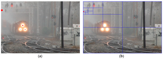
Figure 14.
Atmospheric light estimation: (a) CAP and (b) the proposed algorithm.
3.6. Adaptive Tone Remapping
The dehazing algorithm often results in a low-dynamic range image, owing to the fact that computations can produce results out of the normalized range from 0 to 1. Tarel et al. [16] employed a simple tone mapping that solely operates on the luminance channel to resolve this problem. We make use of an efficient adaptive tone remapping method, proposed by Cho et al. [31], in this work. Not only is the luminance enhanced, the color also is emphasized, according to the ratio of the enhanced luminance to the original luminance.
where denotes the enhanced luminance, the input luminance, the luminance gain, the adaptive luminance weight, the emphasized color, the input color, the color gain, and the adaptive color weight. Cho et al., [31] adopted an adaptive limit point, which is calculated according to the cumulative distribution function of the input luminance, to formulate the luminance gain as a nonlinear power function. The adaptive luminance weight is a simple linear function where the input luminance is the independent variable and itself is the dependent variable. The color gain is defined as the multiplication of the input color and the ratio between the enhanced luminance and the input luminance. The adaptive color weight is the piecewise linear function consisting of three line segments, in which the first and the third lines are two thresholds. Readers can refer to Choe et al., [31] for a more detailed description and computational formulae.
4. Evaluations
This section provides the comparative evaluation of the proposed ICAP and several state-of-the-art haze removal algorithms, including DCP, CAP, FFD, and HPM, both in terms of quantitative and qualitative assessments.
4.1. Quantitative Evaluation
4.1.1. Metrics
The selection of evaluation metrics depends upon the collection of test images. To carry out an extensive evaluation, we employ both synthetic [36,38] and real hazy images [37,39,40]. The following sub-sections present details about the evaluation of these sets of images.
4.1.2. Synthetic Datasets
Foggy Road Image DAtabase 2 (FRIDA2) [36] and D-HAZY [38] are two synthetic datasets that contain pairs of ground truth reference images and hazy images of the same scene. There are 264 synthetic hazy images of 66 road scenes in the FRIDA2 dataset and they are generated completely by computer graphics. Each road scene comprises a ground truth reference and four associated hazy images corresponding to four different kinds of haze: homogeneous, heterogeneous, cloudy homogeneous, and cloudy heterogeneous. This dataset is designed for Advanced Driver Assistance Systems (ADAS) [38]. Since FRIDA2 solely contains computer graphic generated scenes, it may not be valid for real scenarios. Accordingly, an additional D-HAZY dataset consisting of real ground truth reference images and synthesized hazy ones has come into use. It contains over 1400 images of real scenes and their corresponding depth maps captured by a Microsoft Kinect camera. Then, the atmospheric scattering model is used with the assumptions that the atmospheric light and haze density are both uniform to synthesize hazy images.
As these datasets have ground truth reference images, Structural SIMilarity (SSIM) [41], Tone-Mapped image Quality Index (TMQI) [42], and Feature SIMilarity extended to color image (FSIMc) [43] are employed in an evaluation. Additionally, Fog Aware Density Evaluator (FADE) [44], a learned metric predicting the haze density in a scene, also is used to assess the visibility of the scene after removing haze. The smaller FADE is, in this context, the larger the amount of haze that has been removed.
It is supposed that and are two nonnegative image luminance signals. The SSIM measure of two images is calculated as follows:
where (, ) and (, ) are the local average and standard deviation of , , respectively; and are constants for avoiding the instability when () and () are very close to zero; and is the correlation coefficient between () and (). The value of SSIM ranges from 0 to 1, in which higher SSIM means two images are more structurally similar.
Moreover, Equation (28) gives the formula of TMQI, where and now denote two color images. is the statistical naturalness measure, is the overall structural fidelity score, is used to adjust the relative importance of these two components, and and determine their sensitivities. Even though and are two color images, TMQI only evaluates their grayscale channel to assess the structural information preserving characteristics. TMQI takes on values within the range [0, 1], in which the higher, the better:
FSIMc is developed based on the observation that a human visual system perceives an image mainly according to its low-level features, such as the phase congruency, the image gradient magnitude, and the chrominance similarity. FSIMc is calculated by:
where denotes the combined similarity measure of the phase congruency and the gradient magnitude similarities between two images, the chrominance similarity measure, the coefficient weighting the importance of in the overall similarity between and , and is a positive constant for adjusting the importance of the chrominance component. Looking at Equation (29), means the whole image domain. Since both SSIM and TMQI are designed to evaluate grayscale images only, an additional FSIMc is used to conduct a thorough assessment. Similarly, FSIMc lies between 0 and 1, where the higher FSIMc means that the compared image resembles the reference image to a greater degree.
FADE is a referenceless evaluation metric based on natural scene statistics (NSS), fog aware statistical features (FASFs), and Mahalanobis distance. The feature domain is defined based on a total of twelve features, including NSS and FASFs [44]. Choi et al. [44] first collected 500 hazy images and another 500 haze-free images. The features extracted from these two image groups were then individually fitted to the multivariate Gaussian (MVG) model to calculate their corresponding mean vector (, ) and covariance matrix (, ), respectively. To access the perceptual haze density of a particular input image, its extracted features also are fit to MVG model. The mean vector () and covariance matrix () are then employed to calculate the Mahalanobis distances from input image to hazy image group () and haze-free image group (), as shown in Equations (30) and (31). Finally, FADE is calculated as the ratio in Equation (32) and then has positive values, where the smaller is the better.
Table 2 and Table 3 display the average SSIM, TMQI, FSIMc, and FADE results on the FRIDA2 and D-HAZY datasets, respectively. The best result is marked with bold. Since the luminance information contributes toward the calculation of SSIM, TMQI, and FSIMc, the noticeable background noise of HPM and the halo artifacts of FFD increase these quantitative scores to a certain extent. Thus, they exhibit fairly good performance in terms of SSIM, TMQI, and FSIMc, but not FADE. Alternately, CAP possesses the best FADE score and high TMQI and FSIMc. This is because CAP often excessively removes haze from hazy images, bringing about better colorfulness restoration. Removing too much haze also causes loss of image details, however, resulting in CAP’s low SSIM. Regarding DCP, as FRIDA2 dataset contains images of a road scene with sky regions, DCP shows poor performance. The proposed ICAP is the best performing method under the SSIM, TMQI, and FSIMc metrics and the second-best method in terms of FADE. It is attributed to the adaptive constraints on the lower limit of a transmission map, which avoids the excessive haze removal that occurs in CAP. According to Table 3, however, ICAP is only the third best under the SSIM and FSIMc metrics, and the best under the FADE metric. This is because D-HAZY is a kind of biased dataset that solely consists of indoor images, while our proposed ICAP has been tuned to gain best performance in both outdoor and indoor scenes. The fact that DCP performs best on the D-HAZY dataset shows that DCP is a fine prior for indoor dehazing, and our experiment results are consistent with those presented by Ancuti et al. [38].
Table 2.
Average Structural Similarity (SSIM), Tone-Mapped image Quality Index (TMQI), Feature Similarity extended to color image (FSIMc), and Fog Aware Density Evaluator (FADE) results on Foggy Road Image Database 2 (FRIDA2) dataset.
Table 3.
Average SSIM, TMQI, FSIMc, and FADE results on the D-HAZY dataset.
4.1.3. Real Datasets
The IVC [37], O-HAZE [39], and I-HAZE [40] image datasets are used in this section to assess the dehazing performance on hazy images of the real scene. The IVC dataset contains 25 hazy images of people, animals, landscape, indoor, and outdoor real images and does not contain their corresponding ground-truth haze-free images. Conversely, the O-HAZE dataset consists of 45 pairs of hazy and haze-free images of outdoor scenes, and the I-HAZE dataset comprises 30 pairs of hazy and haze-free images of indoor scenes. The haze in the hazy scenes of O-HAZE and I-HAZE datasets is created by the vapor generator.
Due to the lack of reference images in the IVC dataset, the rate of new visible edges (), the quality of the contrast restoration (), proposed by Hautiere et al. [45], and FADE are used to evaluate the performance of dehazing approaches. Since O-HAZE and I-HAZE possess reference images, SSIM, TMQI, FSIMc, and FADE are used as in the preceding section. The values of and are determined by the following equations:
where and denote the numbers of the set of visible edges in the restored image and the original image, respectively. Thus, assesses the ability of an algorithm to restore edges that are visible in the restored image, but are not in the original one [45]. Using Equation (34), denotes the set of visible edges in the restored image, and is the ratio determining the improvement of visibility level. Therefore, higher values of and are desired in an image processing task.
Table 4, Table 5 and Table 6 show the average evaluation metric results on the IVC, O-HAZE, and I-HAZE datasets. Similarly, the best results are shown in bold. The values of and are directly proportional to the number of newly restored edges in the dehazed image. Hautiere et al. [45], however, stated that any set of edges which have a local contrast above 5% are assumed to be the visible edges. Accordingly, in methods susceptible to the background noise, like FFD and HPM, it appears that noises may be misinterpreted and then adversely affect the accuracy of and . Hence, even though ICAP has lower and results than FFD and HPM, it may still be the best performing method when considering the background noise resistant characteristics. This can be observed in the qualitative evaluation in the next section. Using the O-HAZE dataset, our proposed ICAP is the best method in terms of TMQI and FADE, and the second best under SSIM and FSIMc metrics. The dehazing performance is even more impressive on the I-HAZE dataset, where the proposed ICAP exhibits the best dehazing power under SSIM, TMQI, and FSIMc metrics. The clear superiority of ICAP over CAP is attributed to all the improvements presented in Section 3. The adaptive linear weight for handling color distortion makes ICAP outperform CAP in dark areas, resulting in smaller FADE, except for in the I-HAZE dataset, where FADE = 0.8053 may be too low, causing loss of image details. This, coupled with the adaptive constraints on the transmission map and the background noise reduction, leads to the higher TMQI and FSIMc. Adding to that, the adaptive tone remapping post-processing also contributes toward the high scores of TMQI and FSIMc.
Table 4.
Average rate of new visible edges (e), quality of contrast restoration (r), and FADE results on the Image and Vision Computing (IVC) dataset.
Table 5.
Average SSIM, TMQI, FSIMc, and FADE results on the O-HAZE dataset.
Table 6.
Average SSIM, TMQI, FSIMc, and FADE results on the I-HAZE dataset.
4.2. Qualitative Evaluation
Figure 15 presents a hazy scene of landscape, to visually assess the dehazing performance of the proposed ICAP and other benchmarking methods. It is evident that, in this case, the methods with higher haze-removal ability are the DCP and ICAP. Considering the red cropped regions, it is observed that color distortion occurs in FFD, CAP, and HPM, while DCP and ICAP produce results that are consistent with the atmospheric scattering model. The green cropped regions, however, show that only the proposed ICAP has the ability to correctly remove haze in the sky region. DCP, due to its well-known drawback in handling the sky region, introduces an unrealistic color shift, turning the sky to yellow. The same problem also can be seen in FFD, CAP, and HPM, in which HPM also produces additional background noise.
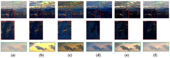
Figure 15.
Qualitative assessment of different algorithms on a real hazy scene of landscape: (a) hazy image, dehazed images and corresponding zoomed-up regions of (b) DCP, (c) FFD, (d) CAP, (e) HPM, and (f), the proposed ICAP.
Figure 16 shows an image of a hazy outdoor scene as a second example. Since this image mainly contains non-sky regions, DCP and ICAP share the top dehazing performance. The zoomed-up color chart regions reveal that CAP and HPM exhibit lower dehazing power than the other three methods, since, not only do they suffer from color distortion, they also lose the details of the grass. Alternately, the FFD method produces a visually acceptable result, but it still has halo artifacts at the small edges of grass and color distortion, which can be seen in the first element of the first and third rows of the color chart. Regarding the green zoomed-up regions, even though FFD exhibits the best performance in restoring details, the unwanted halo artifacts in other regions lower its dehazing power in general. DCP also performs well in this region, but it tends to darken the image by removing too much haze, which may fade the details in dark regions. Thus, the proposed ICAP, which produces visually satisfactory results, can be considered as a high-performance method in haze removal. Figure 17 illustrates other examples of the real hazy scene, to demonstrate the dehazing capability of ICAP and other methods.
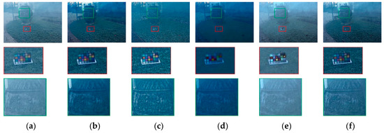
Figure 16.
Qualitative assessment of different algorithms on a real hazy outdoor scene: (a) hazy image, dehazed images and corresponding zoomed-up regions of (b) DCP, (c) FFD, (d) CAP, (e) HPM, and (f), the proposed ICAP.
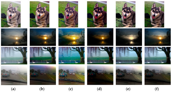
Figure 17.
Qualitative assessment of different algorithms on real-world scenes: (a) hazy images; (b) results of DCP; (c) results of FFD; (d) results of CAP; (e) results of HPM; and (f) results of the proposed ICAP.
4.3. Computational Complexity Comparison
Table 7 summarizes the computational complexity based on the CPU times using the above-mentioned algorithms. The best results are marked bold. They were all programmed via MATLAB R2019a and tested on a Core i7-6700 CPU (3.4 GHz) with 32GB RAM. It is evident that for any image sizes ranging from 320 × 240 to 4096 × 2160, the proposed ICAP always possesses the fastest processing speed. DCP exhibits the poorest performance, due largely to the computationally intensive soft-matting. The processing time of DCP for a 4096 × 2160 image could not be even measured to due insufficient RAM. FFD is better than DCP in terms of processing speed, since filtering techniques are exploited in place of soft-matting. HPM is about twice as fast as FFD. Conversely, CAP is only faster than the slowest DCP in this comparison because it uses a very large guided image filter continuously after a large minimum filter. The proposed ICAP reduces the processing time of CAP by more than six times. The advantage of processing speed is attributed to the clever use of a quad-decomposition algorithm, mHMF, simple low-pass filter, and linear form of adaptive weight.
Table 7.
Processing time in seconds of Dark Channel Prior (DCP), Filtering-based Fast Dehazing (FFD), Color Attenuation Prior (CAP), Hazy Particle Map (HPM), and Improved Color Attenuation Prior (ICAP).
5. Conclusions
An improvement upon the Color Attenuation Prior-based dehazing method, termed ICAP, has been developed. By carefully examining the advantages and disadvantages of CAP, as well as other state-of-the-art haze removal algorithms, ICAP is proposed to overcome some of the existing limitations. First of all, owing to the lack of datasets containing pairs of hazy and haze-free images of real scenes, synthetic datasets were used to train the depth estimator. We, therefore, proposed the enhanced equidistribution, in lieu of the standard uniform distribution, to create the synthetic training dataset. This was validated in our previous work [29,30], revealing that the new synthetic training dataset brings about a significant improvement in dehazing performance. Additionally, to reduce the computational complexity of the proposed algorithm, the fast and efficient quad-decomposition algorithm that operates on the luminance channel was utilized for atmospheric light estimation. As a result, the simple mHMF can be used to refine the depth map, instead of a very large guided image filter. Furthermore, the background noise issue that arose in the CAP was successfully traced to the noise in the saturation channel, which was filtered easily by a low-pass filter. Finally, the well-known color distortion existing in many contemporary haze removal methods also was resolved, by using the adaptive linear weight.
ICAP exhibits good performance in comparison to other benchmarking methods for the task of visibility restoration. This has been verified through extensive experiments on both synthetic and real datasets. The quantitative results show that there is large room for improvement in the haze removal algorithm.
Author Contributions
Conceptualization, G.-D.L. and B.K.; data curation, D.N.; validation, D.N. and B.K.; writing-original draft, D.N. and B.K.; supervision, B.K.
Funding
This research was supported by research funds from Dong-A University, Busan, South Korea.
Conflicts of Interest
The authors declare no conflict of interest.
References
- Arici, T.; Dikbas, S.; Altunbasak, Y. A Histogram Modification Framework and Its Application for Image Contrast Enhancement. IEEE Trans. Image Process. 2009, 18, 1921–1935. [Google Scholar] [CrossRef] [PubMed]
- Huang, S.; Cheng, F.; Chiu, Y. Efficient Contrast Enhancement Using Adaptive Gamma Correction with Weighting Distribution. IEEE Trans. Image Process. 2013, 22, 1032–1041. [Google Scholar] [CrossRef] [PubMed]
- Albu, F.; Vertan, C.; Florea, C.; Drimbarean, A. One Scan Shadow Compensation and Visual Enhancement of Color Images. In Proceedings of the 2009 16th IEEE International Conference on Image Processing (ICIP), Cairo, Egypt, 7–10 November 2009; pp. 3133–3136. [Google Scholar]
- Ngo, D.; Kang, B. Preprocessing for High Quality Real-time Imaging Systems by Low-light Stretch Algorithm. J. Inst. Korean. Electr. Electron. Eng. 2018, 22, 585–589. [Google Scholar]
- Garg, K.; Nayar, S.K. Detection and Removal of Rain from Videos. In Proceedings of the 2004 IEEE Computer Society Conference on Computer Vision and Pattern Recognition(CVPR), Washington, DC, USA, 27 June–2 July 2004; pp. 528–535. [Google Scholar]
- Luo, Y.; Xu, Y.; Ji, H. Removing Rain from a Single Image via Discriminative Sparse Coding. In Proceedings of the 2015 IEEE International Conference on Computer Vision (ICCV), Santiago, Chile, 7–13 December 2015; pp. 3397–3405. [Google Scholar]
- Wang, Y.; Chen, C.; Zhu, S.; Zeng, B. A Framework of Single-Image Deraining Method Based on Analysis of Rain Characteristics. In Proceedings of the 2016 IEEE International Conference on Image Processing (ICIP), Phoenix, AZ, USA, 25–28 September 2016; pp. 4087–4091. [Google Scholar]
- Kim, J.; Lee, C.; Sim, J.; Kim, C. Single-Image Deraining Using an Adaptive Nonlocal Means Filter. In Proceedings of the 2013 IEEE International Conference on Image Processing, Melbourne, Australia, 15–18 September 2013; pp. 914–917. [Google Scholar]
- Shwartz, S.; Namer, E.; Schechner, Y.Y. Blind Haze Separation. In Proceedings of the 2006 IEEE Computer Society Conference on Computer Vision and Pattern Recognition (CVPR’06), New York, NY, USA, 17–22 June 2006; Volume 2, pp. 1984–1991. [Google Scholar]
- Kopf, J.; Neubert, B.; Chen, B.; Cohen, M.; Cohen-Or, D.; Deussen, O.; Uyttendaele, M.; Lischinski, D. Deep Photo: Model-Based Photograph Enhancement and Viewing. ACM Trans. Graph. 2008, 27, 116:1–116:10. [Google Scholar] [CrossRef]
- Xia, P.; Liu, X. Image dehazing technique based on polarimetric spectral analysis. Opt. Int. J. Light Electron Opt. 2016, 127, 7350–7358. [Google Scholar] [CrossRef]
- Zhang, W.; Liang, J.; Ren, L. Haze-removal polarimetric imaging schemes with the consideration of airlight’s circular polarization effect. Optik 2019, 182, 1099–1105. [Google Scholar] [CrossRef]
- He, K.; Sun, J.; Tang, X. Single Image Haze Removal Using Dark Channel Prior. IEEE Trans. Pattern Anal. Mach. Intell. 2011, 33, 2341–2353. [Google Scholar] [PubMed]
- Zhu, Y.; Tang, G.; Zhang, X.; Jiang, J.; Tian, Q. Haze removal method for natural restoration of images with sky. Neurocomputing 2018, 275, 499–510. [Google Scholar] [CrossRef]
- Lee, S.; Yun, S.; Nam, J.-H.; Won, C.S.; Jung, S.-W. A review on dark channel prior based image dehazing algorithms. J. Image Video Proc. 2016, 2016, 4. [Google Scholar] [CrossRef]
- Tarel, J.; Hautière, N. Fast visibility restoration from a single color or gray level image. In Proceedings of the 2009 IEEE 12th International Conference on Computer Vision, Kyoto, Japan, 29 September–2 October 2009; pp. 2201–2208. [Google Scholar]
- Nishino, K.; Kratz, L.; Lombardi, S. Bayesian Defogging. Int. J. Comput. Vis. 2012, 98, 263–278. [Google Scholar] [CrossRef]
- Fattal, R. Dehazing Using Color-Lines. ACM Trans. Graph. 2014, 34, 13:1–13:14. [Google Scholar] [CrossRef]
- Park, D.; Park, H.; Han, D.K.; Ko, H. Single image dehazing with image entropy and information fidelity. In Proceedings of the 2014 IEEE International Conference on Image Processing (ICIP), Paris, France, 27–30 October 2014; pp. 4037–4041. [Google Scholar]
- Q Zhu, Q.; Mai, J.; Shao, L. A Fast Single Image Haze Removal Algorithm Using Color Attenuation Prior. IEEE Trans. Image Process. 2015, 24, 3522–3533. [Google Scholar]
- Berman, D.; Treibitz, T.; Avidan, S. Non-Local Image Dehazing. In Proceedings of the 2016 IEEE Conference on Computer Vision and Pattern Recognition (CVPR), Las Vegas, NV, USA, 27–30 June 2016; pp. 1674–1682. [Google Scholar]
- Li, Y.; You, S.; Brown, M.S.; Tan, R.T. Haze visibility enhancement: A Survey and quantitative benchmarking. Comput. Vis. Image Underst. 2017, 165, 1–16. [Google Scholar] [CrossRef]
- Galdran, A. Image dehazing by artificial multiple-exposure image fusion. Signal Process. 2018, 149, 135–147. [Google Scholar] [CrossRef]
- Kim, G.; Lee, S.; Kang, B. Single Image Haze Removal using Hazy Particle Maps. IEICE Trans. Fundam. Electron. Commun. Comput. Sci. 2018, 101, 1999–2002. [Google Scholar] [CrossRef]
- Tang, K.; Yang, J.; Wang, J. Investigating Haze-Relevant Features in a Learning Framework for Image Dehazing. In Proceedings of the 2014 IEEE Conference on Computer Vision and Pattern Recognition, Columbus, OH, USA, 23–28 June 2014; pp. 2995–3002. [Google Scholar]
- Cai, B.; Xu, X.; Jia, K.; Qing, C.; Tao, D. DehazeNet: An End-to-End System for Single Image Haze Removal. IEEE Trans. Image Process. 2016, 25, 5187–5198. [Google Scholar] [CrossRef] [PubMed]
- Ren, W.; Liu, S.; Zhang, H.; Pan, J.; Cao, X.; Yang, M.-H. Single Image Dehazing via Multi-scale Convolutional Neural Networks. In Proceedings of the Computer Vision—ECCV 2016; Leibe, B., Matas, J., Sebe, N., Welling, M., Eds.; Springer International Publishing: Cham, Switzerland, 2016; pp. 154–169. [Google Scholar]
- Zhao, M.; Xiu, G.; Qiao, T.; Li, Y.; Yu, J. Characteristics of Haze Pollution Episodes and Analysis of a Typical Winter Haze Process in Shanghai. Aerosol Air Qual. Res. 2016, 16, 1625–1637. [Google Scholar] [CrossRef]
- Ngo, D.; Kang, B. Improving Performance of Machine Learning-based Haze Removal Algorithms with Enhanced Training Database. J. Ins. Korean. Electr. Electron. Eng. 2018, 22, 948–952. [Google Scholar]
- Ngo, D.; Kang, B. A New Data Preparation Methodology in Machine Learning-Based Haze Removal Algorithms. In Proceedings of the 2019 International Conference on Electronics, Information, and Communication (ICEIC), Auckland, New Zealand, 22 January 2019; pp. 1–4. [Google Scholar]
- Cho, H.; Kim, G.-J.; Jang, K.; Lee, S.; Kang, B. Color Image Enhancement Based on Adaptive Nonlinear Curves of Luminance Features. JSTS J. Semicond. Technol. Sci. 2015, 15, 60–67. [Google Scholar] [CrossRef]
- McCartney, E.J. Optics of the Atmosphere: Scattering by Molecules and Particles, 1st ed.; John Wiley & Sons Inc.: New York, NY, USA, 1976; ISBN 0-471-01526-1. [Google Scholar]
- Levin, A.; Lischinski, D.; Weiss, Y. A Closed-Form Solution to Natural Image Matting. IEEE Trans. Pattern Anal. Mach. Intell. 2008, 30, 228–242. [Google Scholar] [CrossRef]
- He, K.; Sun, J.; Tang, X. Guided Image Filtering. IEEE Trans. Pattern Anal. Mach. Intell. 2013, 35, 1397–1409. [Google Scholar] [CrossRef] [PubMed]
- Ngo, D.; Lee, G.-D.; Kang, B. A 4K-Capable FPGA Implementation of Single Image Haze Removal Using Hazy Particle Maps. Appl. Sci. 2019, 9, 3443. [Google Scholar] [CrossRef]
- Tarel, J.P.; Hautiere, N.; Caraffa, L.; Cord, A.; Halmaoui, H.; Gruyer, D. Vision Enhancement in Homogeneous and Heterogeneous Fog. IEEE Intell. Transp. Syst. Mag. 2012, 4, 6–20. [Google Scholar] [CrossRef]
- Ma, K.; Liu, W.; Wang, Z. Perceptual Evaluation of Single Image Dehazing Algorithms. In Proceedings of the 2015 IEEE International Conference on Image Processing (ICIP), Quebec City, QC, Canada, 27–30 September 2015; pp. 3600–3604. [Google Scholar]
- Ancuti, C.; Ancuti, C.O.; Vleeschouwer, C.D. D-HAZY: A Dataset to Evaluate Quantitatively Dehazing Algorithms. In Proceedings of the 2016 IEEE International Conference on Image Processing (ICIP), Phoenix, AZ, USA, 25–28 September 2016; pp. 2226–2230. [Google Scholar]
- Ancuti, C.O.; Ancuti, C.; Timofte, R.; De Vleeschouwer, C. O-HAZE: a dehazing benchmark with real hazy and haze-free outdoor images. In Proceedings of the 2018 IEEE/CVF Conference on Computer Vision and Pattern Recognition Workshops (CVPRW), Salt Lake City, UT, USA, 18–22 June 2018. [Google Scholar]
- Ancuti, C.; Ancuti, C.O.; Timofte, R.; De Vleeschouwer, C. I-HAZE: A Dehazing Benchmark with Real Hazy and Haze-Free Indoor Images. In Advanced Concepts for Intelligent Vision Systems; Blanc-Talon, J., Helbert, D., Philips, W., Popescu, D., Scheunders, P., Eds.; Springer International Publishing: Cham, Switzerland, 2018; Volume 11182, pp. 620–631. ISBN 978-3-030-01448-3. [Google Scholar]
- Wang, Z.; Bovik, A.C.; Sheikh, H.R.; Simoncelli, E.P. Image quality assessment: from error visibility to structural similarity. IEEE Trans Image Process. 2004, 13, 600–612. [Google Scholar] [CrossRef] [PubMed]
- Yeganeh, H.; Wang, Z. Objective Quality Assessment of Tone-Mapped Images. IEEE Trans. Image Process. 2013, 22, 657–667. [Google Scholar] [CrossRef]
- Zhang, L.; Zhang, L.; Mou, X.; Zhang, D. FSIM: A Feature Similarity Index for Image Quality Assessment. IEEE Trans. Image Process. 2011, 20, 2378–2386. [Google Scholar] [CrossRef] [PubMed]
- Choi, L.K.; You, J.; Bovik, A.C. Referenceless Prediction of Perceptual Fog Density and Perceptual Image Defogging. IEEE Trans. Image Process. 2015, 24, 3888–3901. [Google Scholar] [CrossRef]
- Hautière, N.; Tarel, J.-P.; Aubert, D.; Dumont, É. Blind contrast enhancement assessment by gradient ratioing at visible edges. Image Anal. Stereol. 2011, 27, 87–95. [Google Scholar] [CrossRef]


© 2019 by the authors. Licensee MDPI, Basel, Switzerland. This article is an open access article distributed under the terms and conditions of the Creative Commons Attribution (CC BY) license (http://creativecommons.org/licenses/by/4.0/).