High Speed 3D Shape Measurement with Temporal Fourier Transform Profilometry

Featured Application

In this paper, a new 3D shape metrology called temporal Fourier transform profilometry is proposed by combing the virtues of Fourier transform profilometry (FTP) and phase-measuring profilometry (PMP). The novel method has the obvious advantages of nondestructive measurement, high accuracy and high speed, and it can be applied to measure isolated dynamic objects.

Abstract

A novel high-speed 3D shape measurement technology called temporal Fourier transform profilometry (TFTP for short) is proposed by combining the merits of Fourier transform profilometry (FTP) and phase-measuring profilometry (PMP). Instead of using the digital light projector, a mechanical projector is employed to generate multi-period phase-shifting fringe patterns sequentially. During the reconstruction process, the phase value of each pixel is calculated independently along the temporal axis and no spectrum filtering operation is performed in a spatial domain. Therefore, high-frequency components containing the detailed information of the measured object effectively remain. The proposed method is suitable for measuring isolated dynamic objects. Only one frame of deformed fringe pattern is required to retrieve one 3D shape of the measured object, so it has the obvious advantage if measuring the dynamic scene at a high speed. A low-cost self-made mechanical projector with fast projection speed is developed to execute the principle-proof experiments, whose results demonstrate the feasibility of measuring isolated dynamic objects.

1. Introduction

Due to its advantages of non-contact measurement, high speed and high accuracy, optical 3D shape measurement profilometry has been widely applied in various fields, including but not limited to 3D sensing, machine vision, mechanical engineering, industry monitoring, etc. [1,2] Several profilometry methods based on structured light projection have been extensively studied. The two most representative technologies are phase-measuring profilometry (PMP) and Fourier transform profilometry (FTP). Originating from laser interferometry, PMP is a temporal domain phase measurement technology [3,4]. The initial phase is calculated by multiple fringe patterns with a fixed phase difference. To solve the initial phase of the measured object, spatial information of full-field phase-shifting fringe patterns and temporal information in a period are obtained by scanning along the temporal axis. The phase calculation on each pixel is independently performed and the phase value of any point is only related to its intensity distribution. Hence, PMP has the advantages of high measurement accuracy and high resolution and is widely used in the field of 3D optical metrology. Although at least three modulated fringes are required to reconstruct the 3D shape of one measured object, it is usually applied in static scene measurement. Advantages of FTP include the use of a single-shot measurement, full-field analysis and being easy to use, which have resulted in FTP being widely applied in dynamic scene measurement [5,6,7]. However, FTP needs to perform operations of spatial Fourier transform, band-pass filtering and spatial inverse Fourier transform on the fringe patterns. The band-passing filtering operation on the fundamental frequency component would lose high-frequency components which contain the detailed information of the measured object, and it would result in unavoidable errors. The reconstructed object looks smoother than the measured object. Therefore, when considering a measured complex object, the measurement accuracy of traditional FTP is not as good as that of PMP.

At present, dynamic 3D shape measurement systems based on structured light techniques are limited by the projection speed of digital projectors. Existing digital projectors are mainly silicon-based projection devices—such as LCD or DLP projectors—which have high projection speed, high precision and high flexibility. Although affected by the digital projector’s resolution and nonlinearity, complicated nonlinear correction is required for most occasions. In 2011, Patrick et al. developed a set of high-speed sinusoidal structured light illumination systems [8]. A series of binary gratings with a fixed phase-shifting interval were placed in a rotating metal wheel. Patrick et al. achieved a binary pattern projection at the rate of 200 Hz. However, system error corrections were required to obtain accurate phase shift and the fringe pattern could not be flexibly changed. Additionally, it was also limited by machining accuracy and synchronized control. In 2014, Heist et al. developed an array projector using LED arrays to project binary patterns [9]. Since LEDs can be turned on or off at an ultra-high speed, high-speed projection of aperiodic sinusoidal fringes were obtained by switching the LED array in sequence. Heist et al. achieved a projection frame rate of 3 kHz, and approximately 330 Hz 3D reconstruction rate. However, the production of the projector was complex, and its radiant flux was limited by the power of LED. In 2016, Heist et al. developed a Goes Before Optics (GOBO) projector with high-power and high-speed projection [10]. They achieved a high radiant flux of 250 W, and a 3D frame of 1333 Hz. While, the GOBO wheel’s exact rotational position was unknown, two cameras were required for 3D measurement. In 2018, Heist’s experiment was improved by Zhang et al. [11,12] whose measurement system consisted of a mechanical projector and two cameras. Sinusoidal phase-shifting fringes were generated in sequence by an optical chopper and projected onto the surface of the object. External signals were generated and sent to synchronize the cameras. Texture was used for rough matching and the wrapped phase calculated by a phase-shifting algorithm was adopted for secondary matching.

When PMP is employed in measuring dynamic scene, three or more images are required to reconstruct one 3D frame. The measuring speed of hardware is limited, and the dynamic process has an average effect in a short period of time. The accuracy of the measurement result is affected by motion blur. When FTP is employed, only one fringe is required to reconstruct the 3D shape of the tested object. While weighted filtering operation is carried out in spatial domain, it results in lower accuracy.

In order to get the fastest and most accurate 3D reconstruction result, one fringe should correspond to a 3D reconstruction result. A novel 3D shape measurement technology—one that combines FTP and PMP—is proposed in this paper. By projecting and recording the multi-period phase-shifting fringe, this proposed method performs fast Fourier transform (FFT), spectrum filtering and inverse FFT operations along the temporal axis to calculate the wrapped phase value. The result is called temporal Fourier transform profilometry (TFTP). During the whole measurement process, only one sampling moment when the wrapped phase can be correctly unwrapped in spatial domain is required. The wrapped phase is easy to unwrap, and it requires only one deformed fringe pattern to retrieve the 3D shape of the measured object. The proposed method and a developed system were applied to measure the multiple isolated moving objects and experiments verified the performance of this TFTP method.

2. Principles

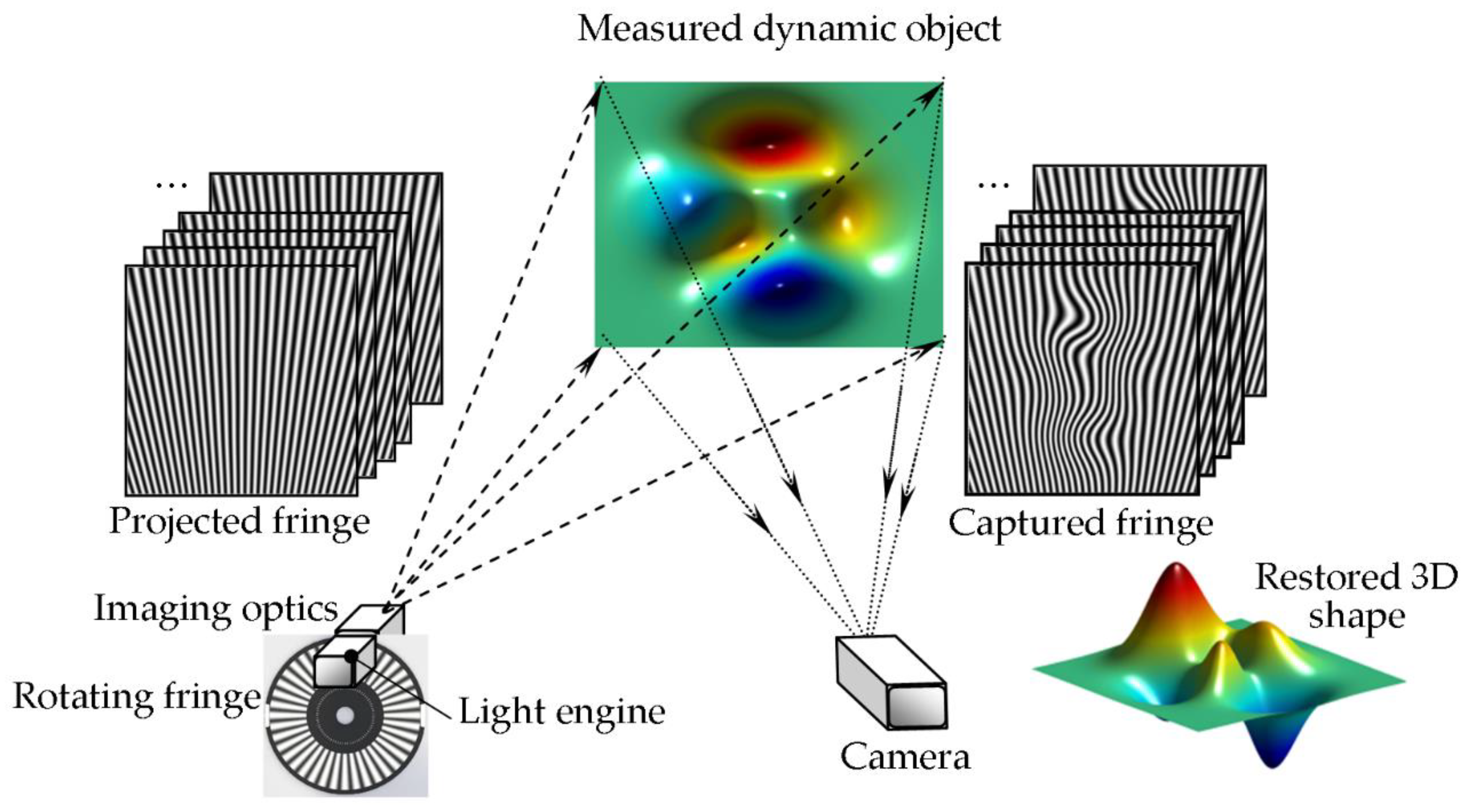
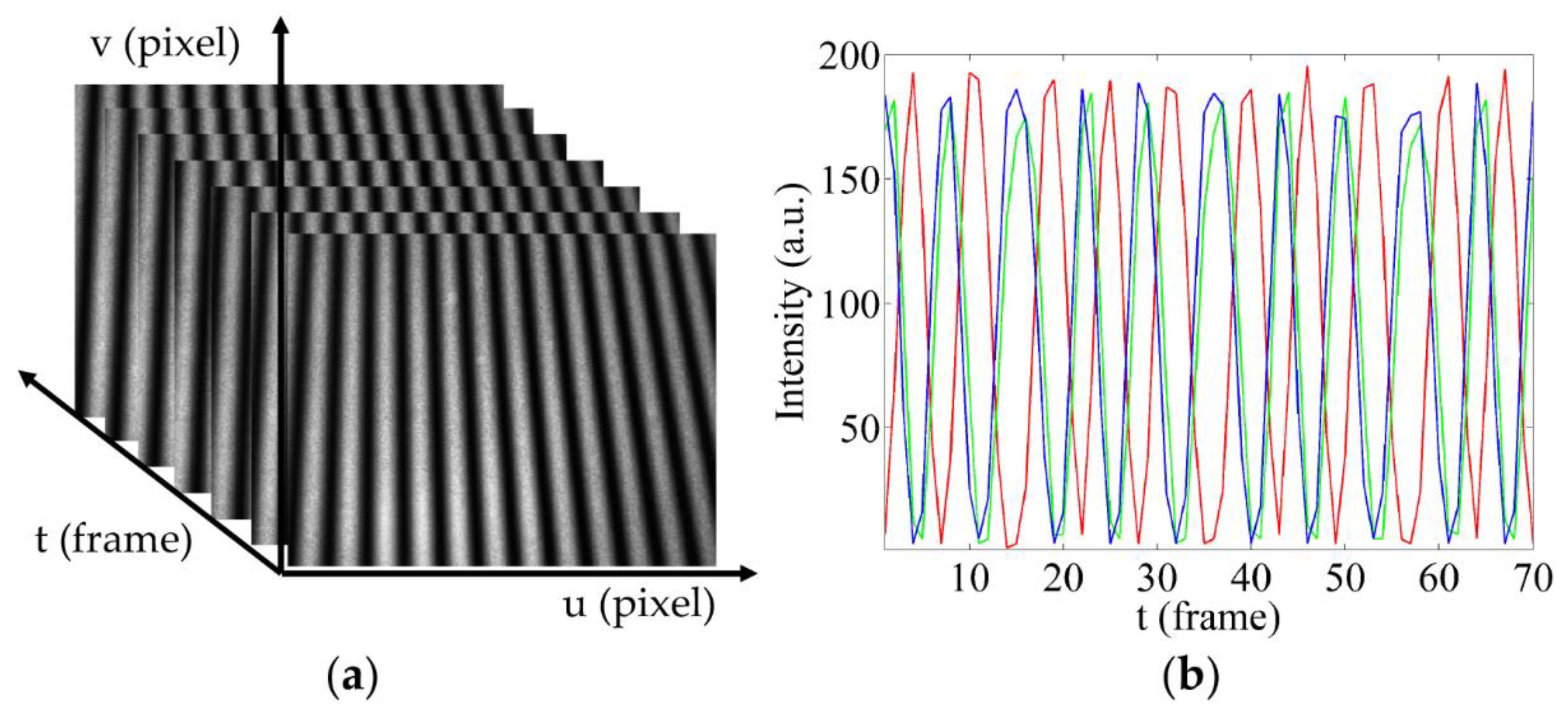
2.1. Principle of TFTP

As is shown in Figure 1, a typical experimental arrangement of TFTP system is similar to that of the FTP system, except for a multi-period phase-shifting projector. The system is mainly composed of a self-made projection device, an imaging device and a dynamic object to be measured. To improve the projection speed of the measuring system, a mechanical projector is employed. Multi-periodic fringe patterns with a fixed phase-shifting interval are generated by the rotating wheel of the mechanical projector and continuously projected onto the surface of the tested object. The fringe pattern is modulated and deformed by the 3D shape of the measured dynamic object. A high-speed camera located on another viewing angle is employed to sample the tested object in the temporal domain and works synchronously with the self-made projector.

At the initial moment t₀, the intensity distribution of fringe pattern can be expressed as

$$I(x,y)=\mathrm{A}(x,y)+\mathrm{B}(x,y)\cos \varphi (x,y),$$

(1)

where (x,y) is the pixel coordinate, A(x,y) is the average intensity, B(x,y) is the intensity modulation, and ϕ(x,y) is the fringe deformation determined by 3D shape of the tested object.

The intensity distribution of the fringe pattern at the moment t can be written as

$$I(x,y,{\delta }_t)=\mathrm{A}(x,y)+\mathrm{B}(x,y)\cos [\varphi (x,y)+{\delta }_{\mathrm{t}}],$$

(2)

where δ_t is the phase modulation introduced by multiple phase shifts during t₀~t.

During the whole dynamic measurement process, n frames of modulated fringe patterns are obtained by sampling the measured object along the temporal axis. As illustrated in Figure 2, a 3D temporal-spatial coordinate system has two spatial coordinates (x,y) and one temporal coordinate (t). It can be seen that the intensity distribution in the temporal domain is an approximate sinusoidal curve, which also carries height information of the measured object. At time t, the intensity distribution along the temporal axis can be represented by

$$g(x,y,t)=a(x,y)+b(x,y)\cos \left[2\pi f_{0}x+\varphi (x,y,t)+2\pi f_{t}t\right],$$

(3)

where a(x,y) is the background intensity, b(x,y) is the intensity modulation, f₀ is the spatial frequency, ϕ(x,y,t) is the phase distribution modulated by the height information of the measured object; 2πf_tt is the phase modulation caused by the multi-period phase-shifting and f_t is the temporal frequency of the phase-shifting.

After the expansion of Equation (3), it can be rewritten as

$$g(x,y,t)=a(x,y)+\frac{b(x,y)}{2}{e}^{i2\pi f_{0}x}{e}^{i\varphi \left(x,y,t\right)}{e}^{i2\pi f_{t}t}+\frac{b(x,y)}{2}{e}^{-i2\pi f_{0}x}{e}^{-i\varphi \left(x,y,t\right)}{e}^{-i2\pi f_{t}t},$$

(4)

As f₀ is the spatial frequency, for any point (x,y), the $e^{i2\pi f_{0}x}$ and $e^{-i2\pi f_{0}x}$ are constant in temporal domain, then Equation (4) can be expressed as

$$g(x,y,t)=a(x,y)+\frac{c(x,y)}{2}{e}^{i\varphi \left(x,y,t\right)}{e}^{i2\pi f_{t}t}+\frac{c^{\prime }(x,y)}{2}{e}^{-i\varphi \left(x,y,t\right)}{e}^{-i2\pi f_{t}t},$$

(5)

It is quite clear that the last two terms of Equation (5) on the spectrum are located on both sides of the zero-frequency component. As is shown in Figure 3, there is no spectral aliasing and the fundamental frequency can be easily filtered out. Inverse Fourier transform operations can be carried out along the temporal axis to obtain the wrapped phase value. The wrapped phase value can be further expressed as

$$\varphi (x,y,t)=phase\left\{F^{-1}\left\{F\left\{\frac{c(x,y)}{2}{e}^{i\varphi \left(x,y,t\right)}{e}^{i2\pi f_{t}t}\right\}\right\}\right\}=\arctan \frac{\mathrm{Im}[\widehat{g}(x,y,t)]}{\mathrm{Re}[\widehat{g}(x,y,t)]},$$

(6)

where $\widehat{g}(x,y,t)=F^{-1}\left\{F\left\{\frac{c(x,y)}{2}{e}^{i\varphi \left(x,y,t\right)}{e}^{i2\pi f_{t}t}\right\}\right\}$, F{#} is the Fourier transform operator, F⁻¹{#} is the inverse Fourier transform operator. The 3D continuous phase distribution can be obtained by,

$$\Phi (x,y,t)=\mathrm{unwrap}\left\{\varphi \left(\mathrm{x},\mathrm{y},\mathrm{t}\right)\right\}-2\pi f_{t}t,$$

(7)

where unwrap{#} is an unwrapping operator. In order to get the natural phase of the measured object, the time modulated factor 2πf_tt should be removed.

The phase to height mapping algorithm [13,14] can be described as

$$\frac{1}{h(u,v,t)}=a_0(u,v)+\frac{a_1(u,v)}{\Delta \Phi (u,v,t)}+\frac{a_2(u,v)}{\Delta {\Phi }^2(u,v,t)}+\frac{a_3(u,v)}{\Delta {\Phi }^3(u,v,t)},$$

(8)

where ∆Φ(u,v,t) is the phase difference of the measured object relative to the reference plane, a₀ … a₃ are equation coefficients. h(u,v,t) is the corresponding height distribution. There are 4 unknown coefficients in Equation (8). Accordingly, at least 5 planes of different height are needed to solve the equation coefficients.

In summary, the flow diagram of the proposed method is described in Figure 4.

2.2. The Measuring Limitation of TFTP

The optical geometry of TFTP is shown in Figure 5, where the optical axis $\overline{P_1{P}_2}$ of the projector crosses that of the camera $\overline{I_1{I}_2}$ at point O on the reference plane, which is perpendicular to $\overline{I_1{I}_2}$. d expresses the distance between P₂ and I₂, and L₀ is the working distance between I₂ and O. Along the temporal axes, $\overline{AC}$ is the distance between points A, C on the reference plane, D expresses a tested point, C and D correspond to the same pixel of the camera at different moments. Assuming the TFTP system is perfect and the system structural parameters d, L₀ are exactly known. The height distribution can be calculated by

$$h(\mathrm{u},v,t)=\frac{\overline{AC}{L}_0}{d+\overline{AC}}=\frac{L_0\Delta \varphi (u,v,t)}{2\pi f_{t}d+\Delta \varphi (u,v,t)},$$

(9)

As the Fourier spectra along the temporal axis usually have multiple components that can be expressed as

$$f_{\mathrm{n}}=n{f}_t+\frac{n}{2\pi }\frac{\partial \varphi (u,v,t)}{\partial t},$$

(10)

In order to obtain the height information accurately, the fundamental component must be separated from all other spectra components, it is necessary that

$$(f_1{)}_{\min }>f_b,$$

(11)

$$(f_1{)}_{\max }<{(f_n)}_{\min },n>1,$$

(12)

where f_b, (f₁)_max represent the maximum frequency of the zero frequency component and the fundamental frequency component respectively. (f₁)_min and (f_n)_min sequentially represent the minimum frequency of the fundamental frequency component and n-order spectral component.

Therefore, the phase variation caused by height modulation should be limited in

$${\left|\frac{\partial \varphi (u,v,t)}{\partial t}\right|}_{\max }<\raisebox{1ex}{$2\pi f_t$}\!\left/ \!\raisebox{-1ex}{$3$}\right.,$$

(13)

As L₀ is much larger than h(u,v,t), Equation (9) can be rewritten as

$$\varphi (u,v,t)\approx \Delta \varphi (u,v,t)=\frac{2\pi f_{t}d}{L_0}h(u,v,t),$$

(14)

Then the height variation should be limited in

$${\left|\frac{\partial h(u,v,t)}{\partial t}\right|}_{\max }<\raisebox{1ex}{$L_0$}\!\left/ \!\raisebox{-1ex}{$3d$}\right.,$$

(15)

During the measurement process, if the height variation along the temporal axis exceeds the limitation, the fundamental components would overlap the zero component and other components in their Fourier spectrum domain. If this occurs, the tested object’s shape at that moment cannot be restored correctly.

In Reference [6], because of the discrete nature of discrete Fourier transform (DFT), Su et al. proposed the relationship between the sampling frequency m and the frequency spectra orders n of the adjacent frequency period.

$$m\ge \frac{4}{3}\left(n+1\right),n\ge 2,$$

(16)

Consequently, in case of sinusoidal fringe pattern projection, at least four sampling points were required to avoid spectral overlapping.

For the convenience of data processing, a serial of sinusoidal periodic signals—five sampling points per period (T = 5)—was simulated. Considering the length of time that the dynamic object lasted, the appropriate sampling rate of the employed high-speed camera was selected to capture as many frames of deformed fringe patterns as possible. To ensure temporal resolution and measuring accuracy, multiple periodic signals were constructed to analyze the phase variation along the temporal axis with TFTP. During the following computer simulation and dynamic measurement process, 201 and 630 frames of images were captured along the temporal axis respectively. This suggests that the presented TFTP method is especially suitable for multi-frame 3D shape measurement of a complex dynamic object which cannot be successfully digitalized by traditional FTP in 2D spatial fringe analysis.

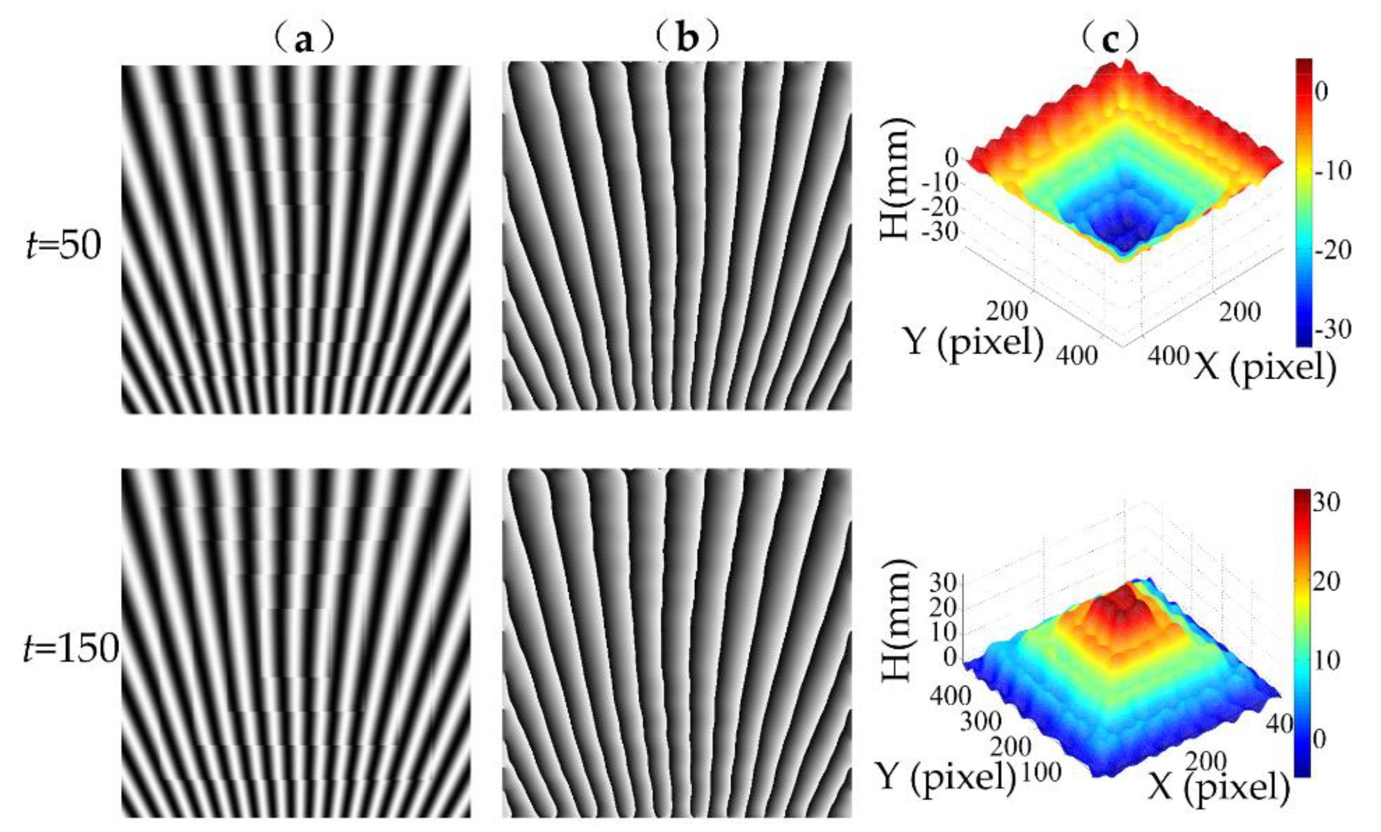
3. Computer Simulation

The working process of TFTP system was simulated. The angle between the optical axis of CCD and that of the projection device was set to 25°. As is shown in Figure 6, a moving stepped model that clearly contains high-frequency components was designed for dynamic measurement. The lateral size of the stepped model was 512 × 512 pixels, and its height varied from −60 mm to 60 mm. Radial fringes with a fixed phase-shifting interval were sequentially projected onto the surface of the measured object and 201 sampling moments of the dynamic measurement were simulated. The selected starting point of the temporal phase unwrapping was t₀ = 100.

When the dynamic stepped model was measured by the conventional FTP method in 2D spatial domain, the details of the step’s edge would be smoothed due to the spatial weighted filtering operation. The corresponding reconstruction results of two different moments are illustrated in Figure 7.

When the same dynamic model was measured by TFTP, the reconstructed results of t = 50, 150, as shown in Figure 8, demonstrate that the proposed method can effectively retain the high-frequency spatial components of the measured object, i.e., the details of the stepped model’s edge. This benefits from none weighted filtering operations in 2D spatial spectrum while the deformed fringes processing by TFTP along the temporal domain.

4. Experimental Results

The actual projection system is shown in Figure 9. The radiated Rochi grating was equally produced on a film. A Kohler illumination system was adopted to homogenize the projector’s lighting source. Multi-period fringe patterns with a fixed phase-shifting interval were continuously projected onto the surface of a tested object by the wheel rotating at 600 rpm. A series of trigger pulse was generated by detecting the marking points on the film to trigger the camera (Mars 800-545 um) located at another viewing angle. The synchronization between the projector and the camera was realized. The intensity distribution was integrated dynamically through exposure. A sequence of fringe patterns captured by the camera is illustrated in Figure 10a. The intensity distribution along the temporal axis is shown in Figure 10b.

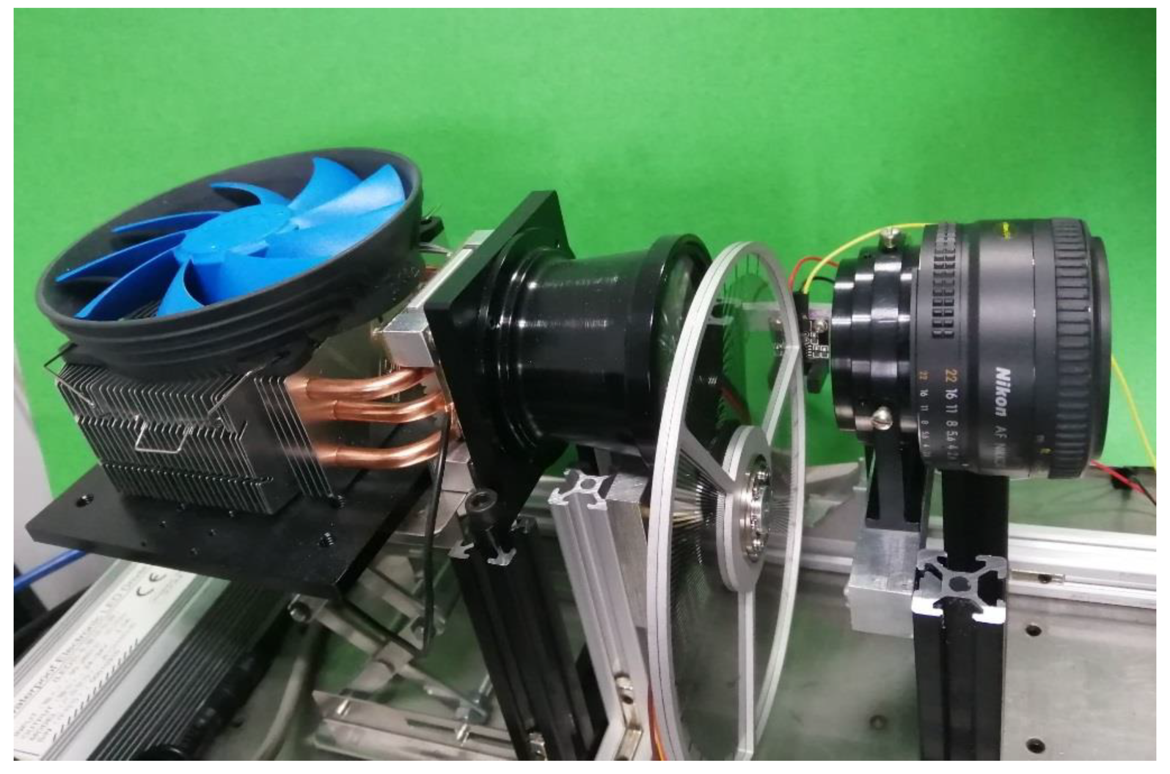
4.1. System Calibration

As shown in Figure 11a, a standard block was designed to calibrate the TFTP system. There are six standard cylinders located evenly on a plane. Each standard cylinder consists of four cylinders with different heights and diameters. The distance between adjacent parallel planes is 150 mm, 200 mm, 200 mm and 250 mm. A slope connecting two adjacent parallel planes was designed to ensure the continuity of the phase distribution between planes with different heights. One of the deformed fringe patterns is shown in Figure 11b. FFT, band-pass filtering and inverse transform operations were performed along the temporal axis pixel by pixel. The corresponding wrapped phase is shown in Figure 11c. The moment t₀ = 8 was selected as the initial moment. The wrapped phase of the standard block was unwrapped and guided by its modulation distribution [15]. The corresponding unwrapped phase distribution is shown in Figure 11d.

Phase distribution with the same height but in six different locations was extracted to fit a ternary cubic surface by least squares method. Then the phase distributions of five different heights were fitted. By defining one plane as the reference plane, the distances between the other four planes and the reference plane were known. Finally, with the calculated phase difference relative to the reference plane and substituting the phase difference into Equation (8), the height-to-phase mapping coefficients can be obtained to recover the 3D shape of the tested object.

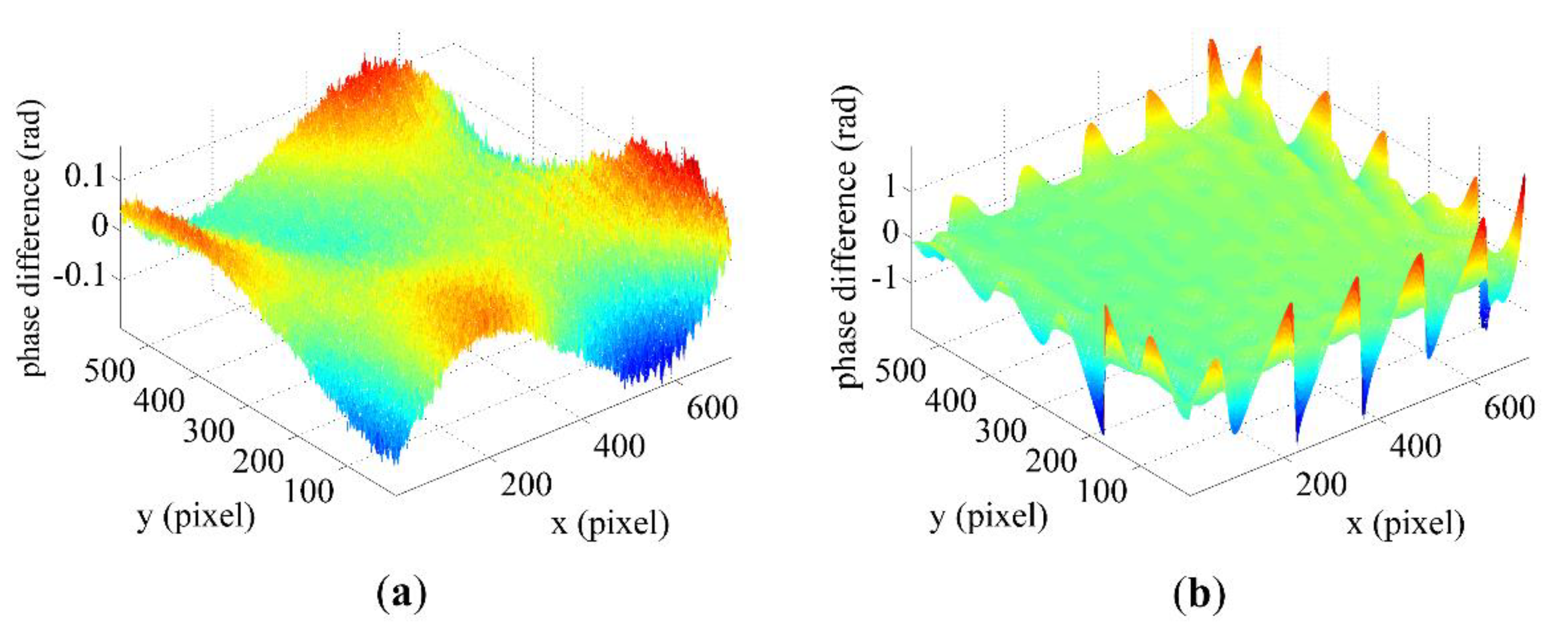
4.2. Accuracy Evaluation of TFTP

To quantify the accuracy of this TFTP system, a standard plane was measured. The reconstructed phase difference is shown in Figure 12a, at the moment t₀ = 8, the root mean squared error (RMSE) of the phase distribution is 0.0380 rad, and that of height reconstruction is 0.0794 mm.

As shown in Figure 12b, when the same plane is measured by the traditional FTP it is impossible to realize integer period sampling because the measurement error of the edge parts is extremely large. The RMSE of the phase distribution is 1.1792 rad and that of height distribution is 6.3815 mm.

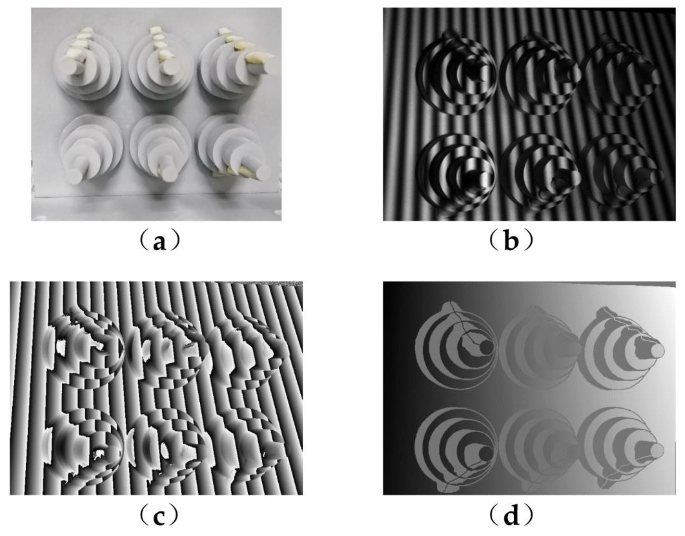
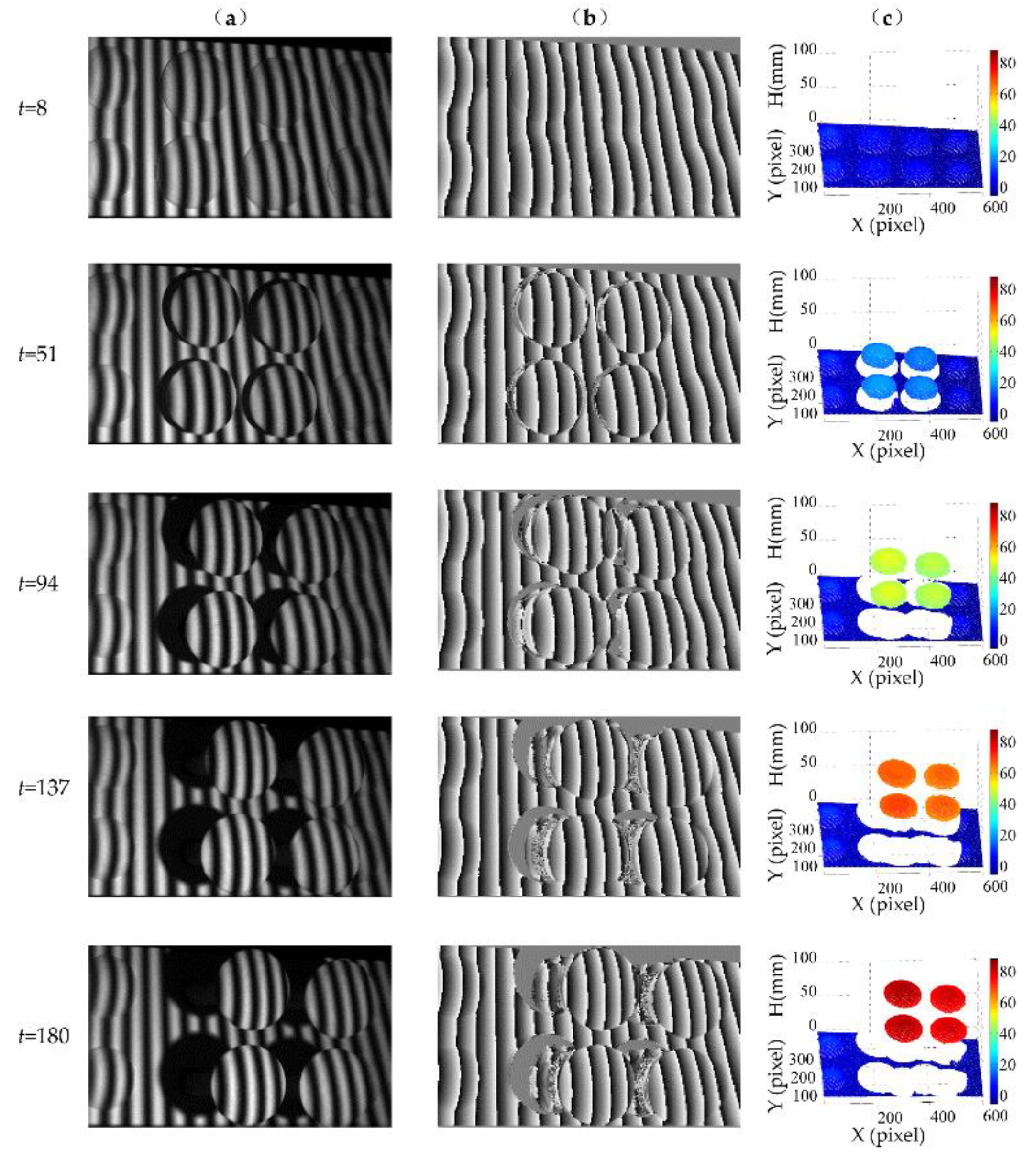
4.3. Dynamic Measurement

As shown in Figure 13, a wooden movable model was chosen as the tested object. There are four circular buckles of 33 mm in diameter fixed on the model. The movable part consists of four buckles of 39 mm in diameter which can be manually pushed out and pulled back.

Throughout the measurement, 630 frames of deformed fringe patterns had been captured. The moment t₀ = 8 was selected as the initial moment whose wrapped phase can be successfully unwrapped in 2D spatial domain. Then, the unwrapped, continuous and natural phase value on each pixel of the initial moment were taken as the starting point, from which the 3D wrapped phase values were unwrapped along the temporal axis pixel by pixel. The moments t = 8, 51, 94, 137, 180 are taken as examples. The deformed fringe patterns, corresponding wrapped phase distribution and 3D reconstruction of five different moments are illustrated in Figure 14a–c, respectively.

Throughout the entire reconstruction process, the phase value of each pixel was calculated independently along the temporal axis. This method successfully maintained the idea that every single deformed fringe pattern corresponded to one 3D reconstruction result. The experimental results show that TFTP can be applicable for measuring the isolated dynamic object.

5. Discussion and Conclusions

When a conventional phase-shifting method is employed in measuring dynamic scene, three images can determine the phase. In this method, only one corresponding phase can be determined by each group of three images. It is an average effect in a short period of time during the acquisition of the three images. The accuracy of the measurement result is also affected by motion blur. In consideration of the dynamic object’s moving nature, appropriate sampling rate of the employed high-speed camera should be selected to capture as many frames of deformed fringe patterns as possible. Then, to ensure temporal resolution and measuring accuracy, multiple periodic signals are constructed to analyze the phase variation along temporal axis with TFTP. In the proposed method, only one frame of the deformed fringe pattern is required to calculate its corresponding phase distribution and it is only limited by the sampling rate of the employed high-speed camera.

During the measurement process, when the dynamic object moves both in the horizontal or vertical direction at the same time, the 3D reconstruction can also be retrieved. If it moves much faster, guaranteeing successful reconstruction and improving measurement accuracy can be achieved by having the negative influence reduced. This is done by decreasing the spatial frequency of the projected fringe pattern or accelerating the sampling speed along the temporal axis. If the dynamic object is broken after fracture, the 3D shape of measurement object can also be reconstructed as long as the sampling rate of the employed high-speed camera is fast enough to ensure the phase distribution is continuous along the temporal axis.

As a novel 3D shape measurement profilometry, TFTP only performs Fourier transform, band-pass filtering, and inverse Fourier transform operations along the temporal axis pixel by pixel and never performs weighted filtering operation in spatial domain. The high-frequency spatial components of the tested isolated dynamic object have been successfully retained. TFTP neither limits to precise phase-shifting techniques, nor does it require strict spatial modulation frequencies. During the whole measurement process for dynamic object, only one 2D wrapped phase is required to be correctly unwrapped in spatial domain, and the whole 3D wrapped phase can be easily unwrapped via temporal axis. This method essentially requires one single deformed fringe pattern to retrieve its corresponding 3D shape of the measured dynamic object, and is only limited by the sampling rate of the employed high-speed camera. This possesses an obvious advantage for high speed measurement of dynamic process. The current recording speed is 300fps, which can be raised if the marking points on the film are increased or the recording rate of the employed camera is faster.

References

1. Gorthi, S.S.; Rastogi, P. Fringe projection techniques: Whither we are? Opt. Laser Eng. 2010, 48, 133–140. [Google Scholar] [CrossRef]
2. Chen, F.; Brown, G.; Song, M. Overview of three-dimensional shape measurement using optical methods. Opt. Eng. 2000, 39, 10–22. [Google Scholar]
3. Halioua, M.; Liu, H.C. Optical three-dimensional sensing by phase measurement profilometry. Opt. Laser Eng. 1989, 11, 185–215. [Google Scholar] [CrossRef]
4. Zuo, C.; Feng, S.J.; Huang, L.; Tao, T.Y.; Yin, W.; Chen, Q. Phase shifting algorithms for fringe projection profilometry: A review. Opt. Laser Eng. 2018, 109, 23–59. [Google Scholar] [CrossRef]
5. Takeda, M.; Mutoh, K. Fourier Transform Profilometry for the auto measurement of 3-D object shapes. Appl. Opt. 1983, 22, 3977–3982. [Google Scholar] [CrossRef] [PubMed]
6. Su, X.Y.; Chen, W.J. Fourier transform profilometry: A review. Opt. Laser Eng. 2001, 35, 263–284. [Google Scholar] [CrossRef]
7. Su, X.Y.; Zhang, Q.C. Dynamic 3D shape measurement method: A review. Opt. Laser Eng. 2010, 48, 191–204. [Google Scholar] [CrossRef]
8. Wissmann, P.; Forster, F.; Schmitt, R. Fast and low-cost structured light pattern sequence projection. Opt. Express 2011, 19, 24657–24671. [Google Scholar] [CrossRef] [PubMed]
9. Heist, S.; Mann, A.; Kühmstedt, P.; Schreiber, P.; Notni, G. Array projection of aperiodic sinusoidal fringes for high-speed three-dimensional shape measurement. Opt. Eng. 2014, 53, 112208. [Google Scholar] [CrossRef]
10. Heist, S.; Lutzke, P.; Schmidt, I.; Dietrich, P.; Kühmstedt, P.; Tünnermann, A.; Notni, G. High-speed three-dimensional shape measurement using GoBo projection. Opt. Laser Eng. 2016, 87, 90–96. [Google Scholar] [CrossRef]
11. Hyun, J.; Chiu, G.; Zhang, S. High-speed and high-accuracy 3D surface measurement using a mechanical projector. Opt. Express 2018, 26, 1474–1487. [Google Scholar] [CrossRef] [PubMed]
12. Zhang, S. High-speed 3D shape measurement with structured light methods: A review. Opt. Laser Eng. 2018, 106, 119–131. [Google Scholar] [CrossRef]
13. Zhou, W.S.; Su, X.Y. A Direct Mapping Algorithm for Phase-measuring Profilometry. J. Mod. Opt. 1994, 41, 89–94. [Google Scholar] [CrossRef]
14. Su, X.Y.; Song, W.Z.; Cao, Y.P.; Xiang, L.Q. Phase-height mapping and coordinate calibration simultaneously in phase-measuring profilometry. Opt. Eng. 2004, 43, 708–712. [Google Scholar]
15. Su, X.Y.; Chen, W.J. Reliability-guided phase unwrapping algorithm: A review. Opt. Laser Eng. 2004, 42, 245–261. [Google Scholar] [CrossRef]
Figure 1. Schematic diagram of a typical temporal Fourier transform profilometry (TFTP) setup.
Applsci 09 04123 g001
Figure 2. Temporal intensity distribution of the same pixel in n frames phase-shifting deformed images.
Applsci 09 04123 g002
Figure 3. Spectrum distribution of each pixel along the temporal axis.
Applsci 09 04123 g003
Figure 4. Flow diagram of this proposed method.
Applsci 09 04123 g004
Figure 5. Optical geometry.
Applsci 09 04123 g005
Figure 6. Simulated dynamic stepped model at different moments (a) t = 50 (b) t = 100 (c) t = 150.
Applsci 09 04123 g006
Figure 7. Simulation results of two different moments by conventional FTP. (a) Deformed fringe patterns. (b) Wrapped phase and (c) 3D reconstruction.
Applsci 09 04123 g007
Figure 8. Simulation results of 2 different moments by TFTP. (a) Wrapped phase. (b) 3D reconstruction.
Applsci 09 04123 g008
Figure 9. Experimental setup.
Applsci 09 04123 g009
Figure 10. Deformed fringe patterns. (a) A sequence of deformed fringe pattern captured by the camera. (b) Intensity distribution along the temporal axis.
Applsci 09 04123 g010
Figure 11. System calibration process: (a) standard block. (b) deformed fringe pattern on block captured by the camera, (c) wrapped phase distribution calculated by TFTP, (d) unwrapped phase distribution.
Applsci 09 04123 g011
Figure 12. Reconstructed phase difference distribution of the tested standard plane by (a) TFTP and (b) traditional FTP.
Applsci 09 04123 g012
Figure 13. Tested object whose circular buckles can be manually pushed out and pulled back.
Applsci 09 04123 g013
Figure 14. Experimental results of a moving wooden model. (a) Deformed fringe patterns, (b) wrapped phase distribution and (c) 3D reconstruction of 5 different moments.
Applsci 09 04123 g014