Hydrodynamic Ram Effect Caused by Debris Hypervelocity Impact on Satellite Tank

Abstract
Featured Application
Abstract
1. Introduction
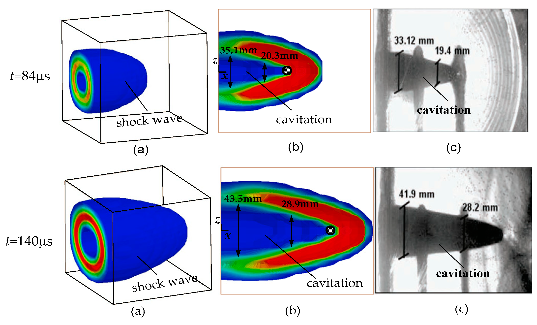
2. Validation of Simulation Model
3. Numerical Simulation of the Debris Impact on Satellite Tank
3.1. Simulation Model of the Debris Impacting Satellite Tank
3.2. Velocity Attenuation of Debris
3.3. Shock Wave Propagation
3.4. Perforation of Front and Back Walls
4. Influence of Liquid-Filling Ratio on Hydrodynamic Ram Effect
4.1. Simulation Modes with Different Liquid-Filling Ratios
4.2. Perforation and Stress on Front and Back Walls
5. Influence of Angular Velocity on Hydrodynamic Ram Effect
5.1. Influence of Angular Velocity Direction on Hydrodynamic Ram Effect
5.2. Influence of Angular Velocity Magnitude on the Hydrodynamic Ram Effect
6. Conclusions
- When the debris impacted the satellite tank at the velocity of 7000 m/s, it passed through the tank at t = 1196 μs, and the residual velocity was 263 m/s, indicating that the debris velocity was significantly reduced by the hydrodynamic ram effect.
- The shock wave pressure on the front wall was the highest, which exceeded the yield strength of titanium, so perforations and bulges occurred. Except for the front wall, the pressure on the tank walls was smaller than the yield strength of titanium. Under the action of debris penetration and high pressure hydrazine, perforations and bulges also occurred on the back wall. In the structural design of the satellite tanks, the material strength of the walls should be increased as much as possible, and the protection should be strengthened in vulnerable areas.
- With the reduction in the liquid-filling ratios, the damage caused by the hydrodynamic ram effect weakened and the satellite tank fully-filled with liquid hydrazine was the most severely damaged.
- When the debris impacted the satellite tank with the angular velocities in the x direction, the debris trajectory did not deflect. When the debris impacted the satellite tank with the angular velocities in the y and z direction, the debris trajectory deflected to the negative direction of the z axis and y axis under the action of the Magnus force.
- There was a steady angular velocity in the x direction. Under the steady angular velocity, the damage to the tank was the most serious. With the increase in the angular velocity in the y and z direction, the damage to the tank became more serious.
Author Contributions
Funding
Acknowledgments
Conflicts of Interest
References
- Shen, H.R.; Wang, W.J.; Li, Y.Y.; Shao, Q.L. Modeling and Analysis of Spacecraft Impact; Science Press: Beijing, China, 2014; p. 138. [Google Scholar]
- Varas, D.; Lopez-piente, J.; Zaera, R. Numerical analysis of the hydrodynamic ram phenomenon in aircraft fuel tanks. AIAA J. 2012, 50, 1621–1630. [Google Scholar] [CrossRef]
- Han, L.; Han, Q.; Yang, S. Simulation analysis of hydrodynamic ram in an aircraft fuel tank subjected to high-velocity muti-fragment impact. Explos. Shock Waves 2018, 38, 473–484. [Google Scholar]
- Xu, S.X.; Wu, W.G.; Li, X.B.; Kong, X.S.; Huang, Y.L. Protective effect of guarding fluid cabin bulkhead under attacking by explosion fragment. Explos. Shock Waves 2010, 30, 395–400. [Google Scholar]
- Varas, D.; Zaera, R.; Lopz-Puente, J. Numerical modelling of the hydrodynamic ram phenomenon. Int. J. Impact Eng. 2009, 36, 363–374. [Google Scholar] [CrossRef]
- Disimile, P.J.; Swanson, L.A.; Toy, N. The hydrodynamic ram pressure generated by spherical projectiles. Int. J. Impact Eng. 2009, 36, 821–829. [Google Scholar] [CrossRef]
- Townsend, D.; Park, N.; Devall, P.M. Failure of fluid filled structures due to high velocity fragment impact. Int. J. Impact Eng. 2003, 29, 723–733. [Google Scholar] [CrossRef]
- Nishida, M.; Tanaka, K. Experimental study of perforation and cracking of water-filled aluminum tubes impacted by steel spheres. Int. J. Impact Eng. 2006, 32, 2000–2016. [Google Scholar] [CrossRef]
- Varas, D.; Lopez-piente, J.; Zaera, R. Experimental analysis of fluid-filled aluminium tubes subjected to high-velocity impact. Int. J. Impact Eng. 2009, 36, 81–91. [Google Scholar] [CrossRef]
- Ma, L.Y.; Li, X.D.; Zhou, L.W.; Zhang, G.F. Study on the characteristics of cavity formed by fragment impacting liquid filling container. Explos. Shock Waves 2018, 38, 235–241. [Google Scholar]
- Kong, X.S.; Wu, W.G.; Li, J.; Li, X.B.; Xu, S.X. Effects of explosion fragments penetrating defensive liquid-filled cabins. Explos. Shock Waves 2013, 33, 471–478. [Google Scholar]
- Aziz, M.R.; Kuntjoro, W.; David, N.V. Pressure history in hydrodynamic Ram (HARM) by using FEM-SPH approach. In Proceedings of the 6th International Conference on Control System, Computing and Engineering IEEE, Penang, Malaysia, 25–27 November 2016; pp. 108–112. [Google Scholar]
- Kangjie, R.Y. Simulation of Hydrodynamic Ram Phenomenon Using MSC Dytran; Nanyang Technological University: Singapore, 2008. [Google Scholar]
- Varas, D.; Zaera, R.; Lopz-Puente, J. Numerical modelling of partially filled aircraft fuel tanks submitted to hydrodynamic ram. Aerosp. Sci. Technol. 2012, 16, 19–28. [Google Scholar] [CrossRef]
- Han, L.; Han, Q.; Yang, S. Simulation analysis of hydrodynamic ram factors and effects in aircraft fuel tank. Adv. Aeronaut. Sci. Eng. 2018, 9, 490–500. [Google Scholar]
- Rucker, M.A.; Beeson, H.; Stoltzfus, J.M.; Frank, J.B. Demonstration of Hazardous Hypervelocity Test Capability; Report TR-692-001; White Sands Test Facility: Las Cruces, NM, USA, 1991. [Google Scholar]
- Wilson, C.W.; Warne, D.; Chatfield, M.D. Fuel Tank Explosion Lethality; Report 91-5425-SH; Science Applications International Corporation: Reston, VA, USA, 1991. [Google Scholar]
- Martin, L.; Michel, A.; Chiara, B.; Doormaal, J.C.A.M.; Christof, H.; Gotz, H.; Oliver, M.; Arja, S.; George, S.; Laurent, T.; et al. Design of Blast-Loaded Glazing Windows and Facades: A Review of Essential Requirements towards Standardization. Adv. Civ. Eng. 2016, 2016, 2604232. [Google Scholar]
- Zhang, K.F.; Liang, M.Z.; Lu, F.Y.; Li, X.Y. Mechanics of plate fracture from detonation wave interaction. Propell. Explos. Pyrot. 2019, 44, 188. [Google Scholar] [CrossRef]
- Garcia, B.O.; Chavez, D.J. Shock compression of liquid hydrazine. In Proceedings of the 1995 Shock Compression Conference, Seattle, WA, USA, 15–18 August 1995. [Google Scholar]
- Li, Y.F.; Jin, Q.C.; Liu, Z.D.; Li, G. Finite element analysis of a propellant satellite tank based on ANSYS. Aerosp. Manuf. Technol. 2012, 12, 10–15. [Google Scholar]
- Lecysyn, N.; Bony, D.A.; Aprin, L.; Heymes, F.; Slangen, P.; Dusserre, G.; Munier, L.; Gallic, C.L. Experimental study of hydraulic ram effects on a liquid storage tank: Analysis of overpressure and cavitation induced by a high-speed projectile. J. Hazard. Mater. 2010, 178, 635–643. [Google Scholar] [CrossRef] [PubMed]
- Munson, B.R.; Young, D.F.; Okiishi, T.H.; Huebsch, W.W. Fundamentals of Fluid Mechanics, 6th ed.; Wiley: Hoboken, NJ, USA, 2009; pp. 500–503. [Google Scholar]
- Lei, J.M.; Li, T.T.; Huang, C. A numerical investigation of Magnus effect for high-speed spinning projectile. Acta Armam 2013, 34, 718–725. [Google Scholar]
- Gu, J.N.; Zhang, Z.H.; Fan, W.J. Experimental study on the penetration law for a rotating pellet entering water. Explos. Shock Waves 2005, 25, 341–349. [Google Scholar]


| Material | ρ (kg/m3) | S1 | S2 | S3 | γ0 | C4 | C5 |
|---|---|---|---|---|---|---|---|
| Water | 1000 | 1.979 | 0 | 0 | 0.11 | — | — |
| Air | 1.29 | — | — | — | — | 0.4 | 0.4 |
| Material | ρ (kg/m3) | A (MPa) | B (MPa) | n | C | m |
|---|---|---|---|---|---|---|
| Aluminum | 2700 | 200 | 144 | 0.62 | 0.01 | 1.00 |
| Steel | 7830 | 496 | 434 | 0.307 | 0.008 | 0.804 |
| t (μs) | x (cm) | ds (mm) | de (mm) | ε/% |
|---|---|---|---|---|
| 84 | 1.5 | 35.1 | 33.12 | 5.9 |
| 5.0 | 20.3 | 19.4 | 4.6 | |
| 140 | 2.0 | 43.5 | 41.9 | 3.8 |
| 7.5 | 28.9 | 28.2 | 2.5 |
| Material | ρ (kg/m3) | Cl (m/s) | S1 | S2 | S3 | γ0 |
|---|---|---|---|---|---|---|
| Liquid hydrazine | 1008 | 1500 | 1.979 | — | — | 0.11 |
| Material | ρ (kg/m3) | E (GPa) | υ | σs (MPa) | σb (MPa) |
|---|---|---|---|---|---|
| Titanium | 4500 | 118 | 0.34 | 820 | 890 |
| Deformation (cm) | 100% | 90% | 80% | 70% |
|---|---|---|---|---|
| Diameter of front perforation | 10.23 | 9.46 | 9.20 | 9.08 |
| Diameter of back perforation | 6.90 | 6.24 | 5.51 | 5.05 |
| Bulge height on front wall | 1.12 | 0.99 | 0.79 | 0.71 |
| Bulge height on back wall | 1.58 | 1.45 | 1.33 | 1.29 |
© 2019 by the authors. Licensee MDPI, Basel, Switzerland. This article is an open access article distributed under the terms and conditions of the Creative Commons Attribution (CC BY) license (http://creativecommons.org/licenses/by/4.0/).
Share and Cite
Zhao, B.; Zhao, J.; Cui, C.; Duan, Y. Hydrodynamic Ram Effect Caused by Debris Hypervelocity Impact on Satellite Tank. Appl. Sci. 2019, 9, 4200. https://doi.org/10.3390/app9204200
Zhao B, Zhao J, Cui C, Duan Y. Hydrodynamic Ram Effect Caused by Debris Hypervelocity Impact on Satellite Tank. Applied Sciences. 2019; 9(20):4200. https://doi.org/10.3390/app9204200
Chicago/Turabian StyleZhao, Beilei, Jiguang Zhao, Cunyan Cui, and Yongsheng Duan. 2019. "Hydrodynamic Ram Effect Caused by Debris Hypervelocity Impact on Satellite Tank" Applied Sciences 9, no. 20: 4200. https://doi.org/10.3390/app9204200
APA StyleZhao, B., Zhao, J., Cui, C., & Duan, Y. (2019). Hydrodynamic Ram Effect Caused by Debris Hypervelocity Impact on Satellite Tank. Applied Sciences, 9(20), 4200. https://doi.org/10.3390/app9204200