Abstract
In recent years, machine learning methods have shown the great potential for real-time transient stability status prediction (TSSP) application. However, most existing studies overlook the imbalanced data problem in TSSP. To address this issue, a novel data segmentation-based ensemble classification (DSEC) method for TSSP is proposed in this paper. Firstly, the effects of the imbalanced data problem on the decision boundary and classification performance of TSSP are investigated in detail. Then, a three-step DSEC method is presented. In the first step, the data segmentation strategy is utilized for dividing the stable samples into multiple non-overlapping stable subsets, ensuring that the samples in each stable subset are not more than the unstable ones, then each stable subset is combined with the unstable set into a training subset. For the second step, an AdaBoost classifier is built based on each training subset. In the final step, decision values from each AdaBoost classifier are aggregated for determining the transient stability status. The experiments are conducted on the Northeast Power Coordinating Council 140-bus system and the simulation results indicate that the proposed approach can significantly improve the classification performance of TSSP with imbalanced data.
1. Introduction
With the emergence of the large-scale interconnected power grid and the high penetration of distributed generation, modern power systems are faced with severe challenges for stable operation. Transient stability is a crucial and complex issue in modern power systems [1]. Rapid and accurate recognition of transient stability status is important for being aware of the imminent unstable risk so that enough time is available for applying the appropriate control strategies to prevent catastrophic outage [2].
Classical transient stability analysis methods can be categorized into two branches, time-domain simulation (TDS) and transient energy function (TEF) [3,4]. Although the TDS method is straightforward and reliable, its high time complexity hinders real-time decision-making applications. As for the TEF method, it has low computational cost and provides the transient stability margin, but it is normally difficult to construct an available energy function when considering detailed system models.
With the wide deployment of phasor measurement unit devices, tremendous synchrophasor data is accessible for monitoring the stability of power systems [5]. As a key tool for power system data analysis, machine learning shows great potential for real-time transient stability status prediction (TSSP) applications. Generally, TSSP itself can be regarded as a binary classification problem [6], i.e., stable/unstable status. In the offline, the nonlinear relationship between the selected features and the corresponding stability status can be established via machine learning methods. When online, transient stability status can be predicted immediately after feeding the collected features to the classification model. Up to now, a variety of machine learning methods have been applied for TSSP, e.g., neural networks [7,8], support vector machines [9,10], decision trees [11], and ensemble learning [12,13].
In general, practical power systems can remain at transient stable status when subjected to most disturbances. That is to say, an unstable status is detected only in a few situations, which results in the imbalanced data problem in the training database, i.e., stable samples significantly outnumber unstable samples [14,15]. Faced with this issue, conventional machine learning methods aiming to minimize the overall error rate tend to classify the samples as the stable class and show ineffectiveness in identifying unstable samples [14]. It is known that the unstable class is more important than the stable class for power system operators, and poor recognition of unstable samples would dramatically deteriorate the practical utility of the TSSP classification model.
In the machine learning community, the imbalanced data problem in classification tasks is a hot topic of research and effective solutions can mainly be divided into data-level and algorithm-level approaches [16]. The former achieves data rebalance by adding samples of minority class, namely oversampling, or reducing samples of majority class, namely undersampling. The latter handles this problem via enhanced classification algorithms, e.g., cost-sensitive learning [17,18].
However, few studies attempted to counteract the negative effects of imbalanced data for TSSP. Specifically, the unstable samples are duplicated to balance the sample number of different classes in Reference [14]. Although this method could be simply and directly conducted, it is prone to overfitting [18]. An adaptive synthetic sampling (ADASYN) algorithm is adopted in Reference [15] to generate more unstable samples, but the generated unstable samples by linear interpolation are hard related to the actual operating conditions of power systems, which may affect the rationality of the classification model.
In this paper, a novel data segmentation-based ensemble classification (DSEC) method is proposed to better handle the imbalanced data problem of TSSP. The DSEC method consists of three steps. In the first step, the data segmentation strategy is utilized for dividing the stable samples into multiple non-overlapping stable subsets, ensuring that the samples in each stable subset are not more than the total unstable ones, then each stable subset is combined with the unstable set to form a training subset. For the second step, an AdaBoost classifier is constructed based on each training subset. In the final step, decision values from each AdaBoost classifier are aggregated for determining the transient stability status.
The rest of this paper is organized as follows: Section 2 investigates the effects of the imbalanced data problem on TSSP. The DSEC method is proposed in Section 3. The TSSP based on the DSEC method is introduced in Section 4. The case studies are shown in Section 5. Finally, conclusions are drawn in Section 6.
2. Effects of the Imbalanced Data Problem on TSSP
2.1. The Breif Description of the TSSP Issue
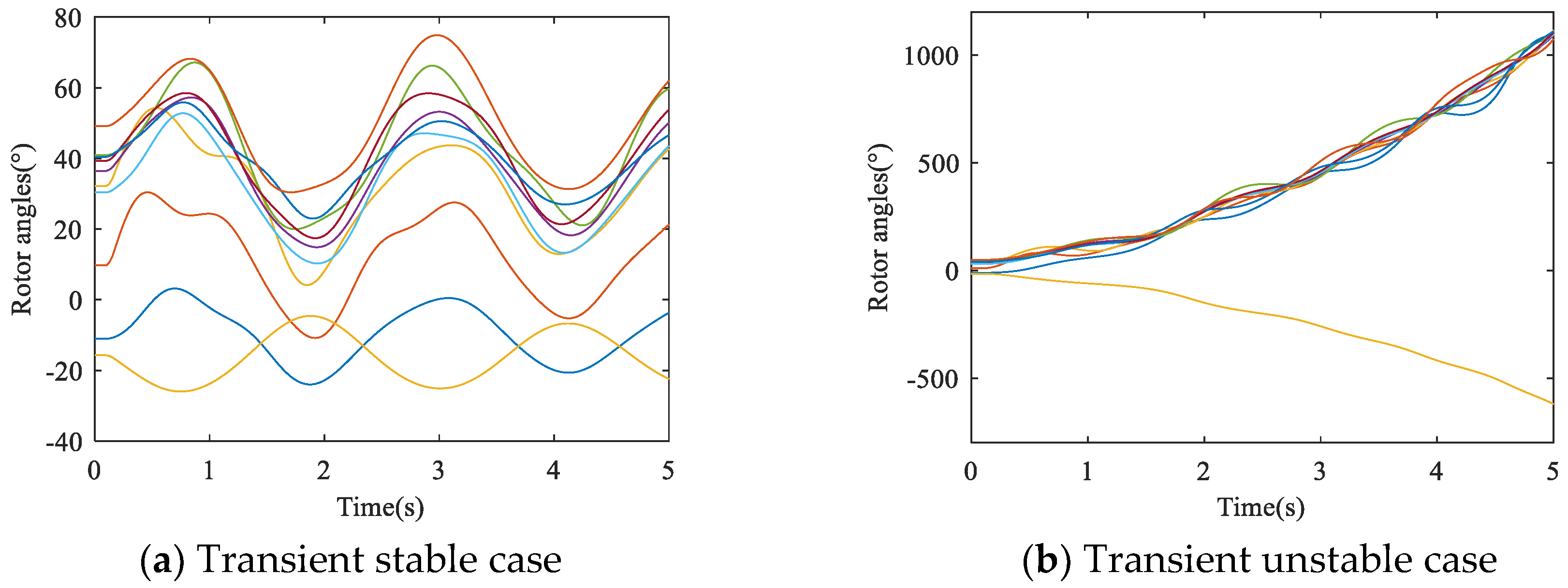
Transient stability refers to the ability of the power system to maintain synchronism after large disturbances, and it is mainly affected by the operating condition and the fault condition [1]. When using the TDS method for transient stability analysis, the stability status of the power system is usually determined by whether the rotor angle of any generator is greater than 360° or not at the end of the simulation time [6]. If all rotor angles of generators are less than 360°, the power system is considered transient stable, otherwise, it is transient unstable. For illustration, a three-phase short-circuit fault occurs at the head of line 8–9 in the IEEE 39-bus system. Figure 1 shows the rotor angle curves corresponding to different time of faults duration. In this figure, (a) represents the transient stable case when fault duration is set to 0.1 s and (b) represents the unstable case when fault duration is set to 0.26 s. As the transient unstable process works so fast, an accurate and rapid method for TSSP is urgently needed to avoid blackout and to provide the auxiliary decision support for operators.
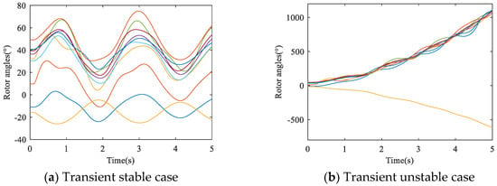
Figure 1.
Illustration of transient stable and unstable cases.
2.2. The Effect on the Decision Boundary
The TSSP based on machine learning methods can be regarded as a binary classification problem and the decision boundary between stable and unstable classes is built by the classification method in the feature space. Given the training set D= {(x1, y1), (x2, y2), …, (xN, yN)}, yi ∈ {−1,1}, the loss function of the machine learning method is generally expressed as follows:
where xi represents the feature vector of sample i and yi is the corresponding class label. Here, if yi = 1, it is unstable; otherwise, it is stable. The value N is the number of training samples. The value f represents the decision function. The I is indication function and if its internal logic is true, the value is 1; otherwise, it returns 0.
For transient stability status classification problem, training set D can be divided into the stable set DS and the unstable set DU, and Equation (1) can be further expressed as follows:
where εS and εU are the classification error rates of stable class and unstable class, respectively, and NS and NU are the number of stable samples and unstable samples in the training set, respectively.
From Equation (2), it can be seen that the loss function of the classification algorithm is not only related to the classification error rate of stable class and unstable class, but also closely related to the sample number of each class. For the stability status classification problem, the stable samples are always more than the unstable ones, which indicates that, compared to the unstable class, the proportion of the classification error rate of the stable class is relatively larger. Therefore, due to the imbalanced data problem, the decision boundary of the classification method will shift towards the unstable class to reduce the classification error rate of stable class, resulting in the poor classification performance of the unstable class.
The imbalanced ratio (IR) of training set is defined as follows:
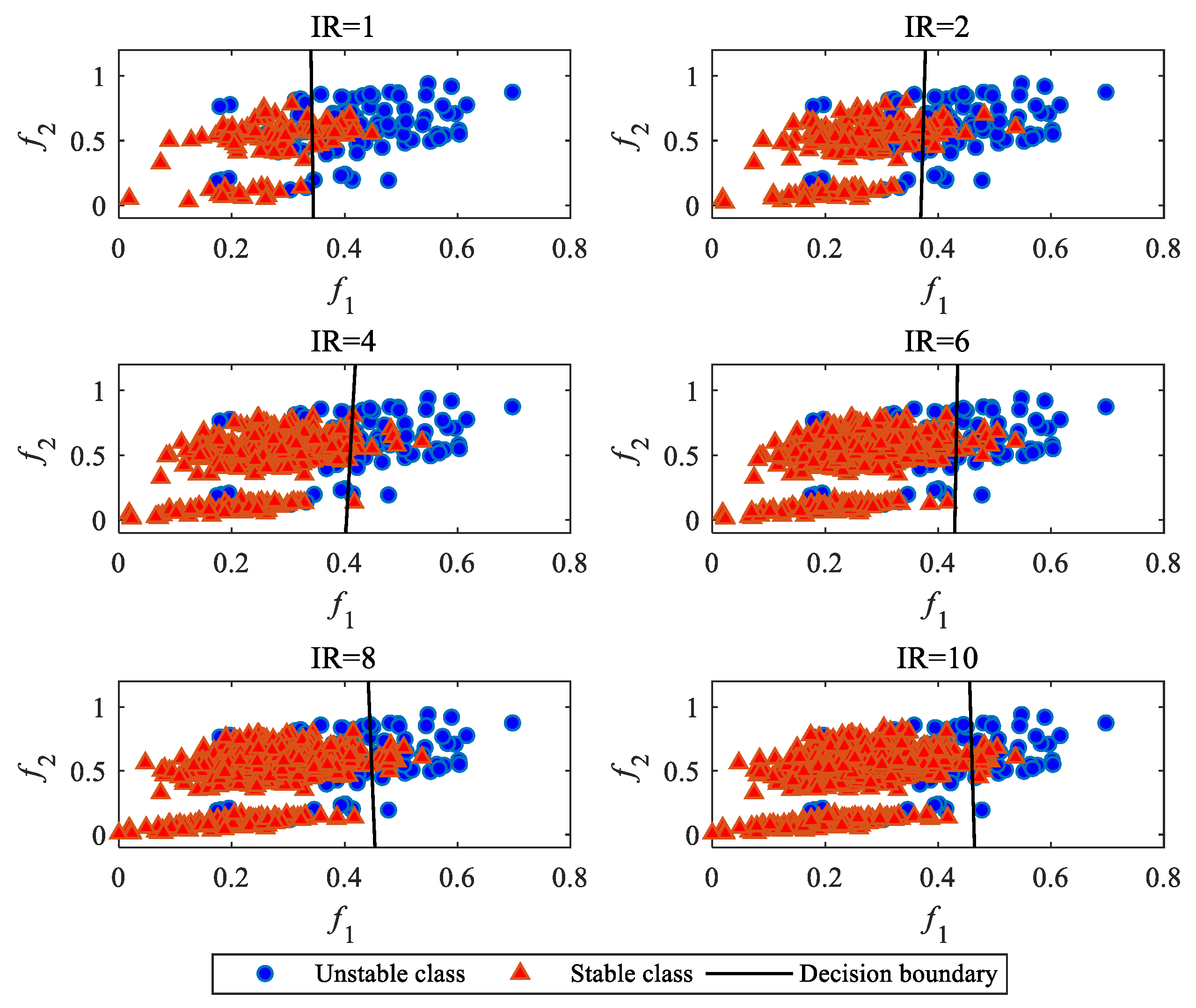
In order to illustrate the effect of IR on the decision boundary of the classification model, the IEEE 39-bus system is taken as the test system. Employing the approach proposed in our previous study [19], the database is generated and the importance of features is ranked. For visualization of the decision boundary, the top 2 features, f1 and f2, are utilized to build the classification model. Here, f1 represents the variance of generator rotor angles at the fault clearing time and f2 is the mean absolute of the generator angular velocities at the fault clearing time.
To construct different training sets based on different IRs, the number of unstable samples is fixed to 100 and the number of stable samples is respectively chosen as 100 (IR = 1), 200 (IR = 2), 400 (IR = 4), 600 (IR = 6), 800 (IR = 8), and 1000 (IR = 10). The logistic regression method is employed as the classifier. The decision boundaries of the classifier under different IRs are all depicted in Figure 2.
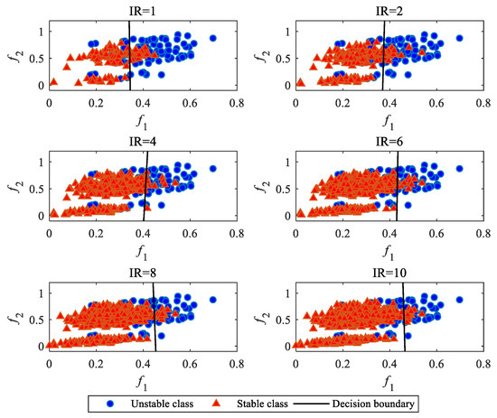
Figure 2.
Decision boundaries under different imbalanced ratios (IRs).
It can be seen from Figure 2 that as the IR increases, the decision boundary of classification model gradually shifts towards the unstable class that has fewer samples.
2.3. The Effect on the Classification Performance
Generally, the classification performance of TSSP can be characterized by the confusion matrix shown in Table 1.

Table 1.
Confusion matrix of TSSP.
The true stable class rate (TSR) and the true unstable class rate (TUR), utilized as the classification performance indexes of TSSP, are defined respectively as follows:
In addition to using the TSR and TUR as the performance indexes for stable class and unstable class, respectively, the geometric mean (GM) of TSR and TUR is also employed to measure the overall classification performance of TSSP [20] and the expression of GM is shown as follows:
The value of GM is not affected by the IR, so it is more suitable than the overall classification accuracy when dealing with the imbalanced data problem. The value of GM ranges from 0 to 1. The higher the value, the better the overall classification performance of TSSP.
The classification performance of TSSP is analyzed and compared under different IRs, shown in Table 2.

Table 2.
Confusion matrix of TSSP.
From Table 2, when IR = 1, the values of TSR and TUR are almost the same. With the increase of IR, the TSR gradually increases and then remains unchanged, while the TUR continues to decrease. When IR = 10, the TSR increases to 98.40% and the TUR decreases to 33.00%. In addition, as IR increases, the GM value first increases and then decreases. When IR = 2, the GM reaches its highest value, which is 78.66%. The results clearly validate that the imbalanced data problem dramatically deteriorates the classification accuracy of the unstable class, which seriously hinders the application of machine learning methods for TSSP.
3. The Proposed DSEC Method
From the analysis in Section 2, the imbalanced data problem in the training set deteriorates the classification performance of the TSSP model. To address this challenge, the DSEC method is proposed for TSSP. The detailed description of this method is shown in the following.
3.1. Data Segmentation Strategy
The training set in the TSSP problem can be divided into the stable set and the unstable set, and the stable samples usually outnumber the unstable samples. To obtain a relatively balanced training set, the data segmentation strategy is proposed. The basic idea of the data segmentation strategy is to divide the stable set into multiple non-overlapping stable subsets, ensuring that the samples in each stable subset are not more than the unstable samples.
The specific processes of data segmentation strategy are shown below.
Step 1: Given the stable set S with NS samples and the IR value, determine the number of stable subset T by
where ceil represents the ceiling function.
Calculate the remainder P by
Set k and P0 both equal to 1.
Step 2: If P0 ≤ P, go to step 3; otherwise go to step 4.
Step 3: Determine the number of samples in stable subset Sk by
Create the stable subset Sk by randomly selecting |Sk| samples from stable set S without replacement. Set P0 = P0 + 1, k = k + 1, then go to step 5.
Step 4: Determine the number of samples in stable subset Sk by
Create the stable subset Sk by randomly selecting |Sk| samples from stable set S without replacement. Set k = k + 1.
Step 5: If k ≤ T, return to step 2; otherwise go to step 6.
Step 6: Output T stable subsets S = {S1, S2, …, ST}.
From the strategy hereinbefore, if IR is an integer, the number of samples in each stable subset is the same as that of unstable samples. If not, the number of samples in each stable subset is less than that of unstable samples.
3.2. AdaBoost Algorithm
As a widely used machine learning method, AdaBoost is employed as the classifier in this paper. With the advantages of a sound theoretical foundation and simple implementation [21], it has been applied to many classification problems in practice [22,23].
Since AdaBoost itself is also an ensemble learning method, the classification and regression tree (CART) is adopted as its base learner and the basic processes of the AdaBoost algorithm are described as follows:
Step 1: Given the training set D = {(x1, y1), (x2, y2), …, (xN, yN)}, yi ∈ {−1, +1}, set the iteration round to R.
Step 2: Set r = 1, and initialize the weight of sample i, i = 1, …, N
Step 3: Create Dr by randomly selecting N samples from D with the probability ωr(i).
Step 4: Train the CART hr by using Dr.
Step 5: Calculate the classification error on D.
Step 6: Calculate the weight αr of CART hr.
Step 7: Update the weight distribution.
Set r = r + 1, if r ≤ R, return to step 3; otherwise go to step 8.
Step 8: Output decision value.
3.3. The DSEC Method
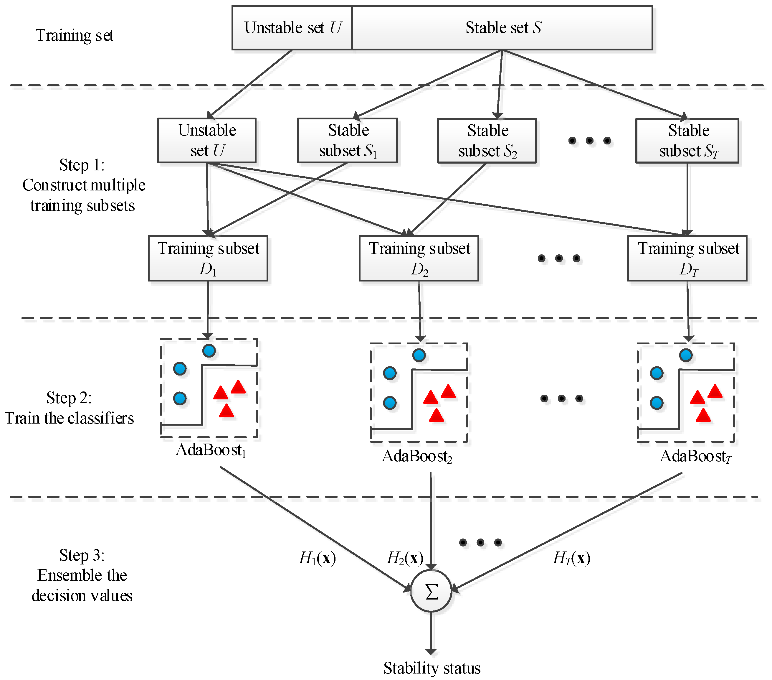
To solve the imbalanced data problem of TSSP, the three-step DSEC method is proposed. The descriptions of each step are summarized below.
Step 1: Divide the training set D into stable set S and unstable set U. Next, utilize the data segmentation strategy to split the stable set into T stable subsets, S = {S1, S2, …, ST}. Then, combine each stable subset with unstable set U into T training subsets, D = {D1, D2, …, DT}. If IR is an integer, the stable samples are as many as the unstable samples in each training subset; otherwise, the unstable samples are more than the stable samples in each training subset.
Step 2: Train T AdaBoost classifiers with T training subsets independently.
Step 3: Ensemble the decision values from T AdaBoost classifiers by using the summation rule expressed as follows:
Then, determine the transient stability status by
The schematic diagram of DSEC method is shown in Figure 3:
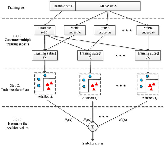
Figure 3.
Schematic diagram of the DSEC method.
4. The DSEC Method for TSSP
4.1. Database Generation and Preprocessing
In order to generate a statistical database for TSSP, the Monte Carlo method is utilized and the main steps of data generation and preprocessing are described as follows:
Step 1: Utilize the Monte Carlo method to randomly generate a new operating condition of the power system based on the base condition. Check the feasibility of the new operating condition and then randomly generate a disturbance scenario. Obtain the response trajectories of generators after given the disturbance scenario using the TDS method.
Step 2: Construct the initial features for the TSSP consisting of system-level features and single machine-level features. The electrical variables closely related to the transient stability characteristics, such as load level, generator active power output, rotor angle, kinetic energy, etc., are considered. A detailed feature description can be found in Reference [19].
Step 3: Determine the transient stability status of the power system. If the power system is unstable, it is labeled as 1; otherwise, it is stable, labeled as −1.
Step 4: Combine the initial features with the corresponding label to form a sample and put the sample into the database.
Step 5: Repeat steps 1–4 until the predefined number of samples is obtained.
Step 6: Employ the two-stage feature selection method [19] to eliminate the irrelevant and redundant features in the original database and, finally, obtain the classification database.
4.2. Flowchart of the DSEC Method for TSSP
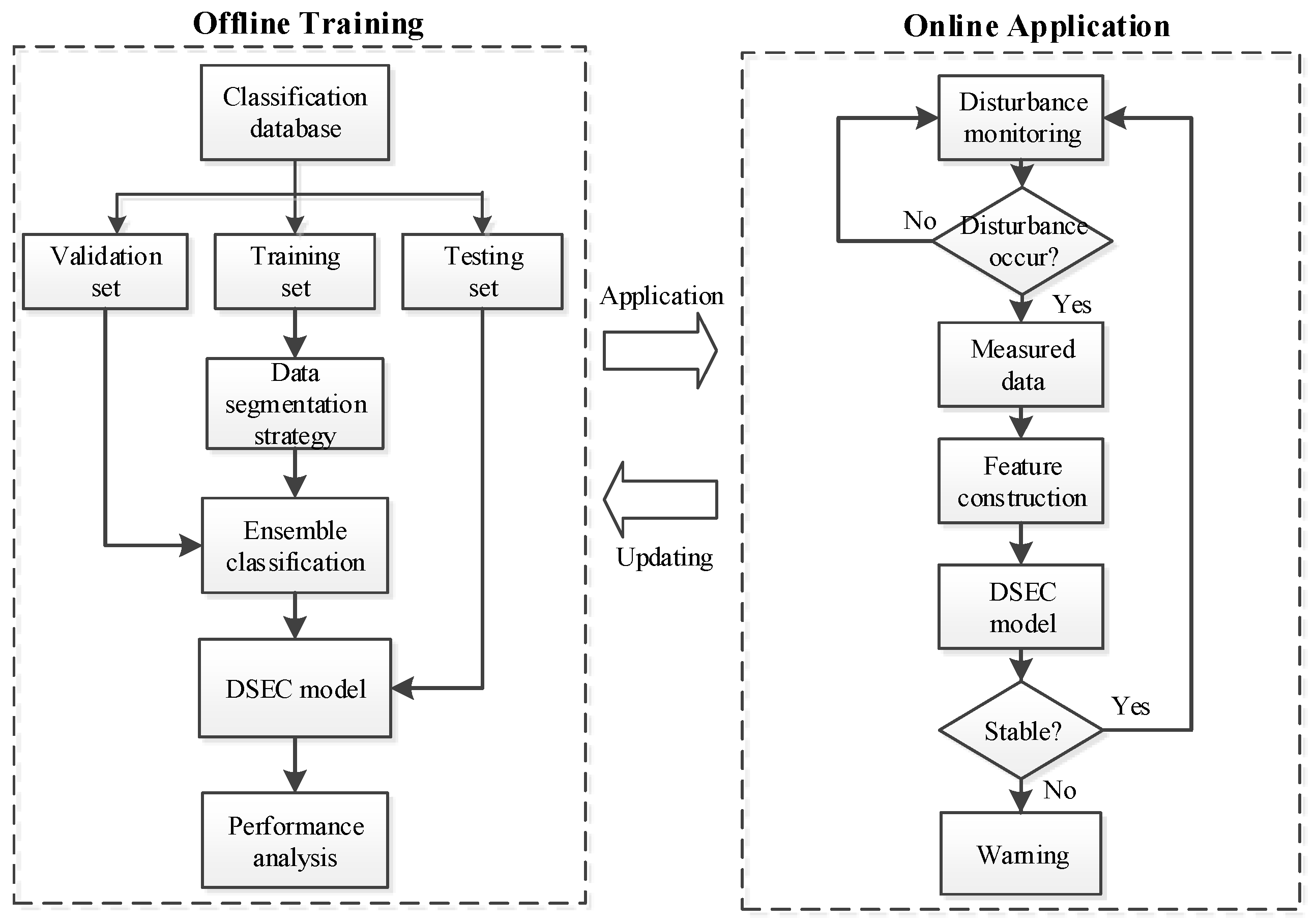
The proposed framework of the DSEC method for TSSP involves two stages: (1) Offline training and (2) online application, which are described respectively below:
- (1)
- Offline Training: The classification database is randomly divided into three parts, as follows: Training set, validation set, and testing set. The training set is split by the data segmentation strategy and then utilized for training multiply AdaBoost classifiers. The validation set is used for selecting the optimal parameter of the classifier and the testing set is utilized for evaluating the classification performance of the DSEC model for TSSP.
- (2)
- Online Application: The monitoring information of power systems is utilized to judge whether the system is subjected to a disturbance or not. If a disturbance occurs, the measured data is adopted to construct the input features and the stability status is predicted immediately after feeding these features into the DSEC model. If the system is predicted to have an unstable status, the system operator is immediately alerted to take proper control strategies to prevent large-scale outages. During online application, if significant changes happen to the operating condition or grid topology, the classification database should be updated immediately so that the DSEC model can be retrained for robustness improvement.
The flowchart of the proposed DSEC method for TSSP is shown in Figure 4:

Figure 4.
Flowchart of the DSEC method for TSSP.
5. Case Studies
The Northeast Power Coordinating Council (NPCC) 140-bus system, representing the equivalent power grid in the Northeastern United States, is utilized as a test system [24,25]. The simulations are carried out in MATLAB environment on a computer with an Intel Core i5 3.3 GHZ processor and 8 GB of RAM.
For database generation, the active power output and the terminal voltage of generators vary within ±20% and ±2% of the base operating condition, respectively, and the active and reactive power of loads both vary within ±20% of the base operating condition. A transmission line with permanent three-phase short-circuit is randomly selected as the fault condition and the fault duration is set to 0.12 s.
A total of 16,000 samples with 270 features are generated to form the original database of the TSSP. After two-stage feature selection preprocessing, 87 features are retained and the classification database is formed. A total of 60% of the classification database are randomly selected as the training set. Another 20% are randomly selected as the validation set and the remaining 20% are formed as the testing set. The sample distribution is shown in Table 3.

Table 3.
Sample distribution in the classification database.
From Table 3, there is an obvious imbalanced data problem in the classification database and the number of stable samples is about 4.8 times the number of unstable samples.
After applying the data segmentation strategy, the sample distribution in each training subset is tabulated in Table 4.

Table 4.
Sample distribution in each training subset.
5.1. Parameter Selection
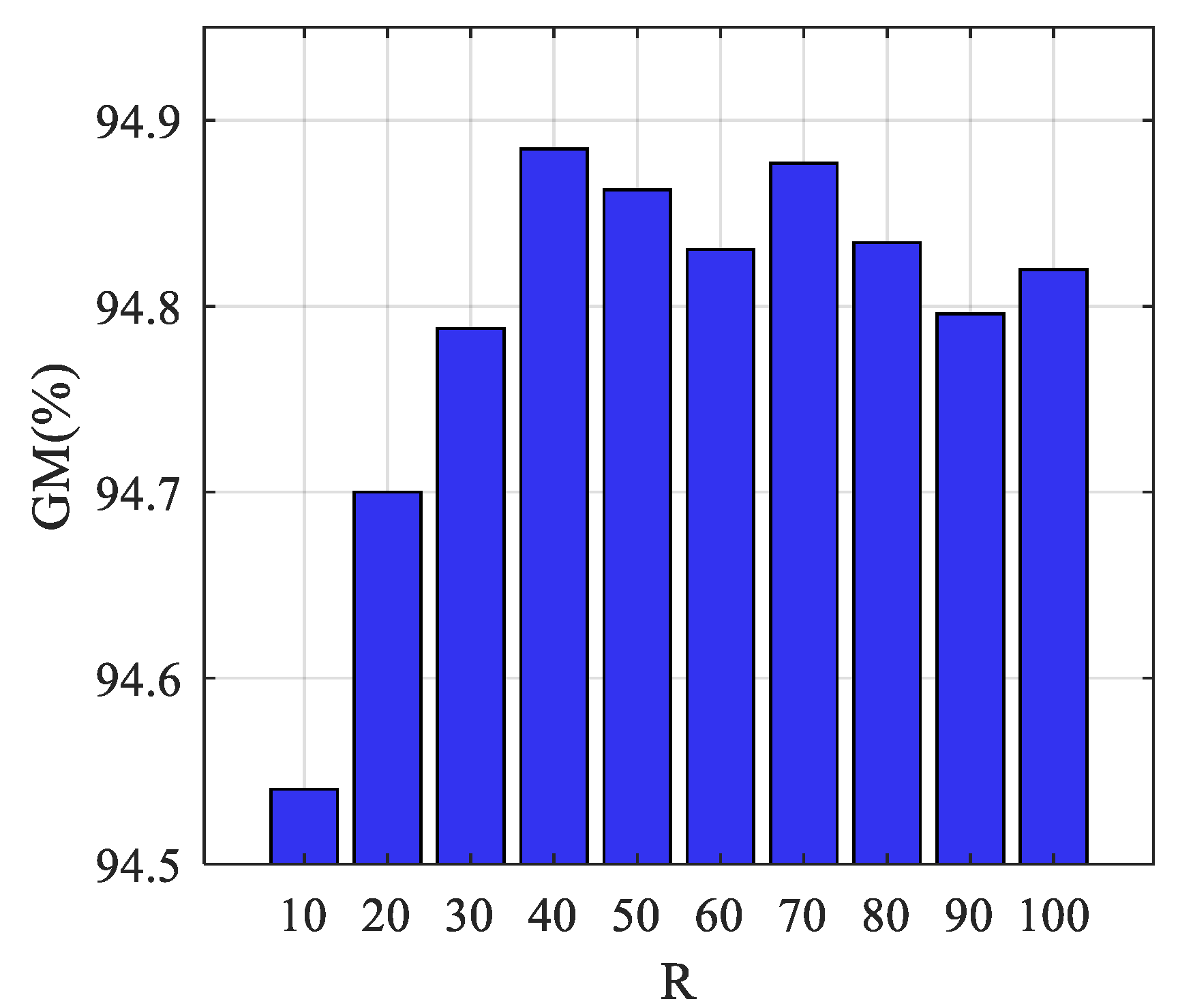
The main parameter of the DSEC model is iteration round R. Under different values of R, the GM performances of the DSEC model on the validation set are analyzed and compared and the value range is set to [10, 20, …, 100]. The results of parameter analysis are shown in Figure 5. Taking into account the randomness of the AdaBoost classifier, the average results of 10 repeated experiments are utilized for comparison.

Figure 5.
GM performance with different values of R.
It can be seen from Figure 5 that, with the increase of R, the GM value increases rapidly at first and then gradually remains stable. Considering the classification performance and model complexity, the value of R is set to 40.
5.2. Comparison with Traditional Machine Learning Methods
In this section, a comparison is made between the DSEC model and the traditional machine learning methods including SVM, ELM, CART, and AdaBoost, which do not consider the imbalanced data problem. The Gaussian function is chosen as the kernel function of SVM, and its parameters includes the penalty coefficient, c, and the kernel function parameter, γ. The grid search method is utilized for selecting the optimal parameters of SVM and the value range of both parameters is [2–8, 2–7, …, 28]. The main parameter of ELM is the number of hidden layer nodes, L, and its range is set as [50, 100, ..., 1500]. The default parameters are adopted in the CART algorithm and the iteration round of the AdaBoost classifier is 40.
The results of these methods for TSSP are compared and tabulated in Table 5.

Table 5.
Results comparison with traditional machine learning methods.
From Table 5, when dealing with the TSSP problem with imbalanced data, the traditional machine learning methods lead to a high TSR but quite low TUR and GM. While the proposed DSEC model can significantly improve the TUR and GM, which become as high as 97.03% and 94.62% respectively, with the TSR still being maintained at 92.28%.
5.3. Comparison with Other Data-Level Methods
In this section, the DSEC method is compared with some state-of-the-art data-level methods for imbalanced TSSP problem, including random oversampling (ROS) [14], random undersampling (RUS) [20], the synthetic minority over-sampling technique (SMOTE) [26], ADASYN, cluster-based undersampling (CUS) [27], and EasyEnsemble [20]. The detailed processes using these methods for the imbalanced data problem of TSSP are described as follows:
- (1)
- ROS: A new unstable set UROS is sampled with replacement from the original unstable set U, so that |UROS| = NS. Then the unstable set UROS is combined with stable set S to form a new training set.
- (2)
- RUS: A new stable set, SRUS, is sampled with replacement from the original stable set, S, so that |SROS| = NU. Then the stable set SRUS is combined with stable set U to form a new training set.
- (3)
- SMOTE: New NS-NU unstable samples are generated by using SMOTE. Then, these unstable samples are added into the original training set, so that |USMOTE | = NS in the new training set.
- (4)
- ADASYN: New NS-NU unstable samples are generated by using ADASYN. Then, these unstable samples are added into the original training set, so that |UADASYN| = NS in the new training set.
- (5)
- CUS: The k-mediods algorithm is used for clustering the stable samples with NU clusters. A new unstable set UCUS is constructed with the NU samples from cluster center, so that |UCUS| = NS. Then the unstable set UCUS is combined with stable set S to form a new training set.
- (6)
- EasyEnsemble: Randomly sample a stable subset SEasy from the original stable set S, so that |SEasy| = NU. Then the stable set SEasy is combined with stable set U to form a new training subset. Repeat above process TEasy times and obtain TEasy training subsets. Here, TEasy is set to 5.
The AdaBoost classifier is employed for data-level methods hereinbefore, and considering the randomness of these methods, the average results of 10 repeated experiments are taken for comparison. The training time and classification results of these methods are compared and shown in Table 6.

Table 6.
Results comparison of imbalanced data process methods.
From Table 6, the DSEC method has higher TUR and GM values than other imbalanced data process methods, which means that the proposed method has a better classification performance both in unstable samples and overall samples and costs relatively less training time than other methods, except RUS. Therefore, the DSEC method is superior for TSSP with imbalanced data. Furthermore, the total time cost of DSEC method on testing data is 0.20 s, i.e., the computation time of one sample, is about 0.06 ms, which demonstrates the feasibility of applying the method for online application.
5.4. The Performance of the DSEC Method Under Different IRs
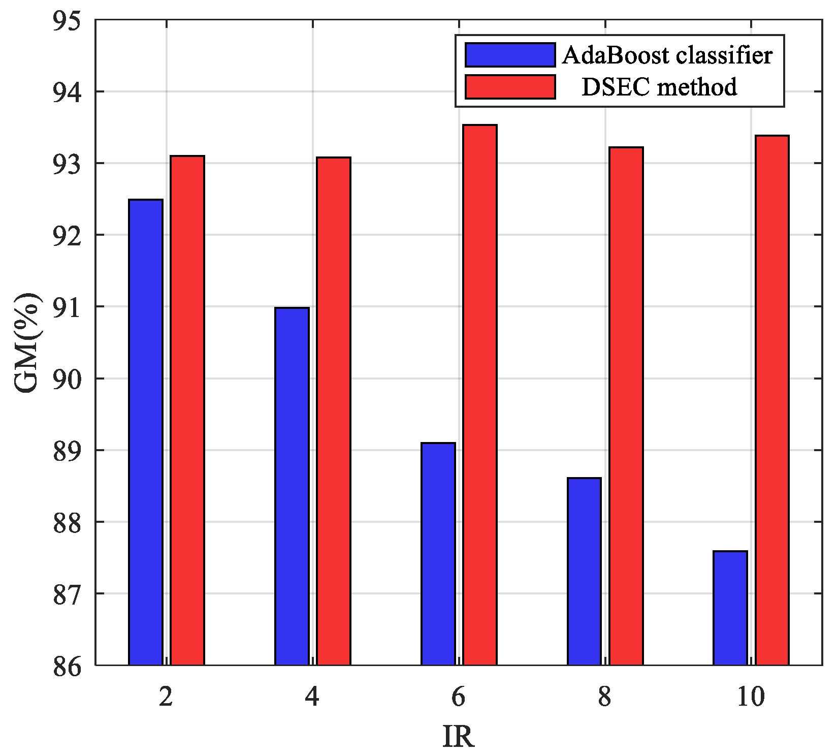
In order to study the classification performance of the DSEC method under different IRs, the value range of IR is set to [2, 4, ..., 10] and new training sets and testing sets for studying are constructed based on the value of IR. The GM performance of the DSEC method is evaluated under different IRs. In addition, as a traditional machine learning method, the AdaBoost classifier is utilized for comparing with the DSEC method using the same sample set. The results of these two methods are illustrated and compared in Figure 6.

Figure 6.
GM performance comparison under different IRs.
As the IR increases, the GM performance of the AdaBoost classifier decreases continuously and when IR = 10, the GM value decreases to about 87%. The performance of the DSEC method is almost unaffected with the change of IR and all the GM values are all higher than 93% under different IRs. The results further demonstrate the effectiveness of the DSEC method in dealing with the imbalanced data problem of TSSP.
Under different IRs, the increment of GM (IGM) value of the DSEC method over the AdaBoost classifier is shown in Table 7.

Table 7.
IGM values under different IRs.
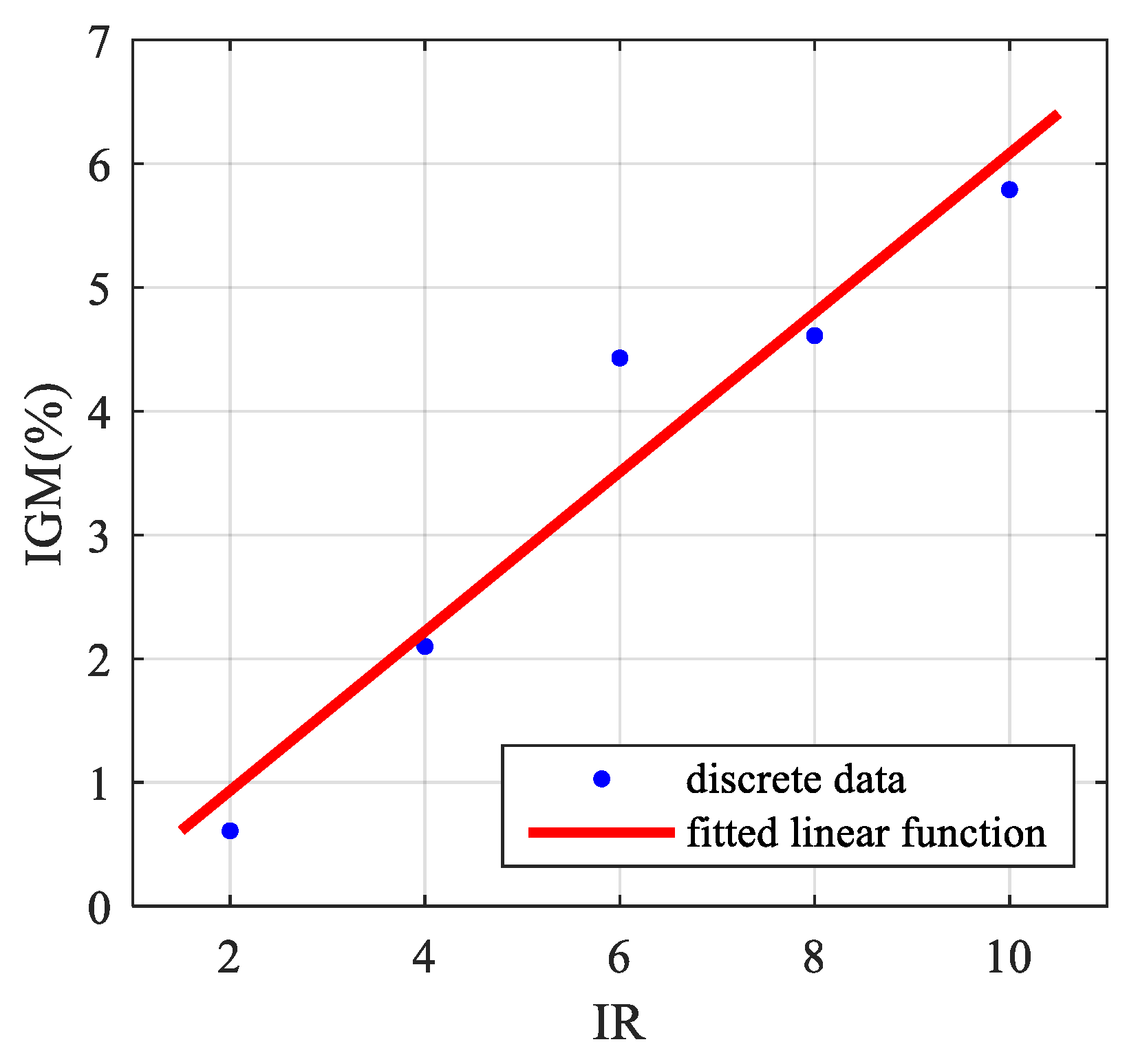
An approximate linear function between the IR and the IGM value is fitted as follows:
The discrete data points and the fitted linear function are shown in Figure 7.
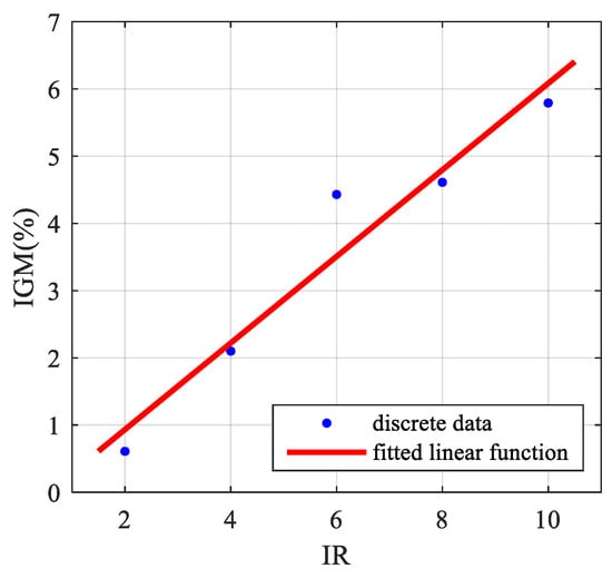
Figure 7.
Relationship between IR and IGM.
As shown in Figure 7, the IGM value almost increases linearly with the increase of IR, which means that the more severe the imbalanced data problem of TSSP, the greater the improvement of the DSEC method over the AdaBoost classifier makes.
6. Conclusions
This paper proposes the DSEC method to deal with the imbalanced data problem of TSSP. Firstly, the effects of the imbalanced data problem on the decision boundary and the classification performance of TSSP are analyzed in detail. Then, the three-step DSEC method is proposed to handle this problem. Finally, the effectiveness is demonstrated on the NPCC 140-bus system. The conclusions are drawn as follows:
- (1)
- The imbalanced data problem can seriously deteriorate the classification performance of TSSP.
- (2)
- Compared with traditional machine learning methods, the proposed DSEC method can significantly improve the TUR and GM of TSSP, with the TSR value still being kept at a high level.
- (3)
- Compared with state-of-the-art data-level methods, the proposed DSEC method has higher TUR and GM values. Furthermore, the rapidity of the DSEC method fully meets the requirement of online application of TSSP.
- (4)
- The proposed DSEC method maintains a high GM value under different IRs. Moreover, the higher the IR value is, the greater the advantage of DSEC method over traditional machine learning methods will have.
Author Contributions
Z.C. and X.H. developed the idea of this research and performed simulation verification; C.F. collected and processed the data; Z.C. and Z.H. wrote this paper; X.S. and S.M. checked and polished this paper.
Funding
This work was supported by Science and Technology Project of State Grid Sichuan Electric Power Company (No. 52199718001V).
Acknowledgments
The authors would like to appreciate Yuqin Chen from South Western University of Finance and Economics for her efforts in checking and polishing this paper. Also we would like to thank Pengfei Chen from Xihua University for his help in this paper.
Conflicts of Interest
The authors declare no conflict of interest.
References
- Kundur, P.; Paserba, J.; Ajjarapu, V.; Andersson, G.; Bose, A.; Canizares, C.; Hatziargyriou, N.; Hill, D.; Stankovic, A.; Taylor, C.; et al. Definition and classification of power system stability IEEE/CIGRE joint task force on stability terms and definitions. IEEE Trans. Power Syst. 2004, 19, 1387–1401. [Google Scholar]
- Zhou, Y.Z.; Guo, Q.L.; Sun, H.B.; Yu, Z.H.; Wu, J.Y.; Hao, L.L. A novel data-driven approach for transient stability prediction of power systems considering the operational variability. Int. J. Electr. Power 2019, 107, 379–394. [Google Scholar] [CrossRef]
- Meng, K.; Dong, Z.Y.; Wong, K.P.; Xu, Y.; Luo, F.J. Speed-up the computing efficiency of power system simulator for engineering-based power system transient stability simulations. IET Gener. Transm. Distrib. 2010, 4, 652–661. [Google Scholar] [CrossRef]
- Bhui, P.; Senroy, N. Real-time prediction and control of transient stability using transient energy function. IEEE Trans. Power Syst. 2017, 32, 923–934. [Google Scholar] [CrossRef]
- De La Ree, J.; Centeno, V.; Thorp, J.S.; Phadke, A.G. Synchronized phasor measurement applications in power systems. IEEE Trans. Smart Grid 2010, 1, 20–27. [Google Scholar] [CrossRef]
- Zhang, Y.C.; Xu, Y.; Dong, Z.Y.; Xu, Z.; Wong, K.P. Intelligent early warning of power Ssystem dynamic insecurity risk: Toward optimal accuracy-earliness tradeoff. IEEE Trans Ind. Inform. 2017, 13, 2544–2554. [Google Scholar] [CrossRef]
- Xu, Y.; Dong, Z.Y.; Meng, K.; Zhang, R.; Wong, K.P. Real-time transient stability assessment model using extreme learning machine. IET Gener. Transm. Distrib. 2011, 5, 314–322. [Google Scholar] [CrossRef]
- Yu, J.J.Q.; Hill, D.J.; Lam, A.Y.S.; Gu, J.T.; Li, V.O.K. Intelligent time-adaptive transient stability assessment system. IEEE Trans. Power Syst. 2018, 33, 1049–1058. [Google Scholar] [CrossRef]
- Gomez, F.R.; Rajapakse, A.D.; Annakkage, U.D.; Fernando, I.T. Support vector machine-based algorithm for post-fault transient stability status prediction using synchronized measurements. IEEE Trans. Power Syst. 2011, 26, 1474–1483. [Google Scholar] [CrossRef]
- Zhou, Y.Z.; Wu, J.Y.; Yu, Z.H.; Ji, L.Y.; Hao, L.L. A hierarchical method for transient stability prediction of power systems using the confidence of a SVM-based ensemble classifier. Energies 2016, 9, 778. [Google Scholar] [CrossRef]
- Amraee, T.; Ranjbar, S. Transient instability prediction using decision tree technique. IEEE Trans. Power Syst. 2013, 28, 3028–3037. [Google Scholar] [CrossRef]
- Liu, C.X.; Tang, F.; Leth Bak, C. An Accurate online dynamic security assessment scheme based on random forest. Energies 2018, 11, 1914. [Google Scholar] [CrossRef]
- Thirugnanasambandam, V.; Jain, T. AdaBoost classifiers for phasor measurements-based security assessment of power systems. IET Gener. Transmiss. Distrib. 2018, 12, 1747–1755. [Google Scholar] [CrossRef]
- Kamwa, I.; Samantaray, S.R.; Joos, G. catastrophe predictors from ensemble decision-tree learning of wide-area severity indices. IEEE Trans. Smart Grid 2010, 1, 144–158. [Google Scholar] [CrossRef]
- Tan, B.D.; Yang, J.; Tang, Y.F.; Jiang, S.B.; Xie, P.Y.; Yuan, W. A deep imbalanced learning framework for transient stability assessment of power system. IEEE Access 2019, 7, 81759–81769. [Google Scholar] [CrossRef]
- He, H.B.; Garcia, E.A. Learning from imbalanced data. IEEE Trans. Knowl. Data Eng. 2009, 21, 1263–1284. [Google Scholar]
- Chen, Z.; Xiao, X.Y.; Li, C.S.; Zhang, Y.; Hu, Q.Q. Real-time transient stability status prediction using cost-sensitive extreme learning machine. Neural Comput. Appl. 2016, 27, 321–331. [Google Scholar] [CrossRef]
- Zhu, L.P.; Lu, C.; Dong, Z.Y.; Hong, C. Imbalance learning machine-based power system short-term voltage stability assessment. IEEE Trans Ind. Inform. 2017, 13, 2533–2543. [Google Scholar] [CrossRef]
- Chen, Z.; Han, X.Y.; Fan, C.W.; Zheng, T.W.; Mei, S.W. A two-stage feature selection method for power system transient stability status prediction. Energies 2019, 12, 689. [Google Scholar] [CrossRef]
- Liu, X.Y.; Wu, J.X.; Zhou, Z.H. Exploratory undersampling for class-imbalance learning. IEEE Trans. Syst. Man Cybern. B Cybern. 2009, 39, 539–550. [Google Scholar]
- Freund, Y.; Schapire, R.E. A decision-theoretic generalization of on-line learning and an application to boosting. J. Comput. Syst. Sci. 1997, 55, 119–139. [Google Scholar] [CrossRef]
- Gamal, H.; Ismail, N.E.; Rizk, M.R.M.; Khedr, M.E.; Aly, M.H. A Coherent Performance for Noncoherent Wireless Systems Using AdaBoost Technique. Appl. Sci. 2019, 9, 256. [Google Scholar] [CrossRef]
- Wang, Y.B.; Ai, H.Z.; Wu, B.; Huang, C. Real time facial expression recognition with AdaBoost. In Proceedings of the 17th International Conference on Pattern Recognition, Cambridge, UK, 26 August 2004. [Google Scholar]
- Chow, J.H.; Cheung, K.W. A toolbox for power system dynamics and control engineering education and research. IEEE Trans. Power Syst. 1992, 7, 1559–1564. [Google Scholar] [CrossRef]
- Ju, W.Y.; Qi, J.J.; Sun, K. Simulation and analysis of cascading failures on an NPCC power system test bed. In Proceedings of the 2015 IEEE Power & Energy Society General Meeting, Denver, CO, USA, 26–30 July 2015. [Google Scholar]
- Chawla, N.V.; Bowyer, K.W.; Hall, L.O.; Kegelmeyer, W.P. SMOTE: Synthetic minority over-sampling technique. J. Artif. Intell. Res. 2002, 16, 321–357. [Google Scholar] [CrossRef]
- Lin, W.C.; Tsai, C.F.; Hu, Y.H.; Jhang, J.S. Clustering-based undersampling in class-imbalanced data. Inf. Sci. 2017, 409, 17–26. [Google Scholar] [CrossRef]
© 2019 by the authors. Licensee MDPI, Basel, Switzerland. This article is an open access article distributed under the terms and conditions of the Creative Commons Attribution (CC BY) license (http://creativecommons.org/licenses/by/4.0/).

