Estimating Road Segments Using Natural Point Correspondences of GPS Trajectories

Abstract
:1. Introduction
Task
2. Related Work
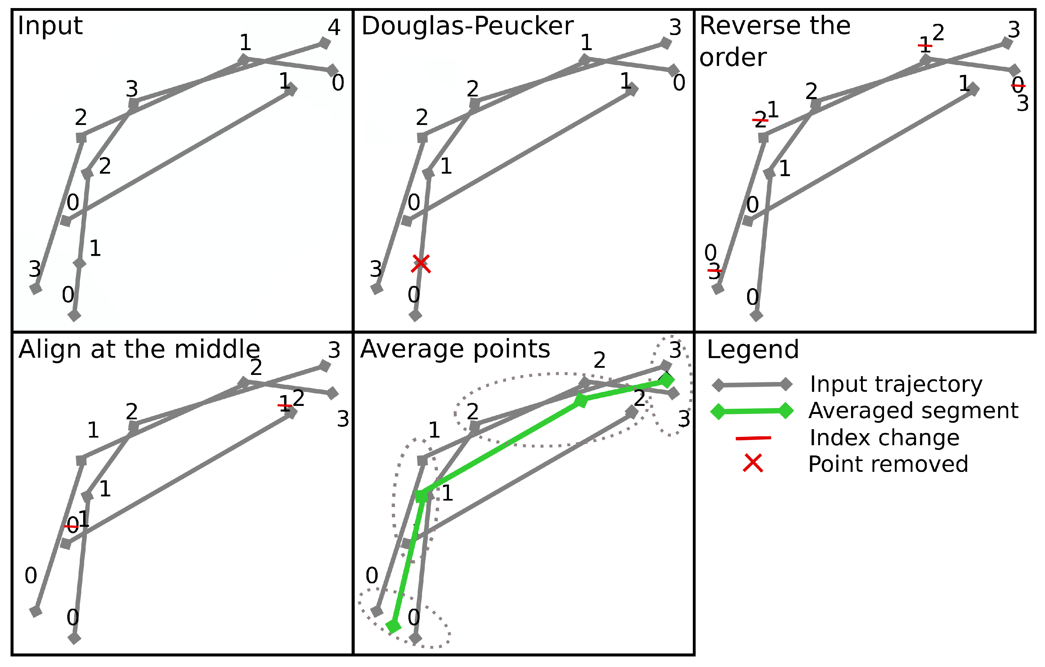
3. Method
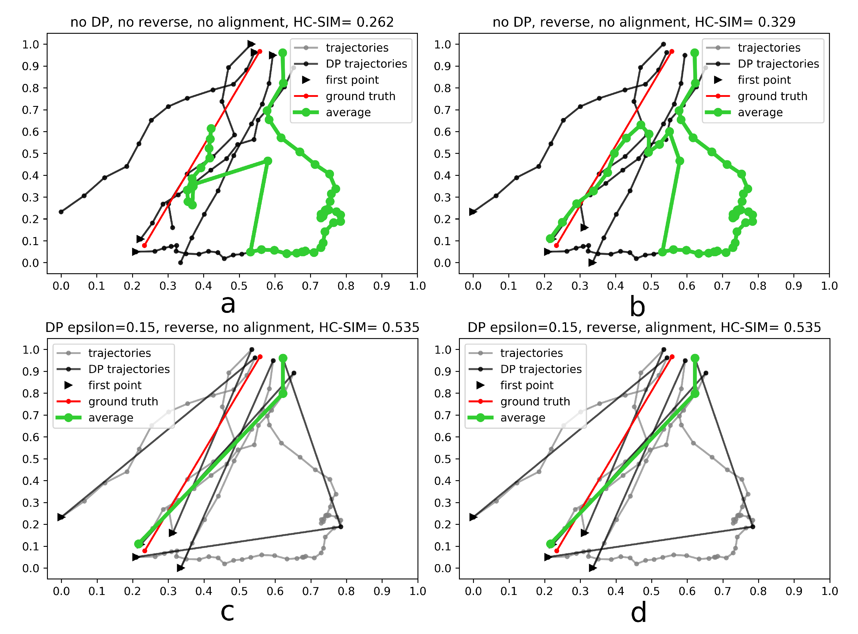
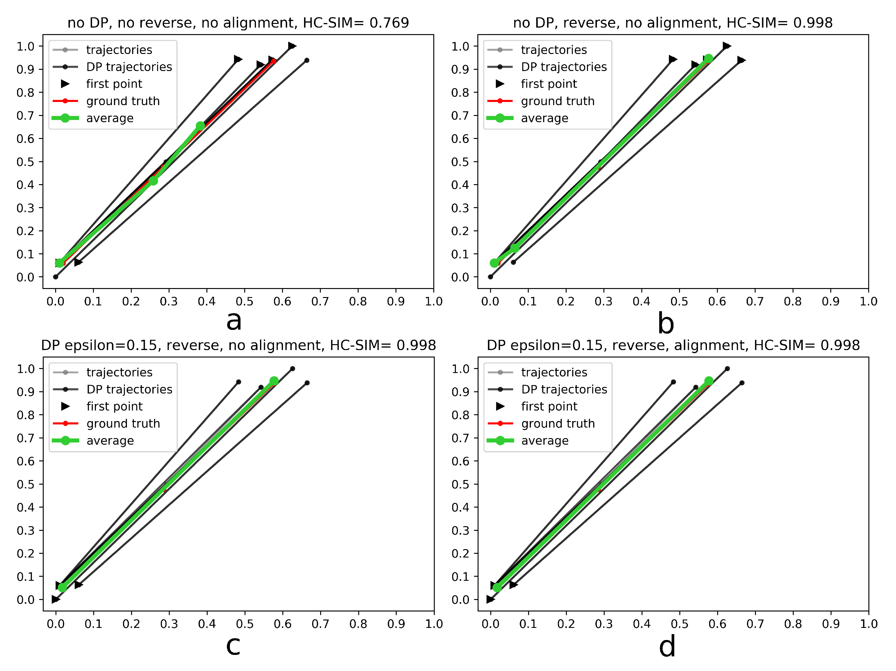
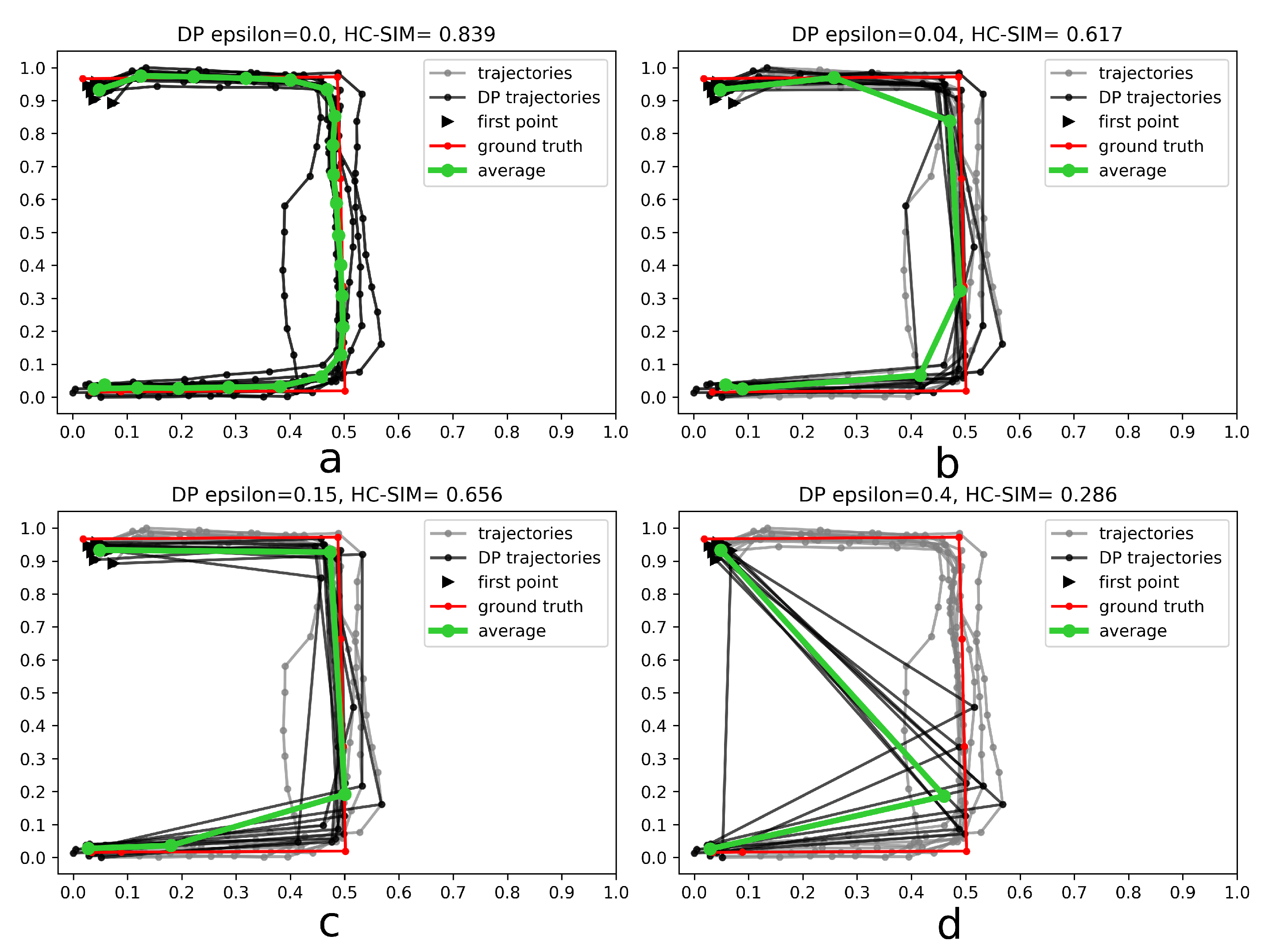
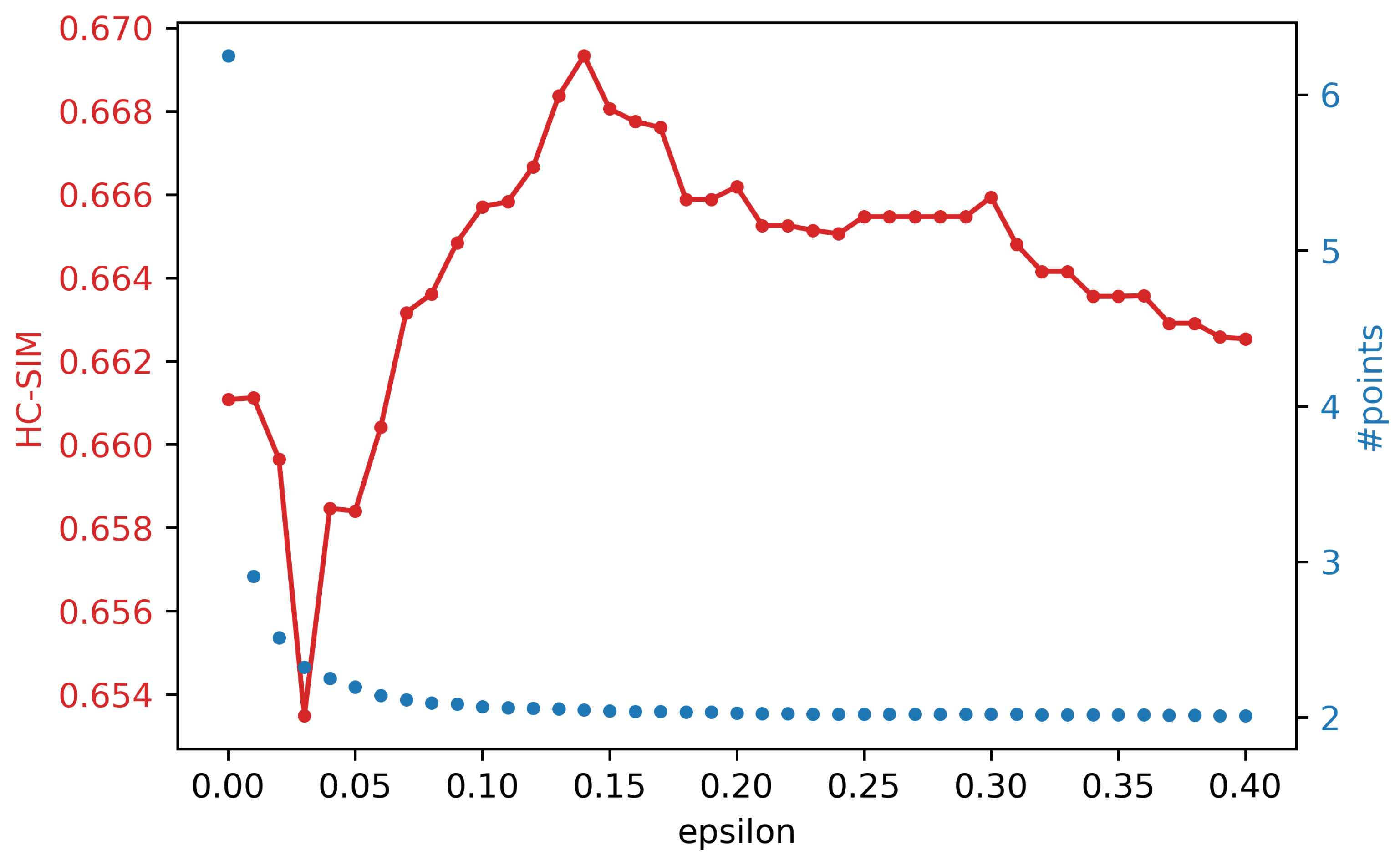
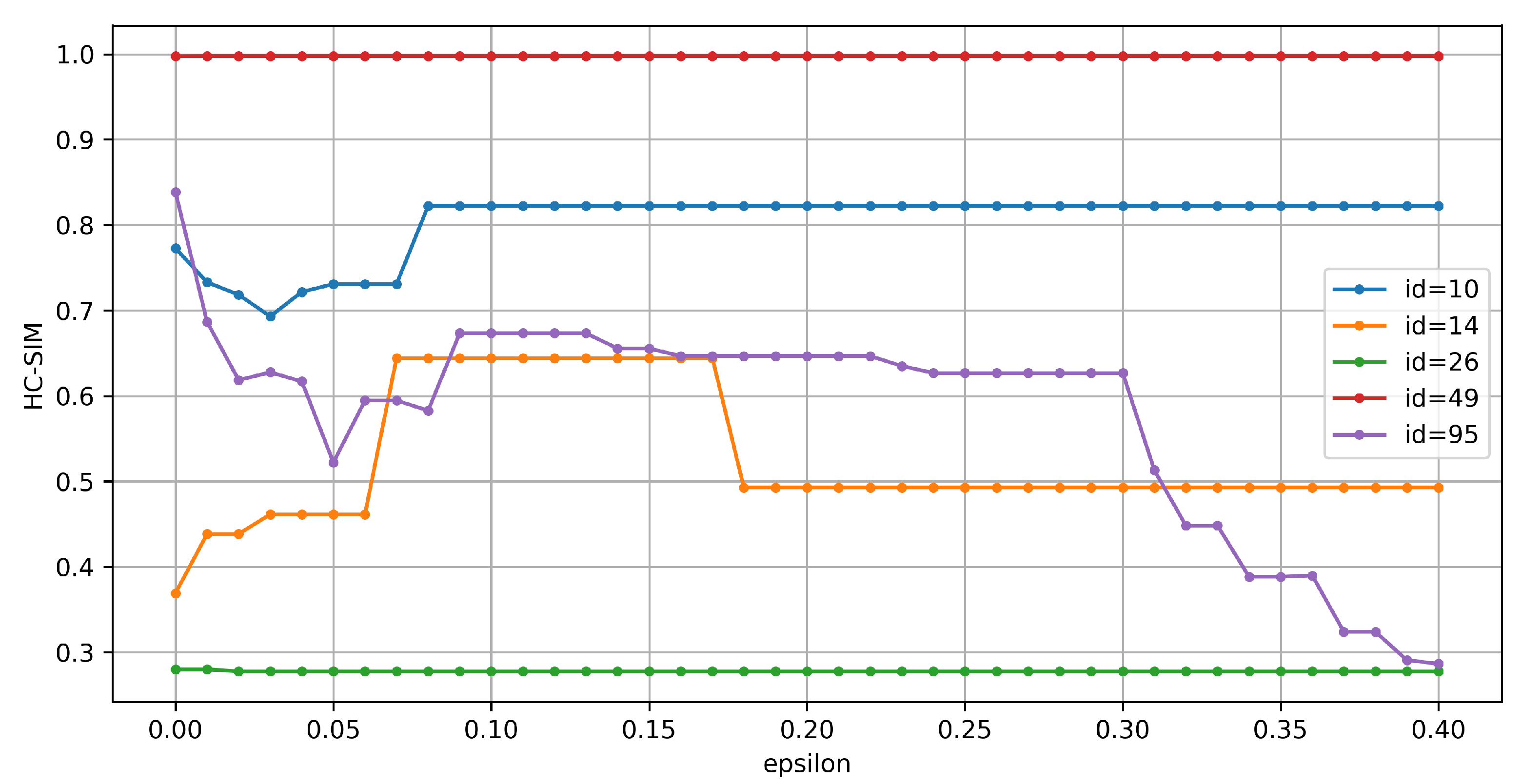
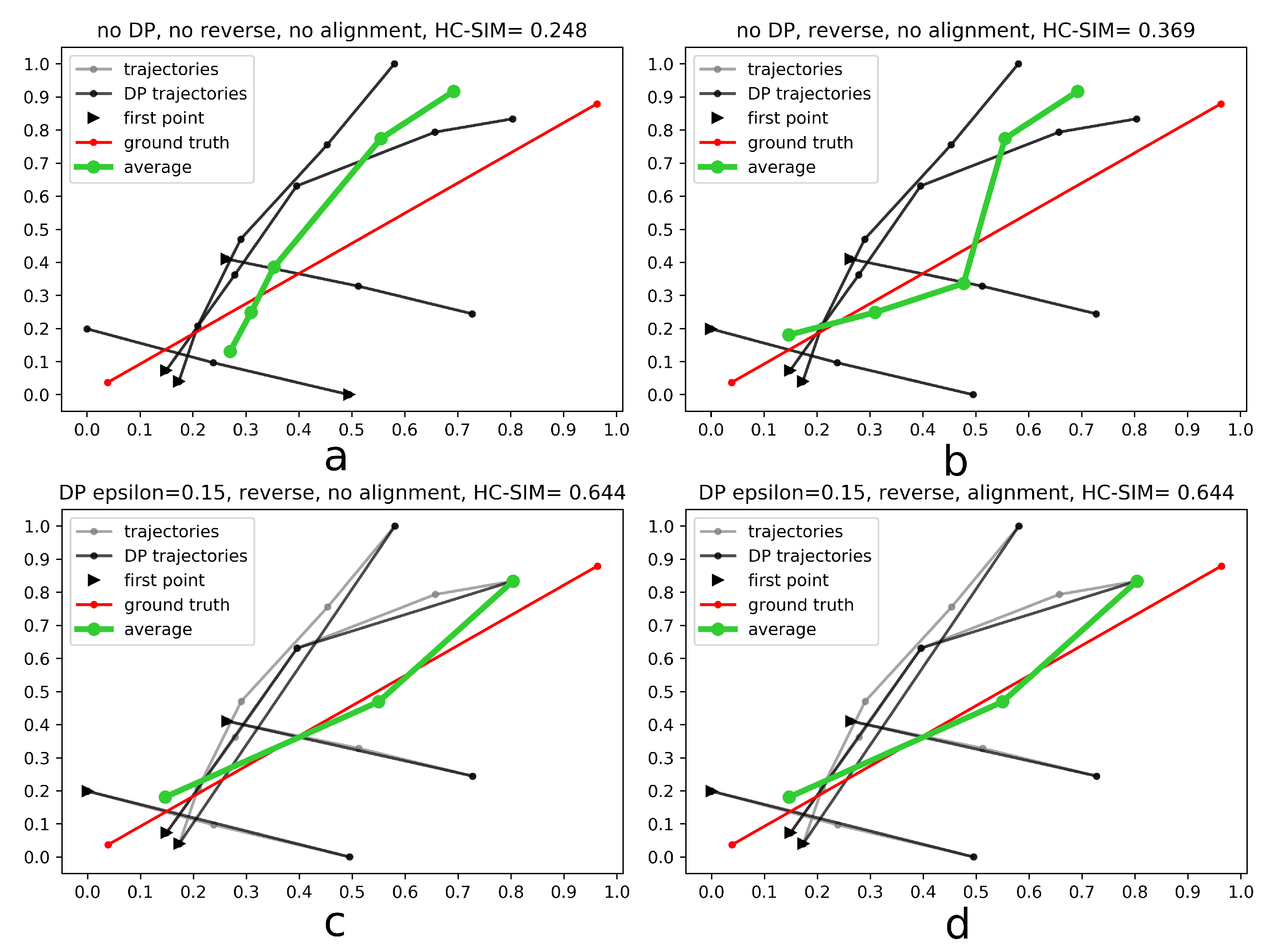
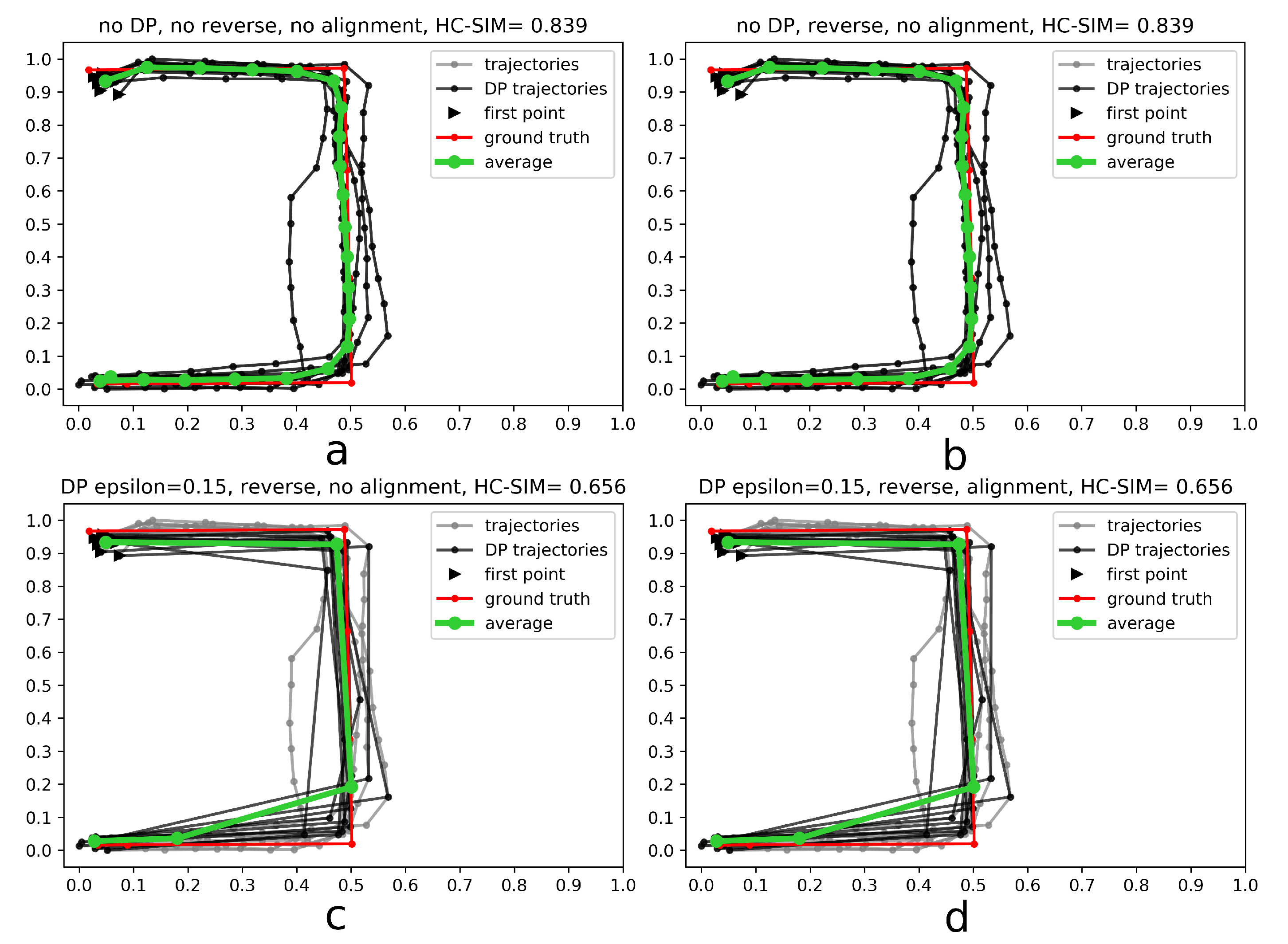
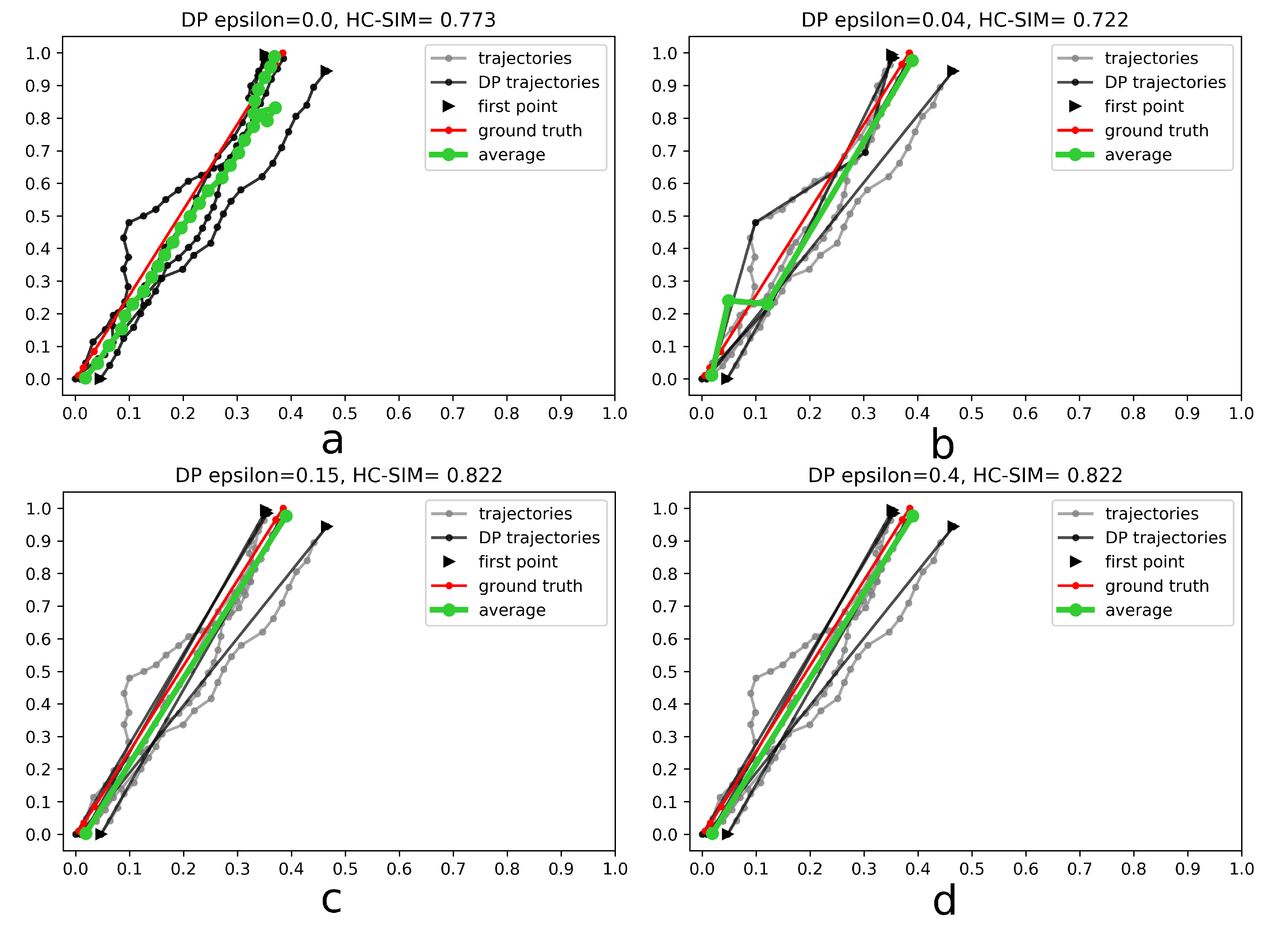
- Generalize single trajectories using the DP algorithm. DP takes a curve composed of segments defined by 2D points and creates a sketch by repeatedly adding the point with maximal orthogonal error to the sketch unless this error falls below a fixed threshold .
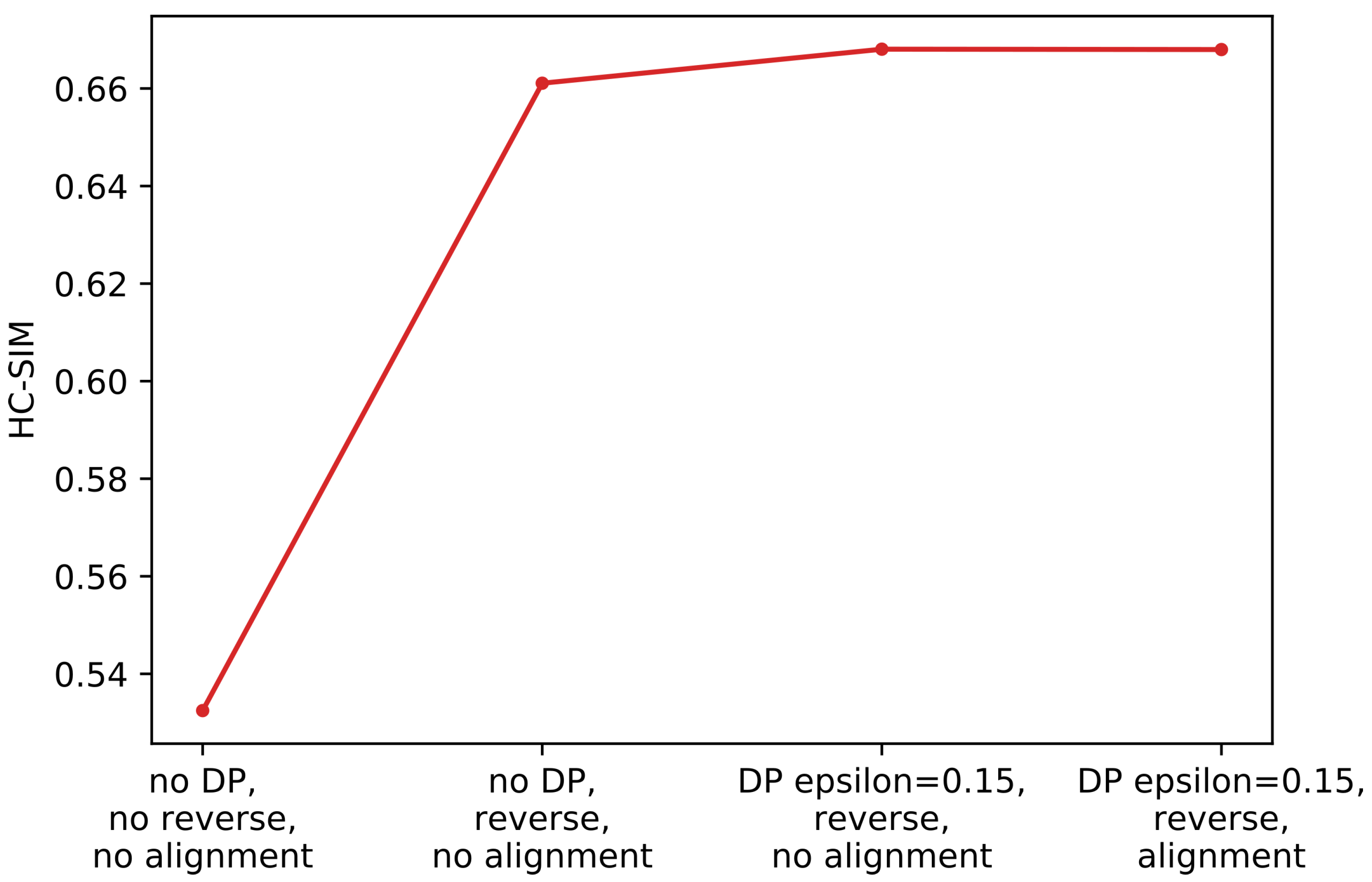
- Determine the trajectory that contains the most points. Reverse the order of the points in some trajectories to achieve identical orientation. The order of indices in a trajectory is reversed if the distance between the endpoint of and start point of is smaller than the distance between the start point of and the start point of .
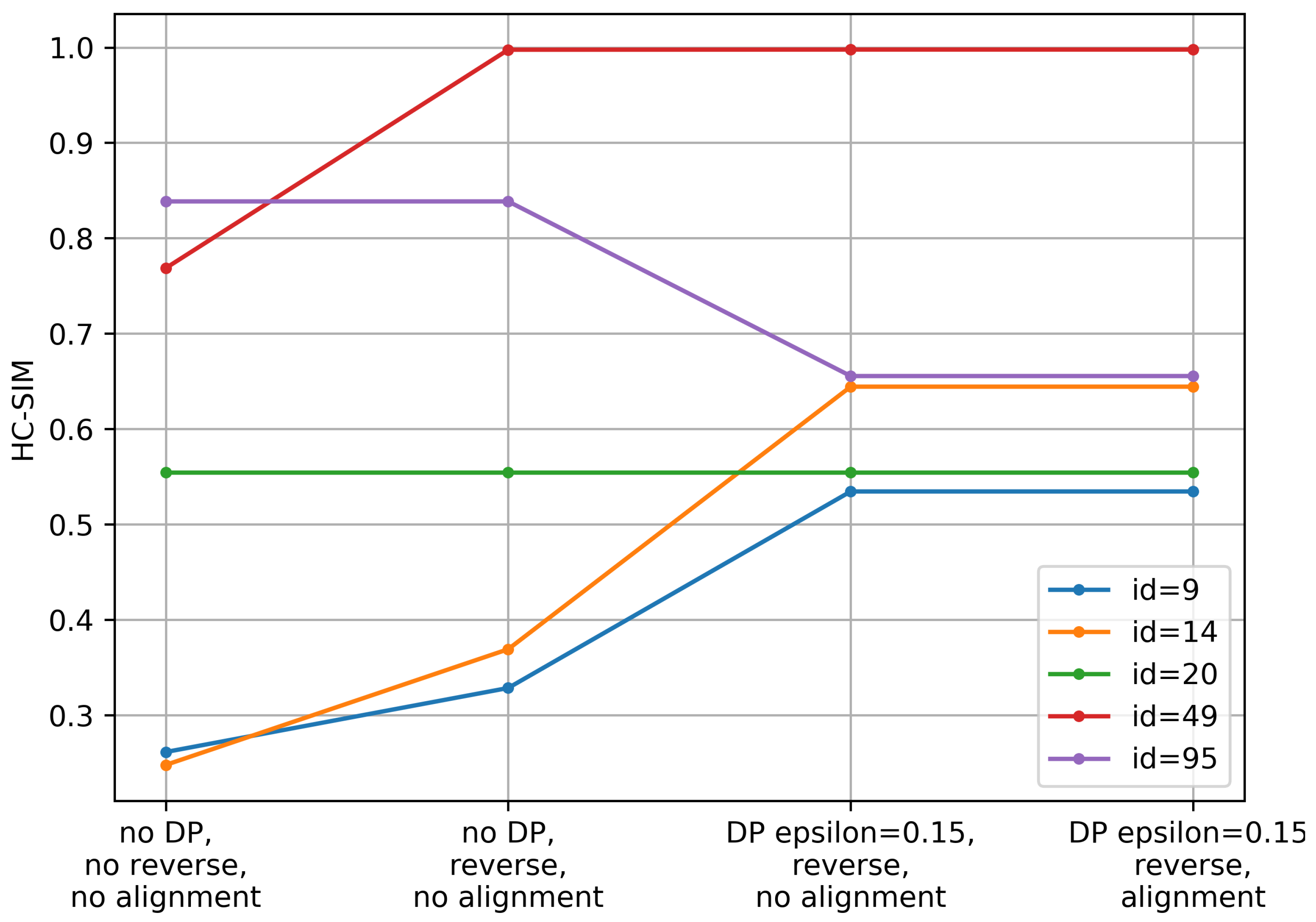
- Align indices of the points in trajectories with a smaller number of points along using linear interpolation. This step was part of the contribution to the contest, but as described in the Experiments and Discussion part this step is not always contributing to the performance improvement.
- Calculate the centroid of all points with the same index by averaging coordinates.
4. Experiments
4.1. Results
4.2. Competition Results and Relative Performance
4.3. Discussion
5. Conclusions
Author Contributions
Funding
Conflicts of Interest
Appendix A


References
- Zhang, Y.; Xiong, Z.; Zang, Y.; Wang, C.; Li, J.; Li, X. Topology-aware road network extraction via Multi-supervised Generative Adversarial Networks. Remote Sens. 2019, 11, 1017. [Google Scholar] [CrossRef]
- Li, P.; Zang, Y.; Wang, C.; Li, J.; Cheng, M.; Luo, L.; Yu, Y. Road network extraction via deep learning and line integral convolution. In Proceedings of the 2016 IEEE International Geoscience and Remote Sensing Symposium (IGARSS), Beijing, China, 10–15 July 2016; pp. 1599–1602. [Google Scholar] [CrossRef]
- Koetsier, C.; Busch, S.; Sester, M. Trajectory extraction for analysis of unsafe driving behaviour. ISPRS Int. Arch. Photogramm. Remote Sens. Spatial Inf. Sci. 2019, XLII-2/W13, 1573–1578. [Google Scholar] [CrossRef]
- Zourlidou, S.; Sester, M. Intersection detection based on qualitative spatial reasoning on stopping point clusters. ISPRS Int. Arch. Photogramm. Remote Sens. Spatial Inf. Sci. 2016, XLI-B2, 269–276. [Google Scholar] [CrossRef]
- Seidl, D.E.; Jankowski, P.; Tsou, M.H. Privacy and spatial pattern preservation in masked GPS trajectory data. Int. J. Geogr. Inf. Sci. 2016, 30, 785–800. [Google Scholar] [CrossRef]
- Fränti, P.; Mariescu-Istodor, R. Averaging GPS segments challenge 2019. Unpublished work. 2019. [Google Scholar]
- Mariescu-Istodor, R.; Fränti, P. CellNet: Inferring Road Networks from GPS Trajectories. ACM Trans. Spat. Algorithms Syst. 2018, 4, 8:1–8:22. [Google Scholar] [CrossRef]
- Ni, Z.; Xie, L.; Xie, T.; Shi, B.; Zheng, Y. Incremental road network generation based on vehicle trajectories. ISPRS Int. J. Geo-Inf. 2018, 7, 382. [Google Scholar] [CrossRef]
- Li, D.; Li, J.; Li, J. Road Network Extraction from Low-Frequency Trajectories Based on a Road Structure-Aware Filter. ISPRS Int. J. Geo-Inf. 2019, 8, 374. [Google Scholar] [CrossRef]
- Fathi, A.; Krumm, J. Detecting road intersections from GPS traces. In Proceedings of the International Conference on Geographic Information Science, Zurich, Switzerland, 14–17 September 2010; pp. 56–59. [Google Scholar] [CrossRef]
- Mariescu-Istodor, R.; Fränti, P. Grid-based method for GPS route analysis for retrieval. ACM Trans. Spat. Algorithms Syst. 2017, 3, 8:1–8:28. [Google Scholar] [CrossRef]
- Velichko, V.M.; Zagoruyko, N.G. Automatic recognition of 200 words. Int. J. Man-Mach. Stud. 1970, 2, 223–234. [Google Scholar] [CrossRef]
- Marteau, P.F. Estimating road segments using kernelized averaging of GPS trajectories. Appl. Sci. 2019, 9, 2736. [Google Scholar] [CrossRef]
- Marteau, P. Times series averaging and denoising from a probabilistic perspective on time-elastic kernels. arXiv 2016, arXiv:1611.09194. [Google Scholar] [CrossRef]
- Douglas, D.; Peucker, T. Algorithm for the reduction of the number of points required to represent a line or its caricature. Can. Cartogr. 1973, 10, 112–122. [Google Scholar] [CrossRef]


| Method | Rank | Training | Testing | Runtime |
|---|---|---|---|---|
| Karasek-2 | 1 | 0.671 | 0.620 | seconds |
| Yang-2 | 2 | 0.704 | 0.618 | seconds |
| Yang-1 | 3 | 0.680 | 0.618 | seconds |
| Leichter | 4 | 0.666 | 0.615 | seconds |
| Dupaquis | 5 | 0.674 | 0.612 | 10 min |
| Amin | 6 | 0.666 | 0.612 | seconds |
| Karasek-1 | 7 | 0.681 | 0609 | seconds |
| Medoid | – | 0.619 | 0.567 | 1 h |
| CellNeto | – | 0.664 | 0.612 | seconds |
© 2019 by the authors. Licensee MDPI, Basel, Switzerland. This article is an open access article distributed under the terms and conditions of the Creative Commons Attribution (CC BY) license (http://creativecommons.org/licenses/by/4.0/).
Share and Cite
Leichter, A.; Werner, M. Estimating Road Segments Using Natural Point Correspondences of GPS Trajectories. Appl. Sci. 2019, 9, 4255. https://doi.org/10.3390/app9204255
Leichter A, Werner M. Estimating Road Segments Using Natural Point Correspondences of GPS Trajectories. Applied Sciences. 2019; 9(20):4255. https://doi.org/10.3390/app9204255
Chicago/Turabian StyleLeichter, Artem, and Martin Werner. 2019. "Estimating Road Segments Using Natural Point Correspondences of GPS Trajectories" Applied Sciences 9, no. 20: 4255. https://doi.org/10.3390/app9204255
APA StyleLeichter, A., & Werner, M. (2019). Estimating Road Segments Using Natural Point Correspondences of GPS Trajectories. Applied Sciences, 9(20), 4255. https://doi.org/10.3390/app9204255