Modal-Energy-Based Neuro-Controller for Seismic Response Reduction of a Nonlinear Building Structure

Abstract

This study presents a neuro-control algorithm based on structural modal energy that outputs an optimal control signal to reduce vibration during earthquakes. The modal energy of a structure is used in the objective function during the training process of a neural network. The modal energy and control signal are then minimized by the proposed neuro-control technique. A three-story nonlinear building was installed with an active mass damper, which was used to verify the applicability of the proposed control algorithm. The El Centro earthquake was adopted to train the modal-energy-based neuro-controller. The six recorded earthquakes were employed to consider unknown earthquake effects after training. The results obtained from the proposed control algorithm were compared with those obtained from a non-controlled response and a multilayer perceptron. The numerical results show that the proposed control algorithm is quite effective in reducing the structural response and modal energy. While nonlinear hysteretic behaviors appear in the non-controlled responses, these nonlinear behaviors almost entirely disappear with control.

1. Introduction

High-rise buildings, towers, and long-span bridges need to be designed safely and reliably under the dynamic loads of earthquakes, wind, and vehicles. Modern structures have become longer and higher, and beautiful and economical designs have also become possible with the development of new materials and construction techniques. However, such modern structures are susceptible to excessive structural vibrations, which may induce problems in structural damage or even the loss of lives.

Many approaches to structural vibration control (passive control, active control, hybrid control, etc.) have been proposed over the past decades. The passive control techniques generally dissipate the vibration energy of a structural system or change its dynamic characteristics. The passive control systems provide a reliable performance. However, it cannot be adapted by various load conditions. On the other hand, the active control techniques reduce the structural vibration using external control forces. The active control systems can be adapted by various external forces. However, the active control systems have several problems, such as stability and power requirements. The hybrid control techniques are control methods that combine passive and active control to improve control performance and safety. Among these, structural active control techniques using artificial neural networks (ANNs) were introduced in the mid-1990s. During this period, researchers used the learning ability of neural networks in the design of a controller to control structural vibration during earthquakes. Many researchers [1,2,3,4,5,6,7,8,9] have presented active control algorithms using neural networks in civil engineering. Chen et al. [1] presented artificial neural networks to control the structural response of a 10-story San Jose apartment building to an earthquake simulated using real measured data. Ghaboussi and Joghataie [2] conducted a computer simulation on the active control of a three-story frame structure subjected to ground excitations. They used an emulator neural network to forecast the future response of the structure from the response in the previous steps. Then, a controller neural network was used to assess (train) the relation between the immediate history of the response of the structure and the actuator. Bani-Hani and Ghaboussi [3] applied an emulator neural network and a trained neuro-controller of a linear structure to active control of the nonlinear structure. Nonlinearly controlled neural networks were also used to control the response of the nonlinear structure. They then compared the effectiveness of the nonlinearly trained neuro-controller with that of the linearly trained neuro-controller and found that a trained neuro-controller can successfully control the response of nonlinear structures. Bani-Hani and Ghaboussi [4] applied the previously developed neuro-control algorithms to the benchmark problem of an active tendon system. Liut et al. [5] showed the applicability of neural network control of civil structures subjected to seismic excitations using the force-matching concept. Kim and Lee [6] proposed a new ANN learning algorithm using an objective function and sensitivity to solve the problems of the conventional ANN, which has shortcomings such as a longer learning time and the need to predetermine the desired structural response. Cho et al. [7] presented an algorithm for selecting the optimal number of neurons in the hidden layer of a neural network controller based on a measure of the network performance and applied neural controllers to single-degree-of-freedom (SDOF) and two-DOF systems subjected to the El Centro earthquakes. Generally, a supervised learning algorithm was adopted for ANN learning since an ANN was used to control the response of structures during the earthquakes. However, Madan [8] suggested a possible alternative approach to learning in a neural network for the active control of structures without the supervision of a teacher. Lee [9], in his dissertation, presented a neuro-controller to control the vibration of a structure using the state vectors of the structural response as inputs.

In recent years, research on deep learning algorithms and optimal control problems have been actively conducted. Lewis [10] introduced the maximum principle of Pontryagin in optimal control. Jakubczyk and Sontag [11] presented mathematically controllability for discrete-time nonlinear systems using Lie algebraic approach. Mardanov and Sharifov [12] proved the Pontryagin’s maximum principle for optimal control multipoint boundary conditions. Greydanus et al. [13] led Hamiltonian neural networks (HNN) based on Hamilton mechanics, demonstrating that HNN is faster and more generalized than the baseline neural networks. Zhong et al. [14] also proposed a learning framework called Symplectic ODE-Net which encodes a generalization of the Hamiltonian dynamics. Zizouni et al. [15] adopted a magnetorheological (MR) damper as an algorithm to reduce the vibration of a reduced three-layer structure during an earthquake and controlled the MR damper using a neural network. A number of studies have been conducted on MR dampers to mitigate seismic response in civil engineering [16,17,18,19]. Fu et al. [20] conducted numerical analysis and shaking table tests on a six-story reinforced concrete frame structure using an MR damper isolation system and compared the control effect with those of a viscous damper and a friction damper. Demetriou and Nikitas [21] proposed a novel hybrid control device as an algorithm to reduce building vibration and compared the performance of a tuned mass damper (TMD), a semi-active TMD, and an active TMD. Ma et al. [22] studied numerically the performance of active vibration control on a rib-stiffened plate by using velocity feedback controllers of early actuators. Research using modal energy started from the semi-active and passive control field [23,24,25,26]. Lin [23] and Emad [24] performed studies to change a structural property (stiffness) using the modal energy transfer to reduce the response of a mechanical system subject to excitation. Benavent-Climent and Escolano-Margrit [25] performed shake table tests on RC frames with hysteretic dampers and showed that the seismic performance of RC frames with hysteretic damper was improved. Enriquez-Zarate et al. [26] performed numerical and experimental studies that analyzed the performance of a passive vibration control scheme in order to reduce the overall vibration response under movements provided by external forces using an electromagnetic actuator.

In this paper, a modal-energy-based neuro-control (MENC) algorithm is proposed to reduce the structural seismic responses of a three-story nonlinear building frame. The previous vibration control algorithms using neural networks require an emulator for learning, whereas the proposed MENC algorithm does not require an emulator due to the use of the objective function and sensitivity algorithm. The MENC algorithm also adopts modal energy instead of the state vector of the structure in the learning process of neuro-control. An active mass damper (AMD) was installed in a three-story nonlinear building to simulate the control motion. The control force was exerted on the building by the AMD and was calculated by a hydraulic actuator. MATLAB/Simulink software was used to simulate the building, the AMD, and the hydraulic actuator. The El Centro earthquake was adopted to train the MENC algorithm. The six recorded earthquakes were used to verify the control capability of the proposed MENC algorithm concerning the nonlinear building during earthquakes.

2. Motion Equation of a Nonlinear Building System

The AMD installed on the roof of a three-story nonlinear building is used to control the dynamic response of the structure (see Figure 1). The AMD control system consists of sensors, a controller, and a hydraulic actuator. The structural response is measured by the sensors and fed back to the controller. Then the controller computes at real-time the active control force $f$ according to a control algorithm and turns it into control voltage to be exerted to drive the hydraulic actuator. The hydraulic actuator is operated by the control signal generated by the neuro-controller. Lastly, the AMD attached to the actuator applies a reaction force, caused by the inertial force of the AMD, to the structure. Therefore, actuator–structure interaction is included in the system.

The differential equation of the three-story nonlinear structure with an AMD is

$$\mathbf{M}\ddot{\mathbf{x}}+\mathbf{C}\dot{\mathbf{x}}+\mathbf{K}\left(\mathbf{x},\dot{\mathbf{x}}\right)=\mathbf{L}f-\mathbf{M}\left\{\mathbf{1}\right\}{\ddot{x}}_g$$

(1)

where $M$ and $C$ are the mass and damping matrices; $\mathbf{x}={\left[x_1{x}_2{x}_3{x}_{\mathrm{a}}\right]}^{\mathrm{T}}$, where $x_i$ and $x_a$ are the displacement of the $i$th story and the AMD; $\mathbf{x}$, $\dot{\mathbf{x}}$, and $\ddot{\mathbf{x}}$ are the displacement, velocity, and acceleration vectors relative to the ground, respectively; $\mathbf{K}\left(\mathbf{x}, \dot{\mathbf{x}}\right)$ is the restoring force vector; $f$ is the control force of the actuator; $L$ is the location vector of the actuator; ${\ddot{x}}_g$ is the ground acceleration; and {1} is the location vector of the ground acceleration. In order to make it easy to use the nonlinear model, Equation (1) was transformed into an inter-story coordinate system by introducing

$${\mathbf{x}}_s=\mathbf{Tx}$$

(2)

where

$${\mathbf{x}}_s={\left[x_{s1}{x}_{s2}{x}_{s3}{x}_{sa}\right]}^T$$

(3)

and

$$\mathbf{T}=\left[\begin{array}{c}\begin{array}{cc}1& 0\\ -1& 1\end{array} \begin{array}{cc}0& 0\\ 0& 0\end{array}\\ \begin{array}{cc}0& -1\\ 0& 0\end{array}\begin{array}{cc}1& 0\\ -1& 1\end{array}\end{array}\right]$$

(4)

where $x_{si}$ is the inter-story displacement of the $i$th story and $x_{sa}$ is the relative displacement of the AMD and the top of the structure. Substituting Equation (2) into Equation (1), Equation (1) can be rewritten as

$${\mathbf{M}}_s{\ddot{\mathbf{x}}}_s{+\mathbf{C}}_s{\dot{\mathbf{x}}}_s{+\mathbf{K}}_s\left({\mathbf{x}}_s, {\dot{\mathbf{x}}}_s\right)=\mathbf{L}f-\mathbf{M}\left\{\mathbf{1}\right\}{\ddot{x}}_g$$

(5)

Therefore, the transformed mass and damping matrices can be denoted as

$${\mathbf{M}}_s{=\mathbf{MT}}^{-1}$$

(6)

$${\mathbf{C}}_s{=\mathbf{CT}}^{-1}$$

(7)

The restoring force can be obtained from the nonlinear model proposed by Bouc and Wen [27] and is composed of a linear ($\alpha k_0{x}_s$) and a nonlinear $(\left(1-\alpha \right)k_{0}dy$) term

$${\mathbf{K}}_s\left({\mathbf{x}}_s{,\dot{\mathbf{x}}}_s\right)=\alpha k_0{x}_s+\left(1-\alpha \right)k_{0}dy$$

(8)

where $k_0$, $x_s$, $\alpha$, and $d$ are the linear stiffness, the inter-story displacement at each level, its contribution to the restoring force, and a constant, respectively. If $\alpha$ is 1, the nonlinear term becomes zero and Equation (8) means linear stiffness. The term $y$ is the displacement of the nonlinear part, satisfying the equation [27]

$$\dot{y}=\frac{1}{d}\left(\rho {\dot{x}}_s-\mu \left|{\dot{x}}_s\right|{\left|y\right|}^{p-1}y-\sigma {\dot{x}}_s{\left|y\right|}^p\right)$$

(9)

where $\rho$, $\mu$, $p$, and $\sigma$ are the constants that affect the hysteretic behavior, and ${\dot{x}}_s$ is the inter-story velocity at each level. The parameters $\rho$, $\mu$, $p$, and $\sigma$ play the role of governing and controlling the scale and general shape of the hysteresis loop. In this study, the constants that affect the hysteretic behavior used the values suggested by Kim and Lee [6]. The equation of motion can be rewritten by Equations (5), (8), and (9) as

$${\mathbf{M}}_s{\ddot{\mathbf{x}}}_s{+\mathbf{C}}_s{\dot{\mathbf{x}}}_s{+\mathbf{K}}_{sl}{\mathbf{x}}_s{+\mathbf{K}}_{sn}\mathbf{y}=\mathbf{L}f-\mathbf{M}\left\{\mathbf{1}\right\}{\ddot{x}}_g$$

(10)

where

$${\mathbf{M}}_s=\left[\begin{array}{cc}\begin{array}{cc}{m}_1& 0\\ m_2& m_2\end{array}& \begin{array}{cc}0 & 0\\ 0 & 0\end{array}\\ \begin{array}{cc}{m}_3& m_3\\ m_a& m_a\end{array}& \begin{array}{cc}{m}_3& 0\\ m_a& m_a\end{array}\end{array}\right]$$

(11)

$${\mathbf{C}}_s=\left[\begin{array}{cc}\begin{array}{cc}{c}_1& -c_2\\ 0& c_2\end{array}& \begin{array}{cc}0 & 0\\ -c_3& 0\end{array}\\ \begin{array}{cc}0 & 0\\ 0 & 0\end{array}& \begin{array}{cc}{c}_3& -c_a\\ 0& -c_a\end{array}\end{array}\right]$$

(12)

$${\mathbf{K}}_{sl}=\left[\begin{array}{cc}\begin{array}{cc}{\alpha }_1{k}_{01}& -{\alpha }_1{k}_{01}\\ 0& {\alpha }_2{k}_{02}\end{array}& \begin{array}{cc}0 & 0\\ -{\alpha }_2{k}_{02}& 0\end{array}\\ \begin{array}{cc}0 & 0\\ 0 & 0\end{array}& \begin{array}{cc}{c}_3& -k_a\\ 0& -k_a\end{array}\end{array}\right]$$

(13)

$${\mathbf{K}}_{sn}=\left[\begin{array}{cc}\begin{array}{cc}(1-{\alpha }_1)d_1{k}_{01}& -(1-{\alpha }_2)d_2{k}_{02}\\ 0& (1-{\alpha }_2)d_2{k}_{02}\end{array}& \begin{array}{cc}0 & 0\\ -(1-{\alpha }_3)d_3{k}_{03}& 0\end{array}\\ \begin{array}{cc}0 & 0\\ 0 & 0\end{array}& \begin{array}{cc}(1-{\alpha }_3)d_3{k}_{03}& 0\\ 0& 0\end{array}\end{array}\right]$$

(14)

where $m_i$, $c_i$, and $k_i$ are mass, damping and stiffness of the $i$th story, respectively; $m_a$, $c_a$, and $k_a$ are mass, damping, and stiffness of the AMD system.

In Equation (5), the control force $f$ is exerted on the structure by the AMD and is calculated by the hydraulic actuator. It means that the control signal is input to the hydraulic actuator and the control force is generated by the hydraulic actuator. The control force is assigned by the location vector as

$$\mathbf{L}={\left[\begin{array}{cc}0& 0\end{array}\begin{array}{cc} 1& -1\end{array}\right]}^T.$$

(15)

The hydraulic actuator is composed of valve dynamics and a piston Equation [3]. The valve regulates the flow into the piston. The valve equation is expressed as

$$\dot{q}=\frac{g_1{g}_2}{d}u-\frac{1}{\tau }q$$

(16)

where $g_1$ and $g_2$ are valve gains; $\tau$ is the time constant; and $q$ and $u$ are the flow rate of oil and the electrical control signal to the actuator, respectively. The piston converts the fluid power into mechanical force. The following piston Equation [3] denotes the relationship between the flow rate $q$ and mechanical force $f$

$$\dot{f}=\frac{2\beta a_r{c}_l}{V}f+\frac{2\beta a_r}{V}q-\frac{2\beta a_r^2}{V}{\dot{x}}_r$$

(17)

where $a_r$, $\beta$, $c_l$, and $V$ are the piston effective area, the compressibility coefficient, the leakage coefficient, and the volume of the cylinder, respectively, and $x_r=x_3-x_a=-x_{sa}$ is the displacement between the roof and the piston. Therefore, the flow rate and force can be calculated by the integration of Equations (16) and (17).

3. Modal-Energy-Based Neuro-Controller

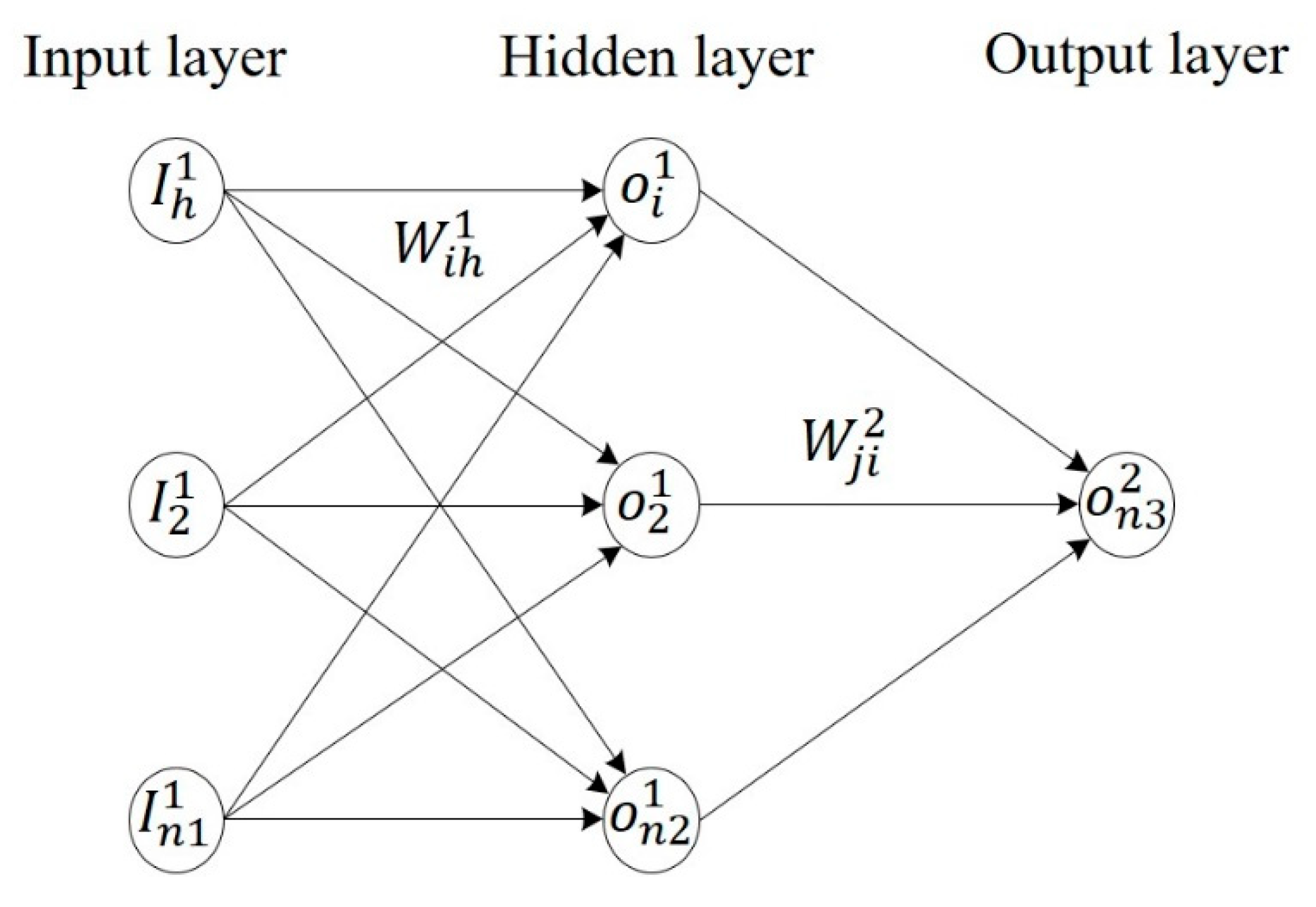
3.1. Multilayer Perceptron

Figure 2 shows the structure of a multilayer perceptron (MLP) algorithm [28]. The MLP algorithm has three layers: the input, hidden, and output layers. The input and hidden layers have three nodes and the output layer has one node in this study. The input layer passes the inputs to the hidden layer through the activation function. Then, the inputs are weighted and transferred to the nodes of the hidden layer. The hidden layer is also transferred to the output layer through the activation function. The nodes of the hidden layer are weighted and transferred to the node of the output layer.

$n1$, $n2$, and $n3$ are the respective number of nodes in each layer. The input of the input layer is ${\mathbf{I}}_{\mathrm{h}}\left(h=1,2,\cdots ,n1\right)$; then, the output of the hidden layer is expressed as

$$o_i^1=f^1\left(ne{t}_i^1\right) i=1, 2, \cdots , n2$$

(18)

where $f^1$ and $ne{t}_i^1$ are the active function and the net input of the $i$th node of the hidden layer. The net input is

$$ne{t}_i^1={\displaystyle \sum }_{h=1}^{n1}{W}_{ih}^1{I}_h+b_i^1$$

(19)

where $W_{ih}^1$ is the connection weight between the input and hidden layers and $b_i^1$ is the bias of the hidden layer. The relationship between the net input of the hidden layer and the output of the output layer is

$$o_i^2=f^2\left(ne{t}_j^2\right)j=1, 2, \cdots , n3$$

(20)

where $f^2$ and $ne{t}_j^2$ are the active function and the net input of the $j$th node of the output layer. The net input is

$$ne{t}_i^2={\displaystyle \sum }_{i=1}^{n2}{W}_{ji}^2{o}_i^1+b_j^2$$

(21)

where $W_{ji}^2$ is the connection weight between the hidden and output layers and $b_j^2$ is the bias of the output layer.

The weights and biases should be modified so that the MLP algorithm predicts the desired output. This process, the so-called learning or training, is accomplished by minimizing the error function that is defined as

$$error=\sum {\left|o_d-o_p\right|}^2$$

(22)

where $o_d$ and $o_p$ are the desired output and the predicted output.

3.2. Modal Energy and the Objective Function

The total energy ($TE\left(t\right)$) in the system adopted in the MENC algorithm can be represented by the modal parameters as

$$TE\left(t\right)={\displaystyle \sum }_{m=1}^{n}P{E}_m+{\displaystyle \sum }_{m=1}^{n}K{E}_m={\displaystyle \sum }_{m=1}^n\frac{1}{2}{k}_m^{*}{q}_m^2\left(t\right)+{\displaystyle \sum }_{m=1}^n\frac{1}{2}{m}_m^{*}{\dot{q}}_m^2\left(t\right)$$

(23)

where $P{E}_m$ and $K{E}_m$ are the $m$th modal potential and kinetic energies at time $t$, respectively; $k_m^{*}$ and $m_m^{*}$ are the modal stiffness and mass, respectively.

The modal energy is adopted in the objective function of the neuro-controller. Therefore, the objective function ($\widehat{J}$) of the proposed neuro-controller is defined as

$$\widehat{J}={\displaystyle \sum }_{k=0}^{N_f-1}\left[\mathbf{Q}\left({\mathbf{PE}}_{\mathbf{k}+1}+{\mathbf{KE}}_{\mathbf{k}+1}\right)+\frac{1}{2}{\mathbf{u}}_k^T{\mathbf{Ru}}_k\right]=\frac{1}{2}{\displaystyle \sum }_{k=0}^{N_f-1}\left[\mathbf{Q}\left({\mathbf{q}}_{k+1}^T{\mathbf{k}}^{*}{\mathbf{q}}_{k+1}+{\dot{\mathbf{q}}}_{k+1}^T{\mathbf{m}}^{*}{\dot{\mathbf{q}}}_{k+1}\right)+{\mathbf{u}}_k^T{\mathbf{Ru}}_k\right]$$

(24)

where $k$ and $N_f$ are the sampling number and the total amount of sampling time, respectively; $\mathbf{Q}$ is a set of weight factors for each mode; $\mathbf{R}$ is a weight factor for control signals; and ${\mathbf{u}}_k$ denotes the control signal. The objective function, a function of the total energy, is minimized by the control algorithm.

3.3. Control Algorithm and Training Rule

The control algorithm and training rule for the MENC algorithm are based on one of the previous neuro-controllers [6], and the proposed modal energy concept is applied to their objective function as

$$\widehat{J}=\frac{1}{2}{\displaystyle \sum }_{k=0}^{N_f-1}\left[\mathbf{Q}\left({\mathbf{q}}_{k+1}^T{\mathbf{k}}^{*}{\mathbf{q}}_{k+1}+{\dot{\mathbf{q}}}_{k+1}^T{\mathbf{m}}^{*}{\dot{\mathbf{q}}}_{k+1}\right)+{\mathbf{u}}_k^T{\mathbf{Ru}}_k\right]=\frac{1}{2}{\displaystyle \sum }_{k=0}^{N_f-1}{\widehat{J}}_k .$$

(25)

By applying the gradient descent rule to the objective at the $k$th step, the update for the weight, ${\mathbf{W}}_{ji}^2$, at the $k$th step can be expressed as

$$\mathsf{\Delta }{\mathrm{W}}_{ji}^2=-\eta \frac{\partial {\widehat{J}}_k}{\partial W_{ji}^2}$$

(26)

where $\eta$ is the learning rate. The objective function is made to converge by varying the rate. Using the chain rule, the partial derivative of Equation (26) can be rewritten as

$$\frac{\partial {\widehat{J}}_k}{\partial W_{ji}^2}=\frac{\partial {\widehat{J}}_k}{\partial ne{t}_j^2}\frac{\partial ne{t}_j^2}{\partial W_{ji}^2}.$$

(27)

Assuming that the general error is the same as Equation (28), the weight update of the output layer can be simply expressed as Equation (29)

$${\delta }_j^2=-\frac{\partial {\widehat{J}}_k}{\partial ne{t}_j^2}=-\frac{\partial {\widehat{J}}_k}{\partial o_j^2}\frac{\partial o_j^2}{\partial ne{t}_j^2}$$

(28)

$$\mathsf{\Delta }{W}_{ji}^2=\eta {\delta }_j^2{o}_i^1$$

(29)

where

$${\delta }_j^2=\left[\left\{{\left({\mathbf{k}}^{*}{\mathbf{q}}_{k+1}\right)}^T\mathbf{Q}\frac{\partial {\mathbf{q}}_{k+1}}{\partial {\mathbf{u}}_k}+{\left({\mathbf{m}}^{*}{\dot{\mathbf{q}}}_{k+1}\right)}^T\mathbf{Q}\frac{\partial {\dot{\mathbf{q}}}_{k+1}}{\partial {\mathbf{u}}_k}\right\}+{\mathbf{u}}_k^T\mathbf{R}\right]G_j{\left(f^2\right)}^{\prime }{|}_{ne{t}_j^2}$$

(30)

The bias is also updated using Equation (31).

$$\mathsf{\Delta }{b}_j^2=\eta {\delta }_j^2$$

(31)

In Equation (30), the gain factor satisfying $u_j=G_j{o}_j^2$ and ${\left(f^2\right)}^{\prime }{|}_{ne{t}_j^2}$ denotes the derivation of the activation function on the $ne{t}_j^2$ in the output layer; $\left[\partial {\mathbf{q}}_{k+1}/\partial {\mathbf{u}}_k \partial {\dot{\mathbf{q}}}_{k+1}/\partial {\mathbf{u}}_k\right]$ is the sensitivity that is calculated by the structural response after applying the unit control signal during one sampling period.

In the same manner, an update for the weight between the input and hidden layers can be obtained as

$$\mathsf{\Delta }{W}_{ih}^1=\eta {\delta }_i^1{I}_h$$

(32)

where

$${\delta }_i^1=-\frac{\partial {\widehat{J}}_k}{\partial ne{t}_i^1}={\displaystyle \sum }_{j=1}^{n3}\frac{\partial {\widehat{J}}_k}{\partial ne{t}_j^2}\frac{\partial ne{t}_j^2}{\partial o_i^1}\frac{\partial o_i^1}{\partial ne{t}_i^1}={\displaystyle \sum }_{j=1}^{n3}{\delta }_j^2{W}_{ji}^2{\left(f^1\right)}^{\prime }{|}_{ne{t}_i^1}.$$

(33)

The bias of the hidden layer is updated using Equation (34).

$$\mathsf{\Delta }{b}_j^1=\eta {\delta }_i^1$$

(34)

4. Numerical Analysis

To verify the effectiveness of the MENC algorithm, a three-story building was installed with the AMD (in Figure 1), which was used to reduce the response of the structure under seismic load. The structural properties and simulation parameters of the previous neuro-controller system were used to compare its capabilities [6]. The parameters of the structure and AMD system are shown in

Table 1. Structural model parameters of the AMD device control [6].

Symbol	Quantity	Value
$m_i$	Mass of each floor	200 kg
$m_a$	Mass of AMD	18 kg
$k_i$	Stiffness coefficient of each floor	2.25 × 105 N/m
${\xi }_1$	Damping ratio of first mode	0.6%
${\xi }_2$	Damping ratio of second mode	0.7%
${\xi }_3$	Damping ratio of third mode	0.3%
$g_1$	Valve gain	321.4 × 102 m3/s
$g_2$	Valve gain	0.28 × 10−6 m3/s
$\tau$	Time constant	0.1
$a_r$	Piston effective area	1.52 × 10−3 m2
$V$	Volume of the cylinder	4.56 × 10−4 m3
$c_l$	Leakage coefficient	1.0 × 10−11
$\beta$	Compressibility coefficient	2.1 × 109
$\alpha$	Contribution to restoring force (for nonlinear)	0.5
$d$	Constant (for nonlinear)	0.01
$\rho$	Constant of hysteretic behavior	1.0
$\mu$	Constant of hysteretic behavior	0.5
$\sigma$	Constant of hysteretic behavior	0.5
$p$	Constant of hysteretic behavior	5

. The sampling time was 0.005 s, and the delay time was assumed to be 0.0005 s. The equation of motion was integrated at every 0.00025 s using MATLAB/Simulink software. The MENC algorithm is used to calculate the accurate control command to be exerted on the AMD system.

4.1. Training the Neuro-Controller

For the simulation of the MENC algorithm, the input layer has three nodes: the displacement, the acceleration of the third floor, and the ground acceleration. Here, the displacement was calculated by integrating the acceleration, and the modal energy for each mode was used for training the MENC algorithm. The hidden layer has three nodes. The output layer has one node, which is the control signal. The tan-sigmoid function was used as the activation function of the hidden layer and output layer. The control signal was normalized to the maximum assumed output voltage, which was 3 volts.

The weight factors for each mode were ${\mathbf{Q}}_1=0.9042$, ${\mathbf{Q}}_2=0.0089$, and ${\mathbf{Q}}_3=0.0867$, respectively, in the objective function (in Equation (25)). The weight factor of the first mode was determined by the largest value due to the modal participating factor. The mode shape of the building was used to calculate the modal energy. The El Centro earthquake, one of the most famous earthquakes, was selected for the training of the MENC algorithm. Considering the repetitive training time, the 10-second range with a lot of energy of the El Centro earthquake (1940) were used for the training data (see Figure 3). Training was repeated 200 times. The histories of the objective functions of the MLP and MENC algorithm are shown in Figure 4. It can be seen that the objective function of the proposed MENC algorithm converged faster than did that of the MLP algorithm. In other words, the proposed MENC algorithm is faster than the MLP algorithm in the training process.

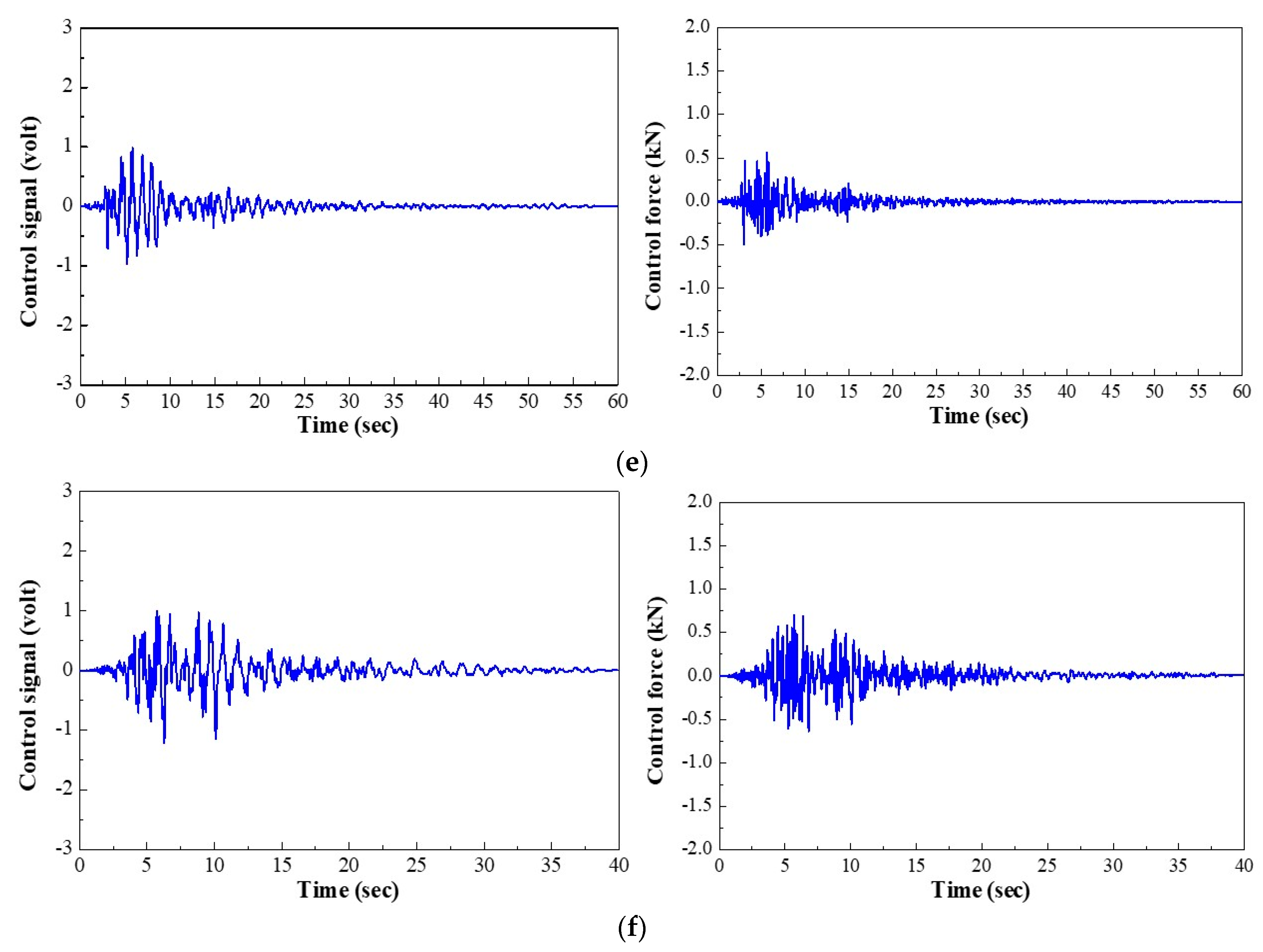
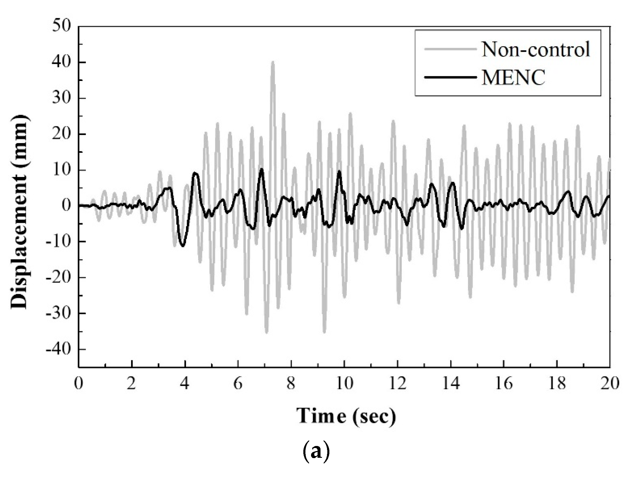
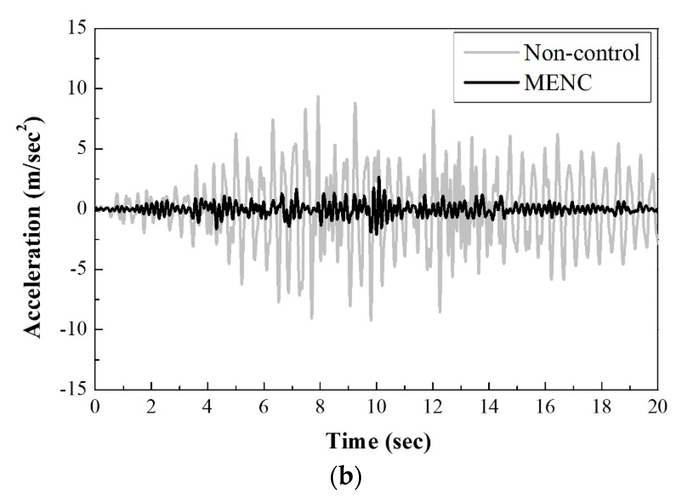
4.2. Comparison of Control Results

The California, Northridge, Landers, Cape, San Simeon, and Loma Prieta earthquakes obtained from PEER Center [29] were used to verify the proposed algorithm regarding nonlinear building structures under seismic loads after training (see Figure 5). Figure 6 shows a comparison of the results of controlled response on the third floor of the building using MLP and MENC. Compared with MLP, the decreasing rate of the maximum displacement by the MENC algorithm is shown in

Table 2. Comparison of the maximum displacement at the third floor according to the algorithms applied to the AMD system under seismic loads (MLP vs. MENC).

	MLP Algorithm	MENC Algorithm	Decreasing Rate
California earthquake	23.20 mm	11.17 mm	51.84%
Northridge earthquake	30.54 mm	17.31 mm	43.32%
Landers earthquake	14.89 mm	6.72 mm	54.83%
Cape earthquake	14.15 mm	9.04 mm	36.09%
San Simeon earthquake	7.92 mm	6.60 mm	16.77%
Loma Prieta earthquake	12.56 mm	6.34 mm	49.55%

. Comparison results of the MLP and MENC algorithms showed the maximum displacement reduction rate (54.83%) under the Landers earthquake and the minimum displacement reduction rate (16.77%) under the San Simeon earthquake. Therefore, it was found that the proposed MENC algorithm is able to effectively reduce the structural responses under unknown earthquakes than conventional MLP.

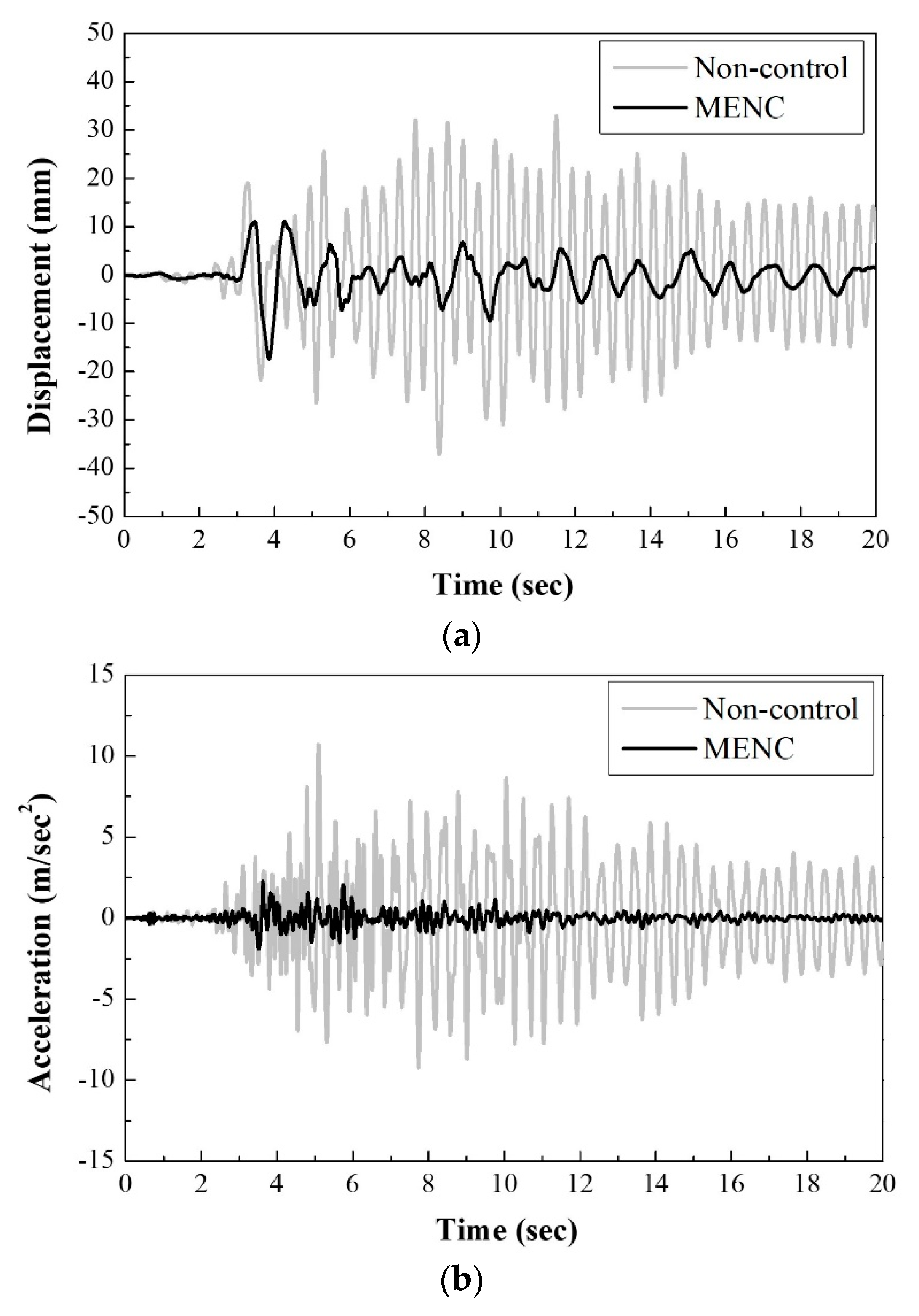
4.3. Numerical Analysis of Nonlinear Building Structures

Figure 7 shows the control signal and control force exerted on the structure by the AMD during the seismic loads, respectively.

Figure 8 and Figure 9 show the responses (displacement and acceleration) to control and non-control of the nonlinear building structure by the proposed MENC algorithm in the event of the California earthquake and the Northridge earthquake, respectively. The California earthquake and the Northridge earthquake were not used in the training.

The decreasing rate of the maximum responses on the seismic loads is also shown in

Table 3. Comparison of the maximum responses in control and non-control of the building structure under the seismic loads.

	Max. Displacement (mm)			Max. Acceleration (m/s2)
	Non-Control	Control by MENC	Decreasing Rate	Non-Control	Control by MENC	Decreasing Rate
California earthquake	40.10	11.17	72.14%	9.38	2.66	71.64%
Northridge earthquake	37.06	17.31	53.29%	10.71	2.29	78.62%
Landers earthquake	28.11	6.73	76.06%	7.39	1.62	78.09%
Cape earthquake	28.85	9.04	68.67%	8.23	1.85	77.52%
San Simeon earthquake	25.96	6.60	74.58%	7.12	0.82	88.48%
Loma Prieta earthquake	28.97	6.34	78.12%	7.12	1.08	84.83%

. The decreasing rates of the maximum displacement and acceleration on the third floor were 78.12% and 88.48%, respectively. Therefore, it was found that the proposed MENC algorithm could significantly reduce the structural response under unknown seismic load if applied to the AMD system.

The modal energies of the nonlinear building structures during the California and Northridge earthquakes are shown in Figure 10 and Figure 11, respectively. The total energy, including the modal energy and the control energy of the building during both earthquakes, was remarkably reduced through the proposed MENC algorithm. Also, it was found that the first modal energy affected the whole structure’s energy because the first mode is dominant in this structure’s case. The total modal energy of the nonlinear building structure during the remaining four earthquakes is shown in Figure 12.

Figure 13 shows the relationships between the restoring force and the displacement on the first floor of the building structure caused by the seismic loads. Figure 13 also shows the non-controlled and controlled responses caused by the seismic loads, indicating that the target structure behaved nonlinearly. Differently from linear structures which have constant stiffness, nonlinear structures need to establish the structural restoring force model to determine its stiffness at every moment [30]. If the structural displacement is greater than the structural yield displacement, the structure enters the plastic range. While nonlinear hysteretic behaviors appeared in the non-control responses, this nonlinear behavior almost entirely disappeared after control under all earthquakes.

5. Conclusions

A modal-energy-based neuro-controller (MENC) algorithm was presented to reduce structural vibration under seismic load. The applicability of the presented control algorithm was demonstrated through numerical analysis. A three-story nonlinear building was installed with an active mass damper, which was used to verify the applicability of the proposed control algorithm. The El Centro earthquake was adopted to train the modal-energy-based neuro-controller. Six recorded earthquakes obtained from PEER center [29] were employed to consider unknown earthquakes effects after training. The results of the proposed control algorithm were compared with those obtained from a non-controlled response and a multilayer perceptron (MLP). The key observations and findings of this research can be summarized as follows:

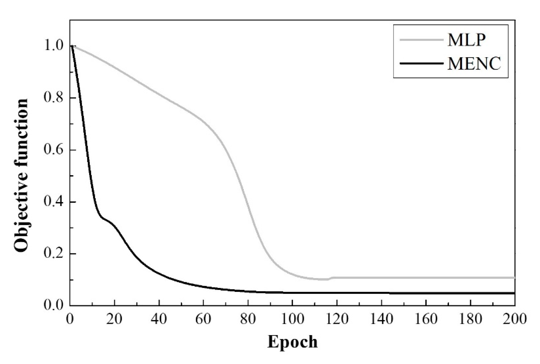
• The proposed MENC algorithm was faster compared to the MLP algorithm in the training process to control the seismic load of an active mass damper.
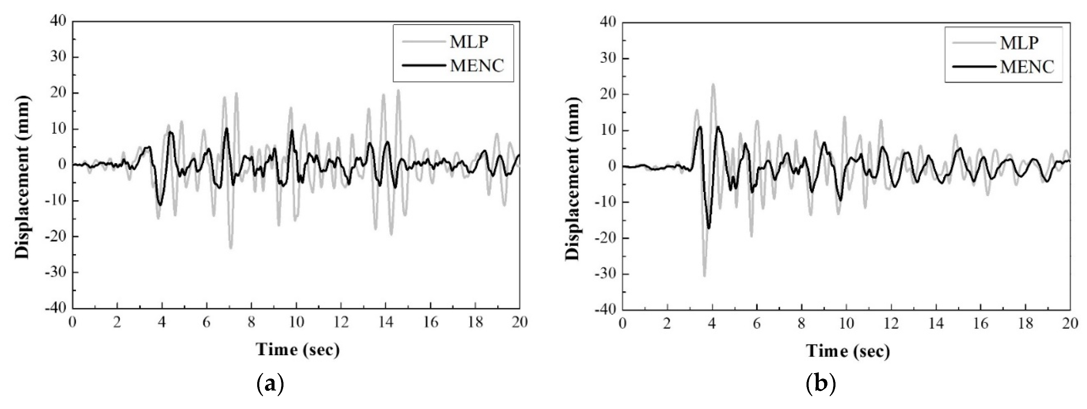
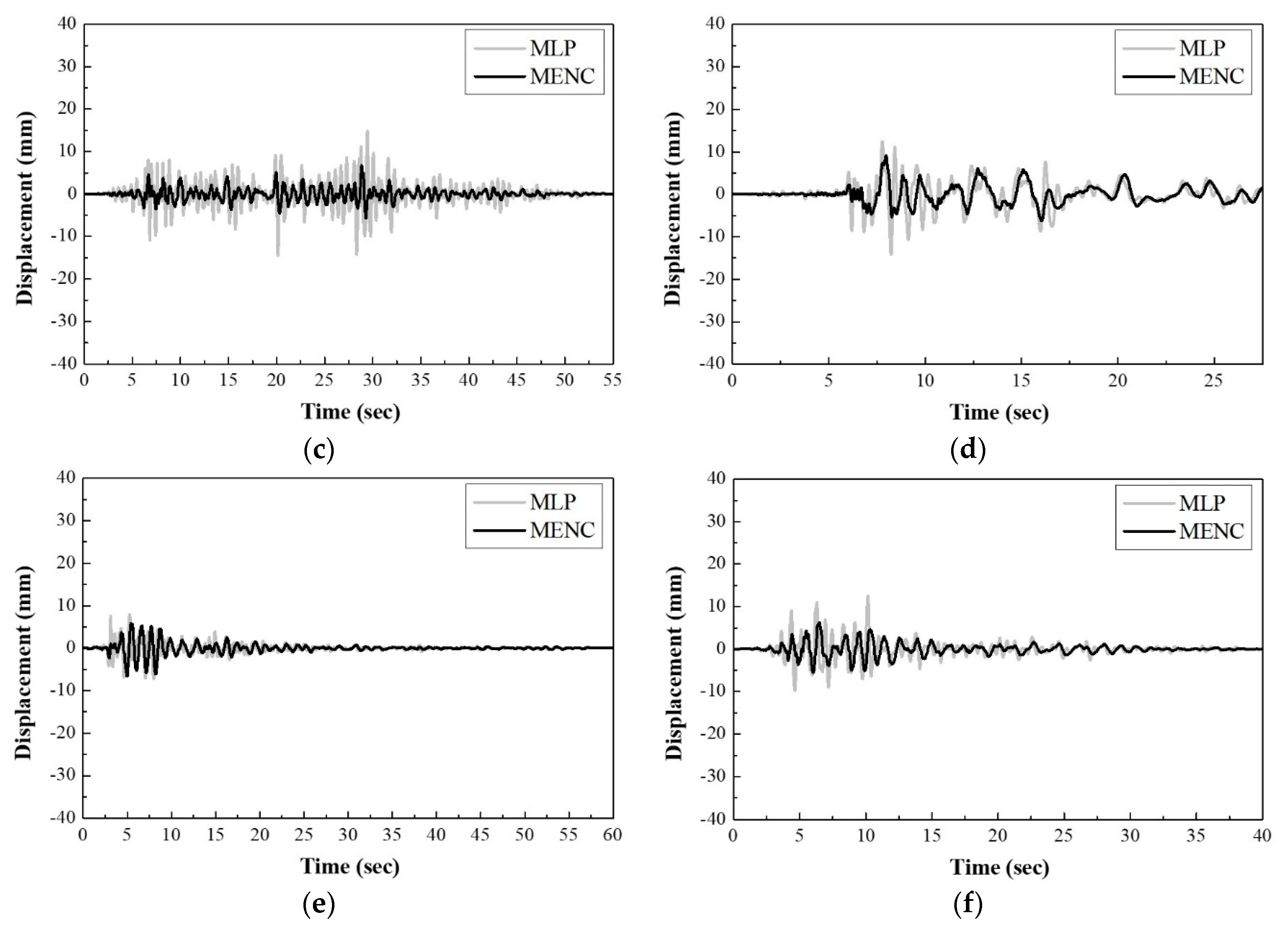
• The proposed MENC algorithm is able to effectively reduce the structural responses under unknown earthquakes than conventional MLP.
• The proposed MENC algorithm was able to significantly reduce the structural response under all used seismic loads when applied to an AMD system.
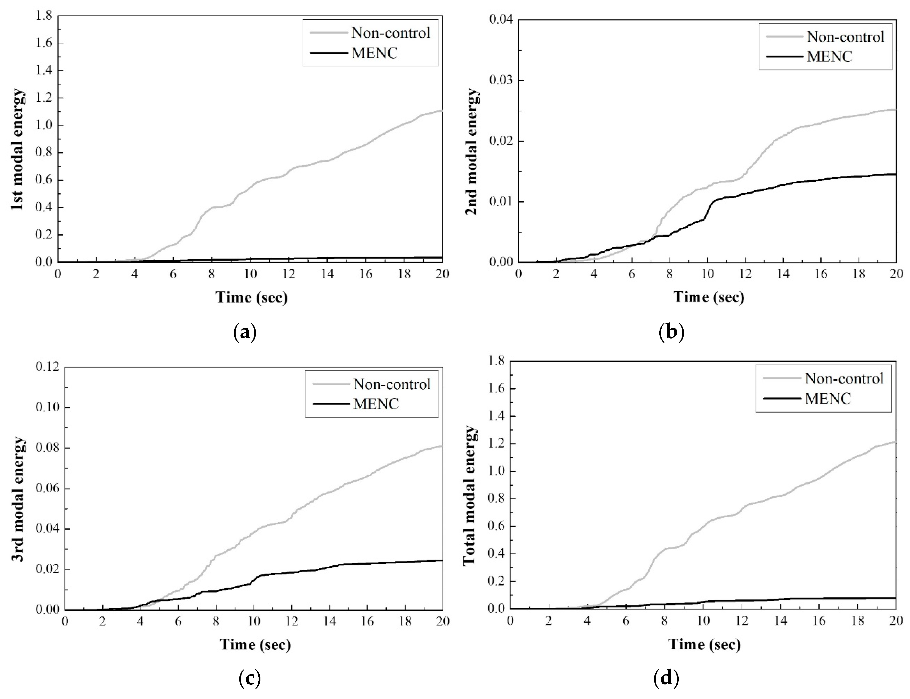
• The structural responses and modal energy were suppressed effectively by the MENC algorithm. In addition, the first modal energy affected the whole structure’s energy because the first mode is dominant in this structure’s case.
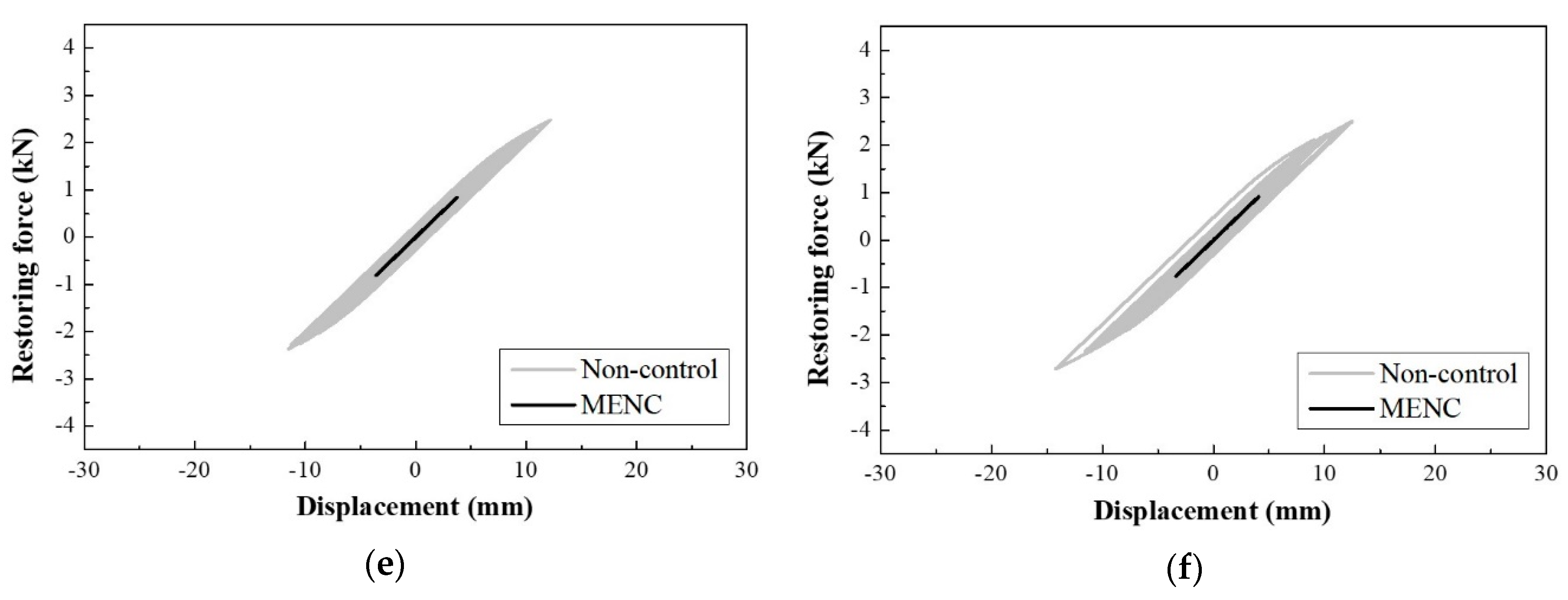
• From the restoring force results, the non-controlled structural responses exhibited nonlinear hysteretic behaviors. This nonlinear behavior almost disappeared after control by the proposed MENC algorithm. Therefore, when the structure is in the nonlinear state, the proposed MENC algorithm can effectively reduce the seismic response by the control signal in real time depending on the structural responses.

This algorithm should be considered in future experimental research in order to achieve more practical vibration control of nonlinear building structures under seismic loads. In addition, it is necessary to suggest the possibility of applying the proposed vibration control algorithm to other electric power systems [31] and offshore wind turbines [32].

References

1. Chen, H.M.; Tsai, K.H.; Qi, G.Z.; Yang, C.S.; Amini, F. Neural network for structure control. J. Comput. Civ. Eng. 1995, 9, 168–176. [Google Scholar] [CrossRef]
2. Ghaboussi, J.; Joghataie, A. Active control of structure using neural networks. J. Eng. Mech. ASCE 1995, 121, 555–567. [Google Scholar] [CrossRef]
3. Bani-Hani, K.; Ghaboussi, J. Nonlinear structural control using neural networks. J. Eng. Mech. ASCE 1998, 124, 319–328. [Google Scholar] [CrossRef]
4. Bani-Hani, K.; Ghaboussi, J. Neural networks for structural control of a benchmark problem, active tendon system. Earthq. Eng. Struct. D 1998, 27, 1225–1245. [Google Scholar] [CrossRef]
5. Liut, D.A.; Matheu, E.E.; Singh, M.P.; Mook, D.T. Neural-network control of building structures by a force-matching training scheme. Earthq. Eng. Struct. D 1999, 28, 1601–1620. [Google Scholar] [CrossRef]
6. Kim, D.H.; Lee, I.W. Neuro-control of seismically excited steel structure through sensitivity evaluation scheme. Earthq. Eng. Struct. D 2001, 30, 1361–1377. [Google Scholar] [CrossRef]
7. Cho, H.C.; Fadali, M.S.; Saiidi, M.S.; Lee, K.S. Neural network active control of structures with earthquake excitation. Int. J. Control Autom. 2005, 3, 202–210. [Google Scholar]
8. Madan, A. Vibration control of building structures using self-organizing and self-learning neural networks. J. Sound Vib. 2005, 287, 759–784. [Google Scholar] [CrossRef]
9. Lee, H.J. Neural Network-Based Structural Vibration Control System. Ph.D. Thesis, Korea Advanced Institute of Science and Technology, Daejeon, Korea, 2007. [Google Scholar]
10. Lewis, A.D. The Maximum Principle of Pontryagin in Control and in Optimal Control; Queen’s University: Kingston, ON, Canada, 2006. [Google Scholar]
11. Jakubczyk, B.; Sontag, E. Controllability of nonlinear discrete-time systems: A lie-algebraic approach. SIAM J. Control Optim. 1990, 28, 1–33. [Google Scholar] [CrossRef]
12. Mardanov, M.J.; Sharifov, Y.A. Pontryagin’s maximum principle for the optimal control problems with multipoint boundary conditions. Abstr. Appl. Anal. 2015, 2015, 1–6. [Google Scholar] [CrossRef]
13. Greydanus, S.; Dzamba, M.; Yosinski, J. Hamiltonian neural networks. arXiv 2019, arXiv:1906.01563. [Google Scholar]
14. Zhong, Y.D.; Dey, B.; Chakraborty, A. Symplectic ODE-Net: Learning Hamiltonian dynamics with control. arXiv 2019, arXiv:1909.12077. [Google Scholar]
15. Zizouni, K.; Fali, L.; Sadek, Y.; Bousserhane, I.K. Neural network control for earthquake structural vibration reduction using MRD. Front. Struct. Civ. Eng. 2019, 9, 1171–1182. [Google Scholar] [CrossRef]
16. Rodríguez, A.; Pozo, F.; Bahar, A. Force-derivative feedback semi-active control of base-isolated buildings using large-scale MR fluid dampers. Struct. Control Health 2012, 19, 120–145. [Google Scholar] [CrossRef]
17. Bharti, S.; Dumne, S.; Shrimali, M. Earthquake response of asymmetric building with MR damper. Earthq. Eng. Eng. Vib. 2014, 13, 305–316. [Google Scholar] [CrossRef]
18. Gattulli, V.; Lepidi, M.; Potenza, F. Seismic protection of frame structures via semi-active control: Modeling and implementation issues. Earthq. Eng. Eng. Vib. 2009, 8, 627–645. [Google Scholar] [CrossRef]
19. Oliveira, F.; Botto, M.A.; Morais, P.; Suleman, A. Semi-active structural vibration control of base-isolated buildings using magnetorheological dampers. J. Low Freq. Noise Vib. Act. Control 2017, 37, 565–576. [Google Scholar] [CrossRef]
20. Fu, W.; Zhang, C.; Li, M.; Duan, C. Experimental investigation on semi-active control of base isolation system using magnetorheological dampers for concrete frame structure. Appl. Sci. 2019, 9, 3866. [Google Scholar] [CrossRef]
21. Demetriou, D.; Nikitas, N. A novel hybrid semi-active mass damper configuration for structural applications. Appl. Sci. 2016, 6, 397. [Google Scholar] [CrossRef]
22. Ma, X.; Wang, L.; Xu, J. Active vibration control of rib stiffened plate by using decentralized velocity feedback controllers with inertial actuators. Appl. Sci. 2019, 9, 3188. [Google Scholar] [CrossRef]
23. Lin, Y. Semi-Active Structural Motion Control by Transfer of Modal Energy. Ph.D. Thesis, University of Texas, Austin, TX, USA, 1994. [Google Scholar]
24. Emad, N.A. Acceleration Behavior of Semi-Active Structural Motion Control by Transfer of Modal Energy. Master’s Thesis, University of Texas, Austin, TX, USA, 1996. [Google Scholar]
25. Benavent-Climent, A.; Morillas, L.; Escolano-Margarit, D. Seismic performance and damage evaluation of a reinforced concrete frame with hysteretic dampers through shake-table tests. Earthq. Eng. Struct. D 2014, 43, 2399–2417. [Google Scholar] [CrossRef] [Green Version]
26. Enrıquez-Zarate, J.; Abundis-Fong, H.F.; Velazquez, R.; Gutierrez, S. Passive vibration control in a civil structure: Experimental results. Meas. Control 2019, 52, 938–946. [Google Scholar] [CrossRef]
27. Baber, T.T.; Wen, Y.K. Random vibration of hysteretic degrading systems. J. Eng. Mech. Div. ASCE 1981, 107, 1069–1087. [Google Scholar]
28. Rumelhart, D.E.; Geoffrey, E.H.; Williams, R.J. Learning Internal Representations by Error Propagation; ICS Report; MIT Press: Cambridge, MA, USA, 1986. [Google Scholar]
29. Pacific Earthquake Engineering Research Center. Available online: https://ngawest2.berkeley.edu/site (accessed on 11 October 2019).
30. Tu, J.; Lin, X.; Tu, B.; Xu, J.; Tan, D. Simulation and experimental tests on active mass damper control system based on model reference adaptive control algorithm. J. Sound Vib. 2014, 333, 4826–4842. [Google Scholar] [CrossRef]
31. Wang, C.; Feng, K.; Zhang, H.; Li, Q. Seismic performance assessment of electric power systems subjected to spatially correlated earthquake excitations. Struct. Infrastruct. E 2019, 15, 351–361. [Google Scholar] [CrossRef]
32. Plodpradit, P.; Dinh, V.N.; Kim, K.D. Coupled Analysis of Offshore Wind Turbine Jacket Structures with Pile-Soil-Structure Interaction Using FAST v8 and X-SEA. Appl. Sci. 2019, 9, 1633. [Google Scholar] [CrossRef]
Figure 1. Idealized schematic diagram of a three-story building structure with an active mass damper (AMD).
Applsci 09 04443 g001
Figure 2. Structure of a multilayer perceptron (MLP) algorithm.
Applsci 09 04443 g002
Figure 3. El Centro earthquake for training.
Applsci 09 04443 g003
Figure 4. History of objective functions during training.
Applsci 09 04443 g004
Figure 5. Seismic loads for the numerical analysis: (a) California earthquake; (b) Northridge earthquake; (c) Landers earthquake; (d) Cape earthquake; (e) San Simeon earthquake; (f) Loma Prieta earthquake.
Applsci 09 04443 g005
Figure 6. Time-histories of structural displacement response under different control algorithms: (a) California earthquake; (b) Northridge earthquake; (c) Landers earthquake; (d) Cape earthquake; (e) San Simeon earthquake; (f) Loma Prieta earthquake.
Applsci 09 04443 g006aApplsci 09 04443 g006b
Figure 7. Control signal and control force of the AMD system under the seismic loads: (a) California earthquake; (b) Northridge earthquake; (c) Landers earthquake; (d) Cape earthquake; (e) San Simeon earthquake; (f) Loma Prieta earthquake.
Applsci 09 04443 g007aApplsci 09 04443 g007b
Figure 8. Comparison of control and non-control responses of the building structure under the California earthquake: (a) displacement; (b) acceleration.
Applsci 09 04443 g008aApplsci 09 04443 g008b
Figure 9. Comparison of control and non-control responses of the building structure under the Northridge earthquake: (a) displacement; (b) acceleration.
Applsci 09 04443 g009
Figure 10. Comparison of modal energies in the control and non-control of the building structure under the California earthquake: (a) first modal energy; (b) second modal energy; (c) third modal energy; (d) total modal energy.
Applsci 09 04443 g010
Figure 11. Comparison of modal energies in the control and non-control of the building structure under the Northridge earthquake: (a) first modal energy; (b) second modal energy; (c) third modal energy; (d) total modal energy.
Applsci 09 04443 g011
Figure 12. Comparison of total modal energy in the control and non-control of the building structure under the seismic load: (a) Landers earthquake; (b) Cape earthquake; (c) San Simeon earthquake; (d) Loma Prieta earthquake.
Applsci 09 04443 g012aApplsci 09 04443 g012b
Figure 13. Restoring force vs. displacement on the first floor under the seismic load: (a) California earthquake; (b) Northridge earthquake; (c) Landers earthquake; (d) Cape earthquake; (e) San Simeon earthquake; (f) Loma Prieta earthquake.
Applsci 09 04443 g013aApplsci 09 04443 g013b