Article

Rolling Bearing Incipient Fault Detection Based on a Multi-Resolution Singular Value Decomposition

1
School of Mechanical and Automotive Engineering, Xiamen University of Technology, Xiamen 361024, China
2
Key Laboratory of Precision Actuation and Transmission, Fujian Province University, Xiamen 361024, China
3
College of Mechanical Engineering, Dongguan University of Technology, Dongguan 523808, China
*
Author to whom correspondence should be addressed.
Appl. Sci. 2019, 9(20), 4465; https://doi.org/10.3390/app9204465
Submission received: 9 September 2019 / Revised: 16 October 2019 / Accepted: 17 October 2019 / Published: 22 October 2019
(This article belongs to the Section Mechanical Engineering)

Abstract

:
The periodic impulse characteristics caused by rolling bearing damage are weak in the incipient failure stage. Thus, these characteristics are always drowned out by background noise and other harmonic interference. A novel approach based on multi-resolution singular value decomposition (MRSVD) is proposed in order to extract the periodic impulse characteristics for incipient fault detection. With the MRSVD method, the vibration signal is first decomposed to obtain a group of approximate signals and detailed signals with different resolutions. The first detail signal is mainly composed of noise and the last approximate signal is mainly composed of harmonic interference. Combined with the kurtosis index, the hidden periodic impulse signal will be extracted from the detail signals (in addition to the first detail signal). Thus, the incipient fault detection of a rolling bearing can be fulfilled according to the envelope demodulation spectrum of the extracted periodic impulse signal. The effectiveness of the proposed method has been demonstrated with both simulation and experimental analyses.

1. Introduction

When a rolling bearing has a local injury in addition to its periodic rotation, the damaged surface will be in contact with other parts that can produce periodic pulse impact, and thus arouse the natural frequency vibration of the inner and outer rings [1,2]. The periodic transient shock signal often occurs in the vibration signal and forms the modulation phenomenon, which is manifested in the frequency spectrum as a modulated side band with equal intervals on both sides of the natural frequency [1,3]. Therefore, vibration signals collected from rolling bearings always carry the rich information about machine health conditions [4,5,6]. Hence, the vibration-based fault detection methods have received intensive study during the past decades.
In order to extract the fault feature information from vibration signals, various signal processing methods have been used in the field of fault detection [7,8], such as empirical mode decomposition (EMD) [9], wavelet transform (WT) [10], and their improved methods [11,12,13,14], sparse decomposition [15,16], manifold learning [17], deep learning [18], spectral kurtosis(SK) [19], and envelope analysis [20,21,22,23,24]. These methods realize fault detection from the time domain, frequency domain, or time–frequency domain. In addition to the above methods, there is another kind of method that has been universally used for bearing fault detection to certain success, that is, higher order spectral (HOS) analysis [25,26,27,28,29,30,31,32,33]. HOS methods such as bispectrum, third order spectrum, etc, were put forward to compensate for the deficiencies of the FFT(Fast Fourier Transform Algorithm)-based techniques when they process the non-stationary and non-Gaussian signals. HOS methods realize fault detection from higher-order spectral domains. No matter which domain is selected for bearing fault detection, the objective of the above methods is the detection of the modulation phenomenon formed by the periodic shock characteristics in the resonance band that is excited by the bearing faults, i.e., the resonant demodulation. The reasonable selection of the resonance band will promote the fault detection accuracy of the above methods. However, due to the existence of the background noise and harmonic vibrations in the initial stage of the failure, it is usually difficult to select the optimal frequency band for resonant demodulation. Therefore, the effectiveness of the above resonance demodulation methods is undermined.
Some signal processing methods are applied in order to preprocess the raw vibration signals [12,34,35,36]. Chibani et al. [37] designed a novel filter in the finite frequency range to overcome the conservatism generated. Chadli et al. [38] proposed a novel fault detection and isolation filter for multi-agent systems. Based on GKYP(generalised Kalman–Yakubovich–Popov) lemma, Zhu et al. [39] proposed a filter to detect faults for vehicle active suspension systems. Li et al. [40] developed a weighted diagnostic observer to optimize the worst case robustness and fault sensitivity simultaneously. The purpose of the preprocessing is to remove the noise and harmonic interference and extract the periodic shock vibration components that are related to the fault for demodulation analysis. In essence, these preprocessing methods decompose the background noise, the harmonic interference, and the periodic shock vibration into different frequency bands. Therefore, the background noise, the harmonic interference, and the periodic shock vibration that are contained in the raw vibration signal should be separable in the frequency domain.
Different types of signals have different singular value characteristics after the singular value decomposition (SVD). Therefore, SVD-based signal processing methods have been proposed, either for noise reduction or classification recognition. The SVD based methods have been also widely used for bearings and rotor-related fault detection to certain success [41,42,43,44,45]. The background noise, the harmonic interference, and the periodic shock vibration have different singular value characteristics after the singular value decomposition (SVD). In contrast to the above frequency-separation-based methods, a new SVD-based preprocessing method, that is, multi-resolution singular value decomposition (MRSVD) [46], is introduced in this study with the objective of extracting the periodic shock vibration from the raw vibration signal which is acquired at the incipient failure stage of a rolling bearing.
Multi-resolution singular value decomposition (MRSVD) is a new signal decomposition method that has been proposed in recent years. Inspired by the multi-resolution analysis idea of wavelet analysis and the construction principle of matrix dichotomy recursion, MRSVD decomposes the analytic signal into a number of approximate and detail signals with different resolutions via the SVD method. As shown in the theoretical analysis in Section 3.1, in the MRSVD decomposition results of a mixed-signal that contains strong background noise, harmonic disturbances, and a periodic shock vibration, the first detail signal is mainly composed of noise, and the last approximate signal is mainly composed of harmonic disturbances. Therefore, the MRSVD method is used to preprocess the rolling bearing vibration signal to remove the background noise signal and the harmonic interference signal. The simulation analysis and the application examples show that the MRSVD method can effectively extract the periodic impact components caused by a bearing fault, even under the influence of strong background noise and harmonic disturbances. Furthermore, the proposed method does not require any prior knowledge about the resonance band. Hence, the MRSVD method has a good application prospect for the initial fault detection of a rolling bearing.

2. Overview of the Method of Multi-Resolution Singular Value Decomposition

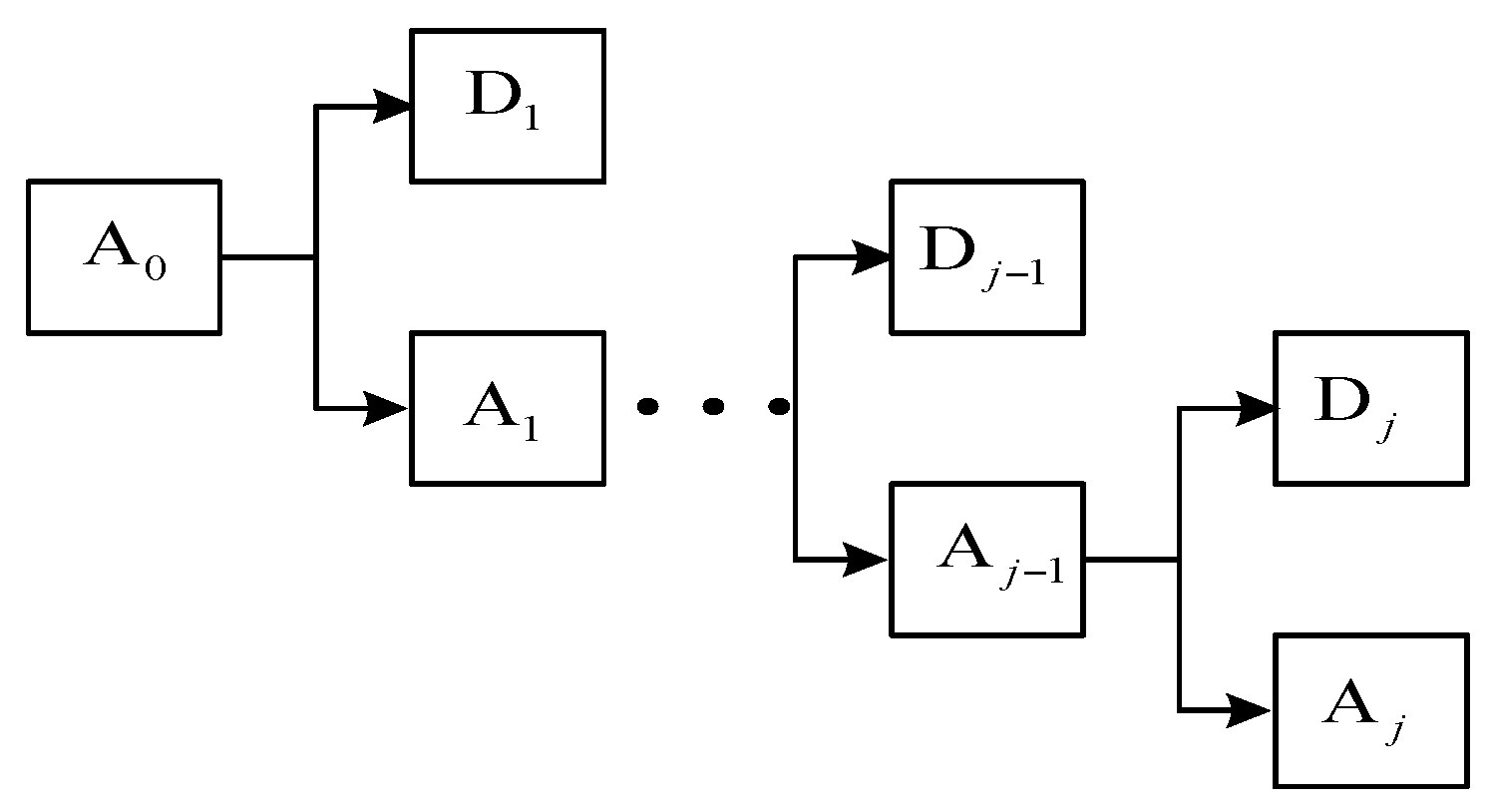
2.1. Decomposition Process of MRSVD

Inspired by the multi-resolution analysis idea of wavelet analysis and the construction principle of matrix dichotomy recursion, a new SVD-based method that is MRSVD is proposed [46]. The specific steps of the algorithm are as follows and the decomposition process is shown in Figure 1.
Step 1. A Hankel matrix H0 is constructed with two rows for a given signal A0 = (x1, x2, … xN), i.e., H 0 = ( x 1 , x 2 , , x N 1 x 2 , x 3 , , x N ) .
Step 2. An SVD is performed on the matrix H0, and on the two obtained singular values that are denoted as σa1 and σd1, with σa1 > σd1. Two signal components can be obtained from σa1 and σd1 via the principle of the SVD matrix’s dichotomy recursive algorithm (see the Section 2.2), and these two signal components are denoted as A1 and D1. In terms of the contribution to the original signal, A1 and D1 have different weights. The A1 signal has a larger contribution to the original signal. It is the main component of the original signal and it reflects the main profile obtained from the original signal during the current signal decomposition. Similar to the approximate signal in wavelet analysis, the A1 signal is called as SVD approximate signal. In addition, the D1 signal reflects the details obtained from the original signal during the current signal decomposition. The D1 signal is similar to the detail signal in the wavelet analysis, so it is called the SVD detail signal.
Step 3. The detail signal D1 is preserved, and the construction of the 2-row Hankel matrix H1 is continued for the A1 approximate signal in order to obtain the next level singular value decomposition. Consequently, a series of SVD detail signals and approximate signals can be obtained using the recursion decomposition layer by layer.

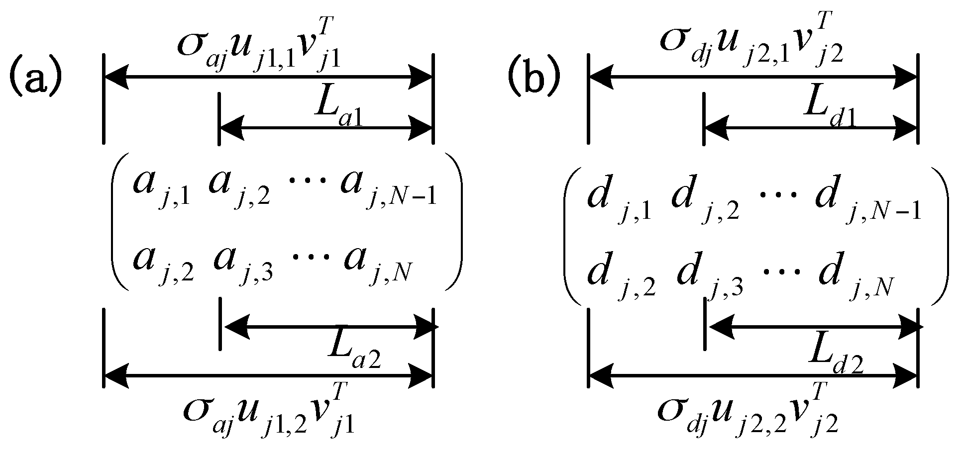
2.2. Principle of the SVD Matrix’s Dichotomy Recursive Algorithm

Presuming that the (j−1)th MRSVD decomposition of the given signal A0 = (x1, x2, … xN) has been carried out, the (j−1)th SVD approximate signal will have also been obtained and denoted as Aj−1 = (aj−1,1, aj−1,2, … n aj−1,N). A 2-row Hankel matrix Hj can be constructed, i.e., H j = ( a j 1 , 1 , a j 1 , 2 , , a j 1 , N 1 x j 1 , 2 , x j 1 , 3 , , x j 1 , N ) .
The SVD result of the matrix Hj can be expressed as
Hj = Uj SjVj
where Uj = (uj1, uj2), Uj ∈ R2×2, Vj = (vj1, vj2, …, vj(N−1)), Vj ∈ R(N−1)×(N−1), and Uj and Vj are the left and right orthogonal matrices obtained by the jth decomposition. Sj = (diag(σaj, σdj), 0), Sj ∈ R2×(N−1), and σaj and σdj are the approximate singular value and the detail singular value obtained using the jth decomposition.
In order to obtain the SVD approximate signal Aj and the detail signal Dj for the jth decomposition, Hj in the formula (1) can be expressed as the following form.
H j = σ a j u j 1 v j 1 T + σ d j u j 2 v j 2 T
where uj1 ∈ R2×1, vj1 ∈ R(N−1)×1, and i = 1,2. Denoting H a j = σ a j u j 1 v j 1 T , then Haj ∈ R2×(N−1) and Haj corresponds to the larger singular value σaj, which reflects the body of the original signal, so it is called the approximation matrix. In addition, H d j = σ d j u j 2 v j 2 T , Hdj ∈ R2×(N−1), and Hdj corresponds to the smaller singular value σd, which reflects the detail of the original signal, so it is called the detail matrix. The SVD approximate signal Aj and the detail signal Dj are obtained from Haj and Hdj, respectively, and the specific process is described as follows.
Both of the matrixes, Haj and Hdj, can be expressed in the form of row vectors, i.e., H a j = ( σ a j u j 1 , 1 v j 1 T σ a j u j 1 , 2 v j 1 T ) and H d j = ( σ d j u j 2 , 1 v j 2 T σ d j u j 2 , 2 v j 2 T ) . The specific row vector forms of the Haj and Hdj matrixes are displayed in Figure 2a,b.
Observably, both La,1 and La,2, as shown in Figure 2a, represent the data points aj,1, aj,2, …, aj,N−1 of the SVD approximate signal Aj. However, La,1 is not equal to La,2. In this study, all of the elements in matrix Haj that represent the same data in signal Aj, are averaged and the acquired mean value of the corresponding data of Aj is used. Therefore, the SVD approximate signal Aj is obtained using Formula (3).
Aj = (aj,1, (La,1 + La,2)/2, aj,N)
In a similar manner to the above description, the SVD detail signal Dj is obtained using Formula (4).
Dj = (dj,1, (Ld,1 + Ld,2)/2, dj,N)

3. Application of the MRSVD Method in the Incipient Fault Detection of the Rolling Bearings

3.1. Study of the Principle of the Noise Cancellation and Anti-Harmonic Interference of the MRSVD Method

The rolling bearing vibration signal usually contains three signal components, including the periodic shock component caused by the fault, the harmonic component generated by the vibration of the equipment or the harmonic current, and the background noise component. Supposing that the gathered vibration signal of the rolling bearing is x(i), then x(i) can be expressed as Formula (5).
x ( i ) = s ( i ) + n ( i ) + h ( i ) i = 1 , 2 , , N
In Formula (5), s(i) is the periodic shock signal, n(i) is the background noise signal, h(i) is the harmonic signal, and N is the length of the signal.
According to Formula (5), The Hankerl matrix H constructed by the signal x(i) can be expressed as Formula (6).
H = H s + H n + H h
where, Hs, Hn, and Hh are the Hankerl matrixes constructed by the signals s(i), n(i), and h(i), respectively. For the MRSVD method, the number of rows in the Hankerl matrix is 2. In this type of matrix, the current row vector lags only one data point behind the previous row vector. The SVD of the 2-row Hankerl matrix for these three types of signals was analyzed as follows:
(1) For the harmonic signal h(i), the 2-row Hankerl matrix Hh was highly correlated, so the rank of the matrix was 1. It was assumed that the two singular values obtained using the SVD of Hh were σs and ξ, i.e., σ(Hs) = (σs, ξ), so ξ was a small positive number and σs ≫ ξ. The energy of the harmonic signal h(i) was mainly distributed to the first singular value, and only a tiny fraction was distributed to the second singular value.
(2) For the noise signal n(i), its auto-correlation function was Rn(τ) = d2δ(τ), d was the standard deviation of the signal n(i), and δ(τ) was the unit impulse function. For the 2-row Hankerl matrix Hn, although its two adjacent row vectors were only one bit behind each other, they were uncorrelated, so the rank of the matrix was 2. Therefore, the correlation of the 2-row Hankerl matrix Hn was nearly equal, which was denoted as σn, i.e., σ(Hn) = (σn, σn).
(3) For the periodic shock signal s(i), the 2-row Hankerl matrix Hs had a certain correlation. However, compared to the correlation of the 2-row Hankerl matrix Hh, the correlation of the 2-row Hankerl matrix Hs was lower. The correlations of the 2-row Hankerl matrix Hs were denoted as σhb and σhs, i.e., σ(Hh) = (σhb, σhs), and σhb > σhs.
Based on the above analysis, the singular value matrix H constructed by the signal x(i) satisfied Formula (7).
σ ( H ) σ ( H s ) + σ ( H n ) + σ ( H h ) = ( σ s + σ n + σ h b , ξ + σ n + σ h s )
In fact, since the number of rows of the singular value matrix H was only 2, thus σ(H) ≈ (σsnhb, ξ+σnhs). The energies of the approximate signal and the detail signal were proportional to the square of the singular value. From Formula (7), it can be seen that the singular value corresponding to the detailed signal D1 can be represented as ξ+σnhs. The main components of the detailed signal D1 were the noise signal and a small amount of the periodic shock signals. The total energy of the noise signal contained in the detailed signal D1 accounted for half of the total noise energy contained in the signal x(i). From Formula (7), it also can be seen that the singular value corresponding to the approximate signal A1 can be represented as σsnhb. Similar to the signal x(i), the approximate signal A1 also contained noise components, harmonic components, and periodic shock components. Continuing to the next level of decomposition of the MRSVD, the detailed signal D2 was obtained. Similar to signal D1, the signal D2 also contained the noise signal and a small part of the periodic impact signal. The total energy of the noise signal contained in D2 accounted for half of the total energy of the noise contained in A1. With the increase of the number of decomposition layers, the energy of the noise was halved. The total energy of the noise contained in Dj was half the amount of energy contained in Dj−1. As the noise decreased, the periodic shock components were highlighted. Nevertheless, for the harmonic signal h(i), only a very small amount of energy (ξ2/(σs+ξ)2 → 0) was decomposed into the detail signal in each decomposition level of the MRSVD. Therefore, most of the energy of the harmonic signal h(i) was retained in the last layer of the approximation signal.
Based on the above analysis, for a rolling bearing signal that is affected by strong background noise and harmonic interference, the first detailed signal D1 obtained by its decomposition will be mainly a noise signal, and its kurtosis value will be near 3. With the increase of the number of decomposition layers, the noise components will reduce layer by layer, and the periodic impact composition will increase layer by layer. Therefore, the kurtosis value will increase with the increase of the number of decomposition layers. When the kurtosis value reaches a certain maximum, it will decrease with the increase of the number of decomposition layers. This is because the periodic impact components contained in the residual approximation signal also decrease layer by layer, which will be confirmed in the simulation analysis.

3.2. Determination of the Number of Decomposition Layers of MRSVD

According to the analysis in Section 3.1, if the number of decomposition layers of the MRSVD is too small, the detailed signal obtained will contain more noise interference. If there are a large number of decomposition layers, the multiple decomposition layers will lead a larger calculation, which is inconsistent with the real-time requirement of the fault detection of a rolling bearing. However, if the number of decomposition layers is too large, the decomposed results will generate spurious signals. Therefore, the number of decomposition layers of the MRSVD in this study is adaptively obtained in the decomposition process when the kurtosis value of the detail signal reached a maximum. Therefore, if the current approximate signal continued to decompose, the kurtosis value of the next layer of detail signals would show a downward trend, so the number of decomposed layers was determined to be the current number of decomposed layers plus five.

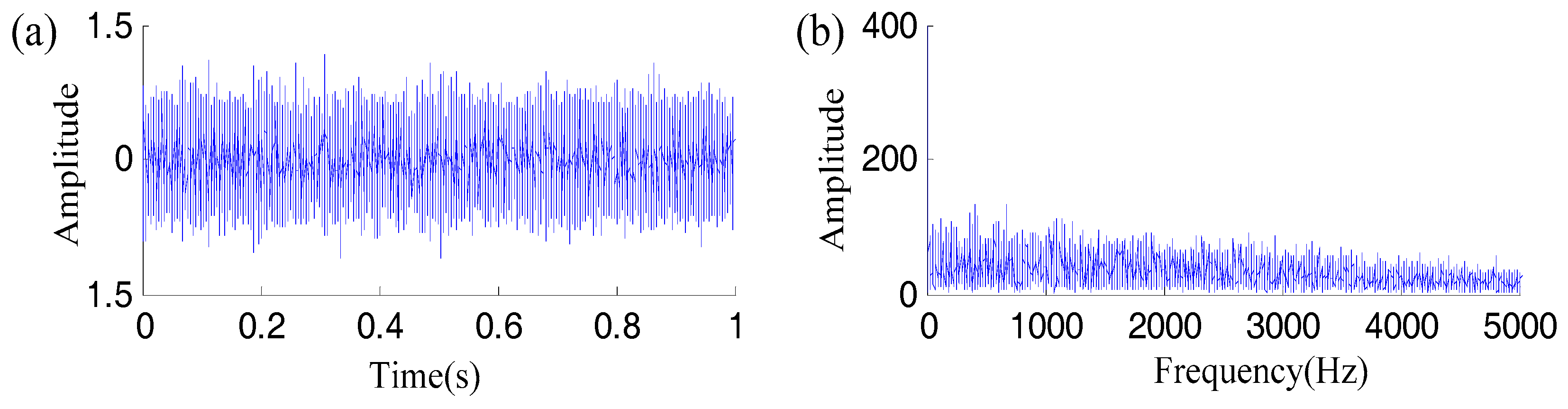
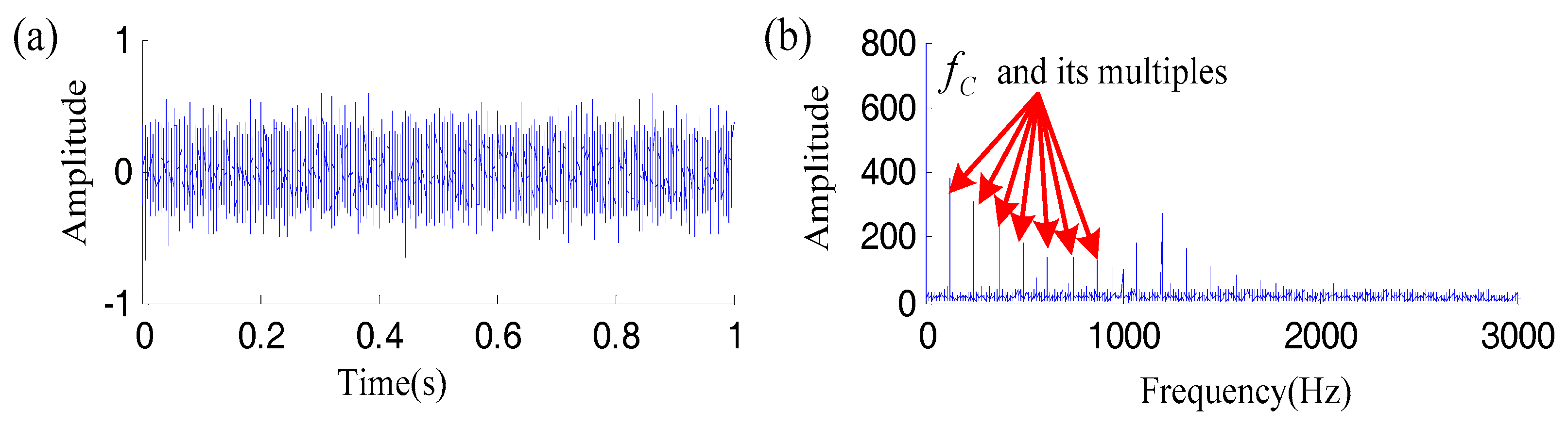
4. Simulation Studies

In order to verify the effectiveness of the MRSVD in the aspects of rolling bearing incipient fault detection, the mathematical model shown in Formula (8) was used to simulate the early fault vibration signal of a rolling bearing
x ( t ) = s ( t ) + n ( t ) + h ( t ) = m = M M A m e β ( t m T p i = M m τ i ) sin ( ω r ( t m T p i = M M τ i ) ) u ( t m T p i = M m τ i ) + n ( t ) + h ( t )
where n(t) is the noise signal added by the MATLAB function awgn.m,the signal-to-noise ratio (SNR) is set to −6, and h(t) is the harmonic interference signal that contains N harmonic signals, which can be expressed as h ( t ) = j = 1 N B j sin ( 2 π f i t ) , i.e., using the amplitude and the frequency of the jth harmonic signal, which are Bj and fj, respectively. The periodic shock signal caused by the fault contains 2M+1 impulses. In Formula (8), Am is the amplitude of the mth shock, β is the decay coefficient caused by the structural damping, Tp is the time period corresponding to the fault characteristic frequency, i.e., the fault feature frequency, fc = 1/Tp. u(t) is the unit impulse function, ωr is the excited frequency, and τi is the random variable whose mean value is zero and whose variance is between (0.01Tp, 0.02Tp), which is the effect of the random slippage of the rollers.
The parameters of the simulated signal are displayed in Table 1. The noise was directly added to the simulated periodic impulse signal before the harmonic interference signals were added. Therefore, the signal-to-noise ratio (SNR) in Table 1 is relative to the simulated periodic signal. The simulation signal was sampled at 20,000 samples s−1, and the number of sampling points was set to 20,000. After sampling, the simulated signal, along with the noise, the harmonic interference signals, and their Hilbert demodulation spectrums, are plotted in Figure 3. Due to the influences of the noise and the harmonic interference, it is impossible to judge the fault of rolling bearing from Figure 3a. In Figure 3b, the frequency differences of the harmonic components contained in the harmonic signal are mistakenly identified as the demodulation frequencies. However, the actual fault characteristic frequencies are not highlighted in Figure 3b.
The 2-row Hankerl matrixes were constructed for the simulation signal and their periodic impact, noise, and resonance components are denoted as H, Hs, Hn, and Hh, respectively. The result singular values of the SVD of the matrix H, Hs, Hn, and Hh are displayed in Table 2. The numerical results shown in Table 2 are consistent with the singular value analysis of the three kinds of signals (the periodic shock signal, the noise signal, and the harmonic signal) in Section 3.1 of this manuscript. To be specific, the two singular values obtained by the decomposition of the harmonic signals are quite different from each other, the two singular values obtained by the decomposition of noise signals are nearly equal, and the singular values obtained by the decomposition of periodic shock waves are different. However, the difference between them is neither too large nor close to zero.
The simulated signal shown in Figure 3 was decomposed using the MRSVD method, and the number of decomposed layers was set to 15. The singular values and the kurtosis coefficients corresponding to the obtained detail signals of each layer are shown in Figure 4a,b.
It can be seen from Figure 4a that the singular values of the first several detail signals decreased rapidly because the noise was removed relatively quickly at the beginning. Then the singular values of the detail signals decreased gradually with the increase of the number of layers. To be specific, the noise removal became slow with the increase of the number of decomposed layers.
As shown in Figure 4b, because the first detail signal contained a large amount of noise, its kurtosis coefficient was nearly equal to 3. As the number of decomposed layers increased, the kurtosis value also increased, because the noise component contained in the detail signal decreased layer by layer and the periodic impact component increased layer by layer. When the number of decomposed layers was 5, the kurtosis value of the detail signal reached a maximum, and the kurtosis value decreased with the increase of the decomposed layer because the periodic shock component contained in the residual approximate signal decreased layer by layer. Therefore, the conclusions pertaining to the kurtosis value analysis of the detail signals in Section 3.1 are verified in Figure 4b.
Figure 5 shows the time domain and frequency domain waveforms of the first detail signal obtained by the decomposition of the simulated signal via the MRSVD method. The main component of the signal in Figure 5 is the noise signal. Therefore, there is no highlighted frequency in the frequency spectrum of Figure 5. The time-domain and frequency-domain waveforms of the last layer of the approximate signal obtained by the decomposition of the simulated signal via the MRSVD method are plotted in Figure 6a,b. As stated in Section 3.1, most of the energy of the harmonic signal was retained in the last layer of the approximation signal, so the highlighted frequencies in Figure 6b are the harmonic frequencies f1, f2 and f3.
The five signals with maximum kurtosis were selected (see the red box in Figure 4b), and these five signals were added together in order to form a synthetic signal. Figure 7 shows the time-domain waveform of the synthetic signal and its Hilbert envelope demodulation spectrum. Although some noise was also contained in the synthetic signal, the fault characteristic frequency and its multiples are highlighted in the Hilbert envelope demodulation spectrum shown in Figure 7b.
In the above simulation analysis, the number of decomposed layers of the MRSVD method was set to 15 (Figure 4b). The corresponding sequence number of the detail signal with the maximum kurtosis value is 5. Therefore, when combined with the description of the decomposition layer number settings in Section 3.2, the number of decomposed layers of the MRSVD method only needed to be set to 10.

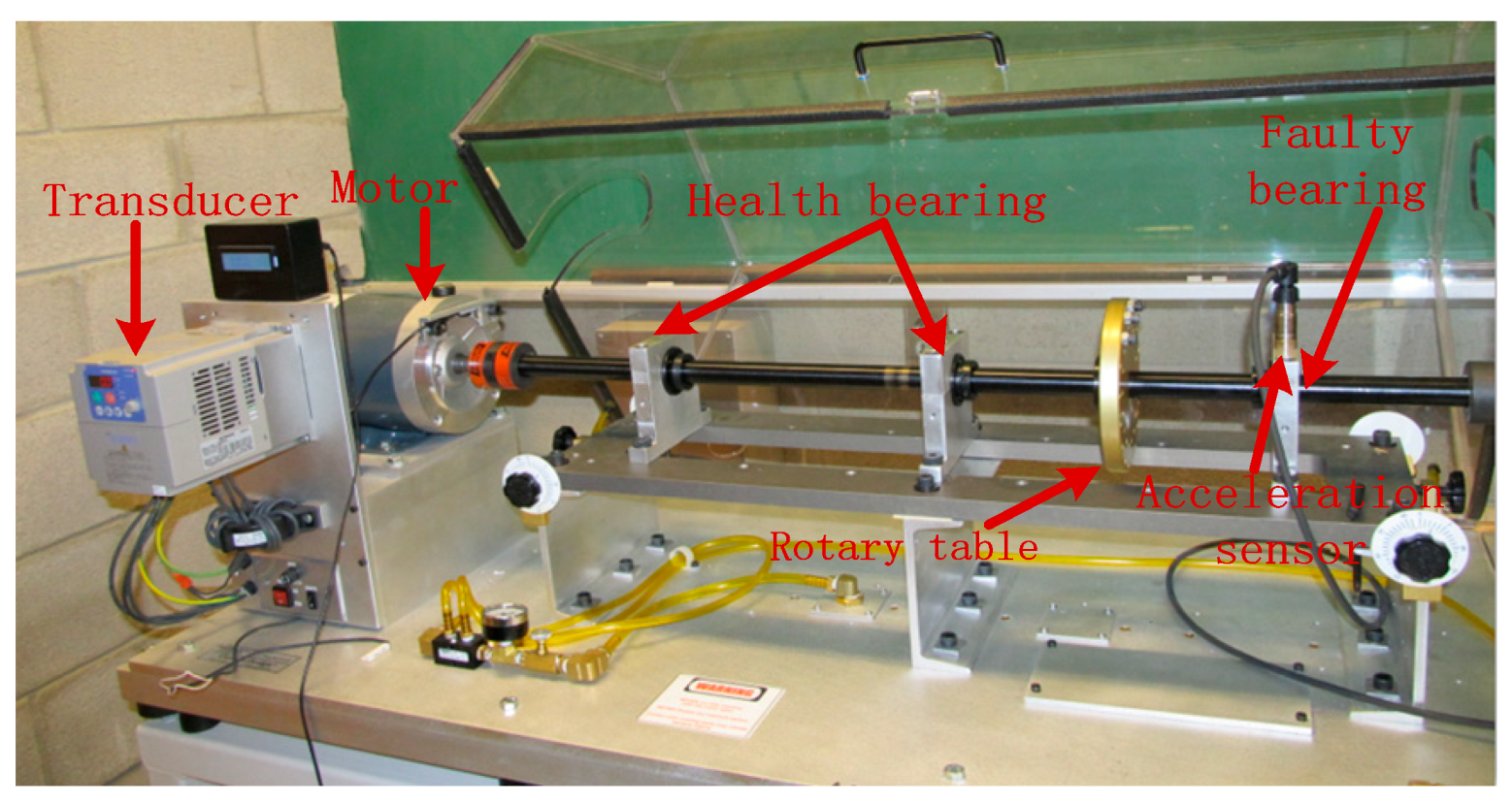
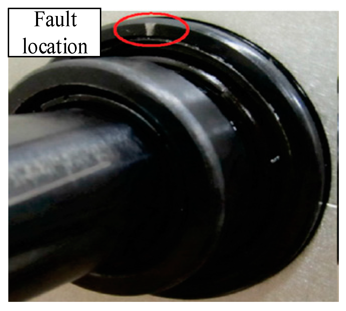
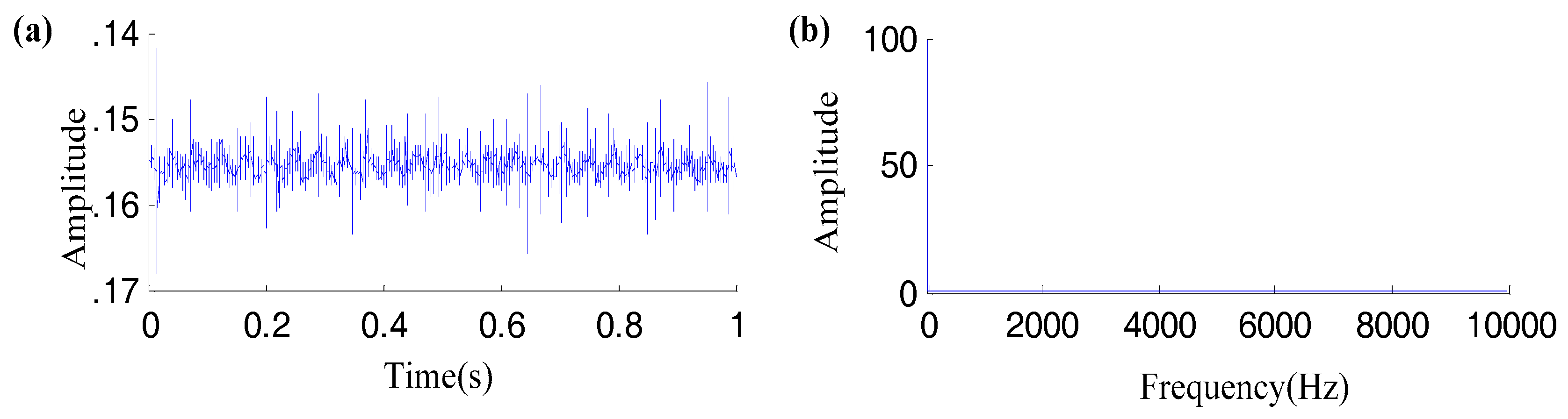
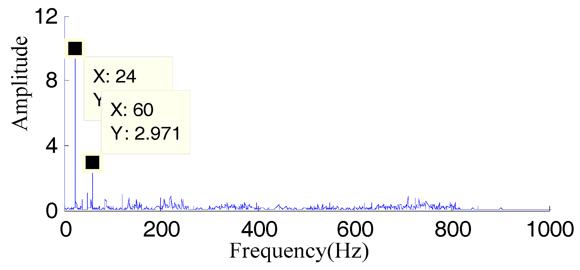
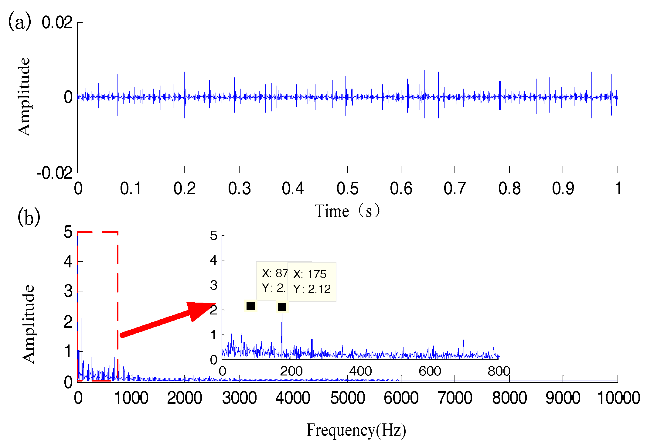
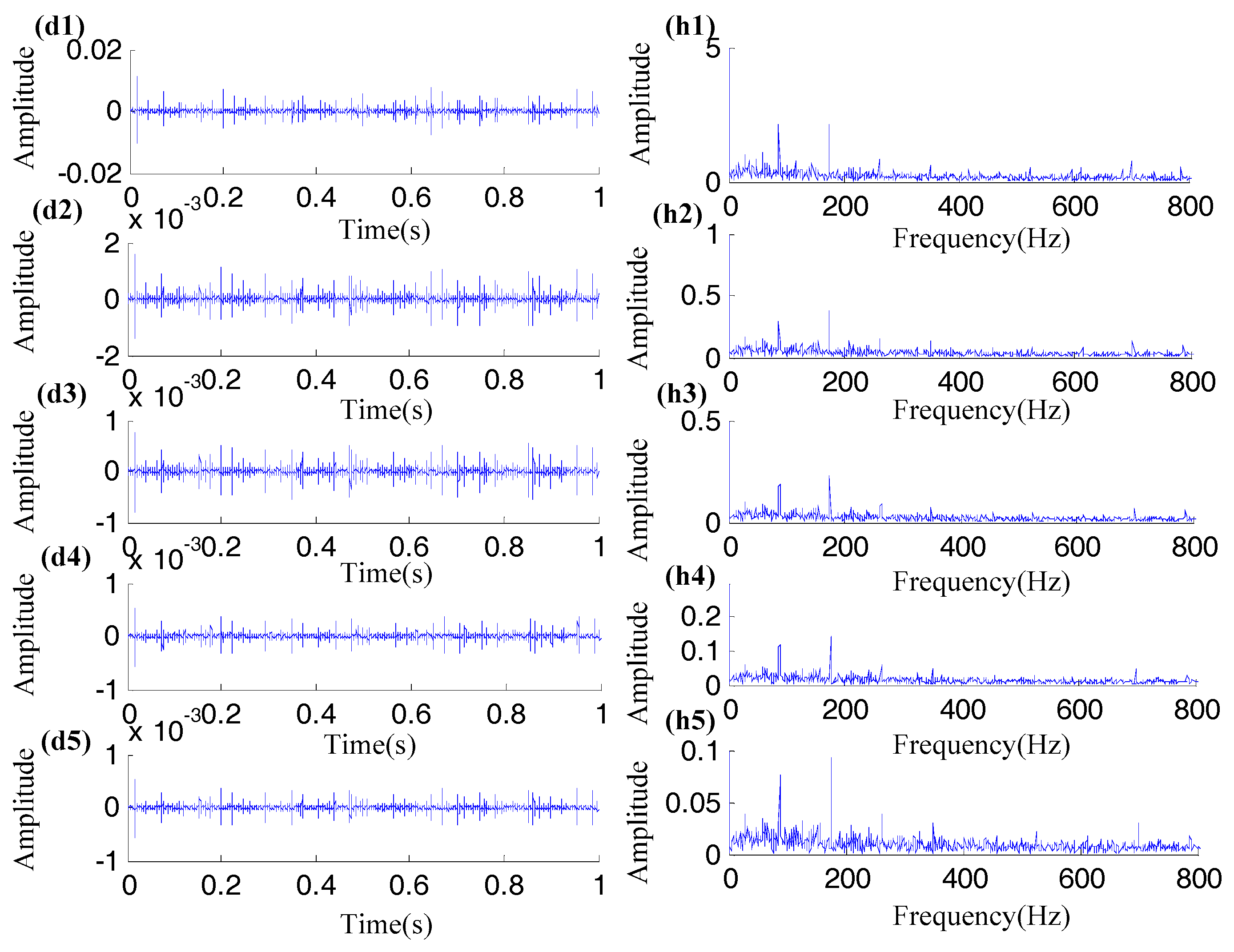
5. Experiment Studies

In order to verify the effectiveness of the MRSVD method in practical application, vibration signals of the outer race fault rolling bearing were collected from the experimental setup shown in Figure 8. The signal from the sensor (ICPR accelerometer, model 623C01) is fed to an NI data acquisition module (NI USB-6212 BNC) and is recorded by the computer with the LABVIEW software. The sampling frequency is 20 kHz and acquired data length is 40 k. The fault characteristics of incipient failure are not obvious; the periodic shock vibration associated with faults is often drowned in the background noise and the harmonic interference. Therefore, a more challenging condition is created at the experiment; the sensor signal conditioner is removed. Hence, the raw signal from sensor is not altered and not amplified. Obviously, the signal collected in this way is less clean and is considered more realistic. In the raw data, the interference, such as the power line frequency around 60 Hz, cannot be ignored. The background noise will be more obvious. For example, the noise caused by casualization error of the NI data acquisition module is inevitable and becomes relatively stronger when the raw signal voltage of the accelerometer output is very low.
The ER16K ball bearings, manufactured by Rexnord Industries, are used throughout the experiments. The bearing parameters are shown in Table 3. The outer race fault is in the top position, see Figure 9. In Table 3, the Ball Pass Frequency Outer Race (BPFO) and fr terms represent the characteristic frequency of outer race failure and the rotation frequency of the rotating shaft, respectively. To be specific, the frequency of the rotary shaft rotation frequency fr is the resonance harmonic signal caused by the imbalance of the rotary table.
The ER16K ball bearings, manufactured by Rexnord Industries, are used throughout the experiments. The bearing parameters are shown in Table 3. The outer race fault is in the top position, see Figure 9. In Table 3, the BPFO and fr terms represent the characteristic frequency of outer race failure and the rotation frequency of the rotating shaft, respectively. To be specific, the frequency of the rotary shaft rotation frequency fr is the resonance harmonic signal caused by the imbalance of the rotary table.
The rotation speed of the rotation axis was 1440 rpm, so fr = 12 Hz and BPFO = 85.728 Hz. The time domain waveform and the Hilbert envelope demodulation spectrum of the collected vibration signal with the noise and the resonance interference are shown in Figure 10a,b. For Figure 10b, the display interval of the coordinate axis is reduced, and a detailed graph is obtained in order to see the details shown in Figure 11. The resonant frequency of 24 Hz and the power line frequency of 60 Hz can be clearly seen in Figure 11. However, the failure characteristic frequency of the bearing outer race cannot be seen.
The measured signal shown in Figure 10a is decomposed by MRSVD. The time domain waveform and the Hilbert envelope demodulation spectrum of the detail signal with the maximum kurtosis value are displayed in Figure 12a,b. The periodic shock oscillations with single-sided attenuations which were caused by the bearing failure can be seen in Figure 12a. The characteristic frequency of the outer race failure (BPFO) and its double are highlighted in Figure 12b.
The five detail signals with maximum kurtosis values obtained using MRSVD decomposition are plotted in Figure 13d1–d5. Furthermore, their corresponding Hilbert envelope demodulation spectrums are shown in Figure 13h1–h5. In Figure 13h1–h5, in order to display the fault feature frequency more clearly, the display scope in the frequency domain is limited to the range of 0 Hz to 800 Hz. The time domain waveform and the Hilbert envelope demodulation spectrum of the detail signal with the maximum kurtosis value are also displayed in Figure 13d1,h1 in order to provide a comparison with the rest of the figures in Figure 13. Similarly to Figure 11, the periodic shock oscillations with single-sided attenuations caused by the bearing failure can also be seen in Figure 13d1–d5. The characteristic frequency of the outer race failure (BPFO) and its double are also highlighted in Figure 13h2–h5. Therefore, it can be determined that outer race fault exists in the roll bearing.

6. Conclusions

In this study, a new technique based on MRSVD has been developed for the initial fault detection of a rolling bearing. With this method, the raw bearing vibration signal acquired at the incipient failure stage, which contains the background noise, the harmonic interference, and the periodic impulse characteristics, can be decomposed to a series of approximate signals and detailed signals with different resolutions. Thus, the background noise, the harmonic interference, and the periodic impulse characteristics will correspond to different signal components. Theoretical and experimental analyses show that the first detail signal is mainly composed of noise and the last approximate signal is mainly composed of harmonic interference. Therefore, the periodic impulse characteristics that are related to the rolling bearing failure can be extracted from the detail signals (in addition to the first detail signal).
The advantages of the introduced approach include the following: (a) in contrast to the resonant demodulation approaches, this approach extracts the periodic impulse characteristics for demodulation analysis in order to identify the fault without relying on prior knowledge of the fault-excited resonance frequency; (2) this approach is computationally efficient, as except for the singular value decomposition of a two-row matrix, the algorithm only involves addition and subtraction.

Author Contributions

The topic of this research is designed by J.L. and S.Z.; Formal analysis is completed by J.L.; The first version of manuscript is prepared by J.L.; and this version of the manuscript is read, approved and substantially contributed by all authors.

Funding

This work was supported by the Natural Science Foundation of China (grant no. 51605405, 51975121, 51605406), the Science and Technology Innovation Project of Fujian Province, China (grant no. 2016H2003), the Natural Science Foundation of Fujian Province (grant no. 2018J01531), and the program for Innovative Research Team in Science and Technology at the Fujian Province University. Their support is gratefully acknowledged.

Acknowledgments

The authors wish to thank Y Wang and Y Zhang for their experimental work carried out at the University of Ottawa lab. They also wish to thank the Board member and the reviewer for their valuable suggestions and comments that have helped improve this paper.

Conflicts of Interest

The authors declare no conflict of interest.

References

  1. Randall, R.B.; Antoni, J. Rolling element bearing diagnostics-A tutorial. Mech. Syst. Signal Process. 2011, 25, 485–520. [Google Scholar] [CrossRef]
  2. Jaskaran, S.; Ashish, D.; Satinder, P.S. Rolling element bearing fault detection based on Over-Complete rational dilation wavelet transform and auto-correlation of analytic energy operator. Mech. Syst. Signal Process. 2018, 100, 662–693. [Google Scholar]
  3. Yaqub, M.F.; Gondal, I.; Kamruzzaman, J. Inchoate Fault Detection Framework: Adaptive Selection of Wavelet Nodes and Cumulant Orders. IEEE Trans. Instrum. Meas. 2012, 61, 685–695. [Google Scholar] [CrossRef]
  4. Zhang, W.; Peng, G.; Li, C. Rolling element bearings fault intelligent detection based on convolutional neural networks using raw sensing signal. In Advances in Intelligent Information Hiding and Multimedia Signal Processing; Springer International Publishing: Cham, Germany, 2017. [Google Scholar]
  5. Jiang, X.; Li, S.; Cheng, C. A novel method for adaptive multiresonance bands detection based on VMD and using MTEO to enhance rolling element bearing fault detection. Shock Vib. 2016, 2016, 7–20. [Google Scholar] [CrossRef]
  6. Cui, L.; Huang, J.; Zhang, F. Quantitative and localization detection of a defective ball bearing based on Vertical-Horizontal synchronization signal analysis. IEEE Trans. Ind. Electron. 2017, 64, 8695–8705. [Google Scholar] [CrossRef]
  7. Zhang, S.; Sun, Z.; Wang, M.; Long, J.; Bai, Y.; Li, C. Deep Fuzzy Echo State Networks for Machinery Fault Diagnosis. IEEE Trans. Fuzzy Syst. 2019. [Google Scholar] [CrossRef]
  8. Zhang, S.; Sun, Z.; Li, C.; Cabrera, D.; Long, J.; Bai, Y. Deep hybrid state network with feature reinforcement for intelligent fault diagnosis of delta 3D printers. IEEE Trans. Ind. Inform. 2019. [Google Scholar] [CrossRef]
  9. Wang, Y.; He, Z.; Zi, Y. A comparative study on the local mean decomposition and empirical mode decomposition and their applications to rotating machinery health detection. J. Vib. Acoust. 2010, 132, 613–624. [Google Scholar] [CrossRef]
  10. Yan, R.; Gao, R.X.; Chen, X. Wavelets for fault detection of rotary machines: A review with applications. Signal Process. 2014, 96, 1–15. [Google Scholar] [CrossRef]
  11. Wang, H.; Chen, J.; Dong, G. Feature extraction of rolling bearing’s early weak fault based on EEMD and tunable Q-factor wavelet transform. Mech. Syst. Signal Process. 2014, 48, 103–119. [Google Scholar] [CrossRef]
  12. Deng, L.; Zhao, R. Fault feature extraction of a rotor system based on local mean decomposition and Teager energy kurtosis. J. Mech. Sci. Technol. 2014, 28, 1161–1169. [Google Scholar] [CrossRef]
  13. Wang, S.; Chen, X.; Tong, C.; Zhao, Z. Matching synchrosqueezing wavelet transform and application to aeroengine vibration monitoring. IEEE Trans. Instrum. Meas. 2017, 66, 360–372. [Google Scholar] [CrossRef]
  14. Li, C.; Liang, M. Time-frequency signal analysis for gearbox fault detection using a generalized synchrosqueezing transform. Mech. Syst. Signal Process. 2012, 26, 205–217. [Google Scholar] [CrossRef]
  15. Osman, S.; Wang, W. A leakage-free resonance sparse decomposition technique for bearing fault detection in gearboxes. Meas. Sci. Technol. 2018, 29, 035004. [Google Scholar] [CrossRef]
  16. Cui, L.; Gong, X.; Zhang, J.; Wang, H. Double-dictionary matching pursuit for fault extent evaluation of rolling bearing based on the Lempel-Ziv complexity. J. Sound Vib. 2016, 385, 372–388. [Google Scholar] [CrossRef]
  17. Ding, X.; He, Q. Time-frequency manifold sparse reconstruction: A novel method for bearing fault feature extraction. Mech. Syst. Signal Process. 2016, 80, 392–413. [Google Scholar] [CrossRef]
  18. Zhang, S.; Sun, Z.; Long, J.; Li, C.; Bai, Y. Dynamic condition monitoring for 3D printers by using error fusion of multiple sparse auto-encoders. Comput. Ind. 2019, 105, 164–176. [Google Scholar] [CrossRef]
  19. Wang, Y.; Xiang, J.; Markert, R.; Liang, M. Spectral kurtosis for fault detection, diagnosis and prognostics of rotating machines: A review with applications. Mech. Syst. Signal Process. 2016, 66–67, 679–698. [Google Scholar] [CrossRef]
  20. Liang, M.; Bozchalooi, I.S. An energy operator approach to joint application of amplitude and frequency-demodulations for bearing fault detection. Mech. Syst. Signal Process. 2010, 24, 1473–1494. [Google Scholar] [CrossRef]
  21. Rodríguez, P.H.; Alonso, J.B.; Ferrer, M.A. Application of the Teager-Kaiser energy operator in bearing fault detection. ISA Trans. 2013, 52, 278–284. [Google Scholar] [CrossRef]
  22. Wang, H.; Gao, G.G.; Zeng, X.W. Wind Turbine Gearbox Fault detection Based on Wavelet Theory and Hilbert Demodulation Spectrum. Appl. Mech. Mater. 2015, 703, 390–393. [Google Scholar] [CrossRef]
  23. Liu, X.; Bo, L.; Peng, C. Application of order cyclostationary demodulation to damage detection in a direct-driven wind turbine bearing. Meas. Sci. Technol. 2014, 25, 25004–25011. [Google Scholar] [CrossRef]
  24. Wang, C.; Jiang, D.P.; He, Z.C. Research on fault diagnoses of rolling bearing based on the energy operator demodulation approach. Adv. Mater. Res. 2012, 588–589, 134–140. [Google Scholar] [CrossRef]
  25. Zhou, Y.; Chen, J.; Dong, G.M.; Xiao, W.B.; Wang, Z.Y. Application of the horizontal slice of cyclic bispectrum in rolling element bearings detection. Mech. Syst. Signal Process. 2012, 26, 229–243. [Google Scholar] [CrossRef]
  26. Saidi, L.; Ali, J.B.; Fnaiech, F. Application of higher order spectral features and support vector machines for bearing faults classification. ISA Trans. 2015, 54, 193–206. [Google Scholar] [CrossRef]
  27. Yunusa-Kaltungo, A.; Sinha, J.K. A comparison of signal processing tools: Higher order spectra versus higher order coherences. J. Vib. Eng. Technol. 2015, 3, 461–472. [Google Scholar]
  28. Yang, D.M.; Stronach, A.F.; MacConnell, P.; Penman, J. Third-order spectral techniques for the detection of motor bearing condition using artificial neural networks. Mech. Syst. Signal Process. 2002, 16, 391–411. [Google Scholar] [CrossRef]
  29. Yunusa-Kaltungo, A.; Sinha, J.K.; Nembhard, A.D. Use of composite higher order spectra for faults detection of rotating machines with different foundation flexibilities. Measurement 2015, 70, 47–61. [Google Scholar] [CrossRef]
  30. Li, F.; Meng, G.; Ye, L.; Chen, P. Wavelet transform-based higher-order statistics for fault detection in rolling element bearings. J. Vib. Control 2008, 14, 1691–1709. [Google Scholar]
  31. Howard, I.M. Higher-order spectral techniques for machine vibration condition monitoring. Proc. Inst. Mech. Eng. Part G J. Aerosp. Eng. 1997, 211, 211–219. [Google Scholar] [CrossRef]
  32. Shao, R.; Li, J.; Hu, W.; Dong, F. Multi-fault clustering and detection of gear system mined by spectrum entropy clustering based on higher order cumulants. Rev. Sci. Instrum. 2013, 84, 025107. [Google Scholar] [CrossRef] [PubMed]
  33. Yunusa-Kaltungo, A.; Sinha, J.K. Sensitivity analysis of higher order coherent spectra in machine faults detection. Struct. Health Monit. 2016, 15, 555–567. [Google Scholar] [CrossRef]
  34. Sheen, Y.T. On the study of applying Morlet wavelet to the Hilbert transform for the envelope detection of bearing vibrations. Mech. Syst. Signal Process. 2009, 23, 1518–1527. [Google Scholar] [CrossRef]
  35. Han, G.D.; Wan, S.T.; Lv, Z.J.; Liu, R.H.; Wang, J.; Tang, G.J. The Analysis of Gearbox Fault detection Research Based on the EMD and Hilbert Envelope Demodulation. Adv. Mater. Res. 2014, 926–930, 1800–1805. [Google Scholar] [CrossRef]
  36. Luo, J.; Yu, D.; Liang, M. A kurtosis-guided adaptive demodulation technique for bearing fault detection based on tunable-Q wavelet transform. Meas. Sci. Technol. 2013, 24, 055009. [Google Scholar] [CrossRef]
  37. Chibani, A.; Chadli, M.; Ding, S.X.; Braiek, N.B. Design of robust fuzzy fault detection filter for polynomial fuzzy systems with new finite frequency specifications. Automatica 2018, 93, 42–54. [Google Scholar] [CrossRef]
  38. Chadli, M.; Davoodi, M.; Meskin, N. Distributed state estimation, fault detection and isolation filter design for heterogeneous multi-agent linear parameter-varying systems. IET Control Theory Appl. 2016, 11, 254–262. [Google Scholar] [CrossRef]
  39. Zhu, X.; Xia, Y.; Chai, S.; Shi, P. Fault detection for vehicle active suspension systems in finite-frequency domain. IET Control Theory Appl. 2019, 13, 387–394. [Google Scholar] [CrossRef]
  40. Li, L.; Chadli, M.; Ding, S.X.; Qiu, J.; Yang, Y. Diagnostic observer design for t–s fuzzy systems: Application to real-time-weighted fault-detection approach. IEEE Trans. Fuzzy Syst. 2017, 26, 805–816. [Google Scholar] [CrossRef]
  41. Tian, Y.; Ma, J.; Lu, C.; Wang, Z. Rolling bearing fault detection under variable conditions using LMD-SVD and extreme learning machine. Mech. Mach. Theory 2015, 90, 175–186. [Google Scholar] [CrossRef]
  42. Jiang, H.; Chen, J.; Dong, G.; Liu, T.; Chen, G. Study on Hankel matrix-based SVD and its application in rolling element bearing fault detection. Mech. Syst. Signal Process. 2015, 52–53, 338–359. [Google Scholar] [CrossRef]
  43. Shen, F.; Chen, C.; Yan, R.; Gao, R.X. Bearing fault detection based on SVD feature extraction and transfer learning classification. In Proceedings of the Prognostics and System Health Management Conference (PHM), Beijing, China, 21–23 October 2015. [Google Scholar]
  44. Liao, Z.; Song, L.; Chen, P.; Guan, Z.; Fang, Z.; Li, K. An Effective Singular Value Selection and Bearing Fault Signal Filtering detection Method Based on False Nearest Neighbors and Statistical Information Criteria. Sensors 2018, 18, 2235. [Google Scholar] [CrossRef] [PubMed]
  45. Qiao, Z.; Pan, Z. SVD principle analysis and fault detection for bearings based on the correlation coefficient. Meas. Sci. Technol. 2015, 26, 085014. [Google Scholar] [CrossRef]
  46. Zhao, X.; Ye, B.; Chen, T. Theory of multi-resolution singular value decomposition and its application to signal processing and fault detection. J. Mech. Eng. 2010, 46, 64–75. [Google Scholar] [CrossRef]
Figure 1. The multi-resolution singular value decomposition (MRSVD) process of a given signal.
Applsci 09 04465 g001
Figure 2. The specific row vector forms of the Haj and Hdj matrixes. (a) The specific row vector forms of the Haj matrixes. (b) The specific row vector forms of the Hdj matrixes.
Applsci 09 04465 g002
Figure 3. Simulated signal (with noise and interference) and its Hilbert demodulation spectrum. (a) The waveform of the simulted signal in the time-domain. (b) The Hilbert demodulation spectrum of the simulted signal.
Applsci 09 04465 g003
Figure 4. The singular values and kurtosis coefficients corresponding to the obtained detail signals of each layer. (a) The singular values corresponding to the obtained detail signals of each layer. (b) The kurtosis coefficients corresponding to the obtained detail signals of each layer.
Applsci 09 04465 g004
Figure 5. The time and frequency waveform of the first detail signal. (a) The waveform of the first detail signal in the time-domain. (b) The waveform of the first detail signal in the frequency-domain.
Applsci 09 04465 g005
Figure 6. The time and frequency waveform of the last layer approximation signal. (a) The waveform of the last layer approximation signal in the time-domain. (b) The waveform of the last layer approximation signal in the frequency-domain.
Applsci 09 04465 g006
Figure 7. Time and Hilbert envelope demodulation spectrum of the extracted periodic impulse signal. (a) The waveform of the extracted periodic impulse signal in the time-domain. (b) The Hilbert envelope demodulation spectrum of the extracted periodic impulse signal.
Applsci 09 04465 g007
Figure 8. The test rig.
Applsci 09 04465 g008
Figure 9. The fault bearing used in the experiment.
Applsci 09 04465 g009
Figure 10. Time domain waveform and Hilbert envelope demodulation spectrum of the collected vibration signal with noise and resonance interference. (a) The waveform of the collected vibration signal in the time-domain. (b) The Hilbert envelope demodulation spectrum of the collected vibration signal.
Applsci 09 04465 g010
Figure 11. Details of Figure 9b from zooming out of the display range.
Applsci 09 04465 g011
Figure 12. Time domain waveform and Hilbert envelope demodulation spectrum of the detail signal with the maximum kurtosis value. (a) The waveform of the detail signal with the maximum kurtosis value. (b) The Hilbert envelope demodulation spectrum of the detail signal with the maximum kurtosis value.
Applsci 09 04465 g012
Figure 13. Time domain waveform of the five detail signals with the maximum kurtosis value and their corresponding Hilbert envelope demodulation spectrum. (d1d5) The five detail signals with maximum kurtosis values obtained using MRSVD decomposition. (h1h5) The corresponding Hilbert envelope demodulation spectrums of the five detail signals in (d1d5).
Applsci 09 04465 g013
Table 1. Parameters of the simulated signal. Signal-to-noise ratio (SNR).
AmTPMβωrSNRB1f1B2f2B3F3
10.008s2501500 Hz2048 Hz–61.3560Hz1.4230 Hz1.5800 Hz
Table 2. Result singular values of the singular value decomposition SVD of matrix H, Hs, Hn, and Hh.
Hankerl MatrixHHsHnHh
σ
σa354.861744.598269.4838346.2494
σd73.326414.270566.818317.5887
Table 3. The related parameters of the outer fault bearing. Ball Pass Frequency Outer Race (BPFO).
TypeRoll diameterPitch diameterNumber of rollsBPFO
ER16K7.94 mm38.52 mm93.572 fr

