Abstract
A new trajectory planning approach on the basis of the quintic Pythagorean–Hodograph (PH) curve is presented and applied to Delta robot for implementing pick-and-place operation (PPO). To satisfy a prescribed geometrical constraint, which indicates the distance between the transition segment curve and right angle of PPO trajectory is no greater than a prescribed value, the quintic PH curve is used to produce a connection segment path for collision avoidance. The relationship between the PH curve and constraint is analyzed, based on which PH curve is calculated simply. Afterwards, the trajectory is planned in different phases with different motion laws, i.e. polynomial motion laws and PH curve parameter-dependent motion laws, to obtain a smooth performance both in Cartesian and joint space. The relationship between the PH curve and constraint is also used to improve the efficiency of calculation, and the trajectory symmetry is used to reduce calculation time by direct symmetric transformation. Thus, real-time performance is improved. The results of simulations and experiments indicate that the approach in this paper can provide smooth motion and meet the real-time requirement under the prescribed geometrical constraint.
1. Introduction
In the past three decades, the use of parallel manipulators [1,2,3] has been increased in industrial and academic fields [4,5,6], especially in the fields of product transportation and classification, motion simulators, multi-dimensional force sensors, micro-operation consoles, precision positioning devices, etc., for their relative features like superior rigidity, higher accuracy, lighter mechanical construction, resulting in a homogenous and symmetric force/torque distribution, easier inverse kinematic calculations [7,8,9]. In recent years, researchers are increasingly inclined to concentrate on three translational degree-of-freedom (DOF) parallel manipulator [10,11,12,13]. As we all know, the Delta parallel robots [14,15] have effective mechanical structures [16], which makes the solution of its forward kinematic simpler. Because of its good characteristics, the Delta robot is often applied for high-speed pick-and-place applications with light-weight objects [9,17]. Pick-and-place is considered as a commonly used action [18] in palletizing and sorting in which objects are collected in an orderly manner and then put in their corresponding locations [19], however, due to the geometrically complicated surroundings, planning the robot’s pick-and-place movement is often difficult. Moreover, the research on optimizing the trajectories of parallel robots is relatively less than that of serial robots. Some work scenarios have requirements on the pick-and-place operation (PPO) path to avoid collisions between the workpiece and surroundings. Therefore, the study of trajectory planning for a parallel Delta robot with prescribed geometrical constraint is more challenging problem.
The PPO path of the Delta robot often includes two vertical segments and one horizontal segment [19]. Because of the existence of the right angle between the vertical and horizontal direction, the Delta robot is prone to shock and vibration, which has a bad effect on the rapid PPO. So, substituting the right angle by smooth curves is commonly used in related references [20]. It has the following advantages: (1) the overall route of smooth curves are shorter than the right angles; (2) Since the smooth curves have limited extreme curvature, it can maintain a relatively stable performance throughout its entire range rather than having a shock in the case of the right angle [21]. The above two advantages can decrease the PPO’s motion period and produce smoother motion characteristics. However, the degree of curvature of the smooth curve is important, since too much rounding could result in interference with objects in the robot workspace. Therefore, the PPO path should be transitioned through the smooth curve which deviates from the apex of the right angle by no more than a prescribed geometrical constraint.
The strategy of replacing the right angle by a smooth curve needs to meet some conditions, such as real-time interpolation calculation, smooth changes of the velocity, and smooth curve should match the PPO path, etc. Pythagorean-Hodograph curve [22] is very suitable for the above situation. The total arc length of the Pythagorean-Hodograph curves can be expressed as a polynomial with parameters [23], which makes real-time interpolation possible [21]. In addition, the Pythagorean–Hodograph (PH) curve has other advantages, for example, the curve has finite extremum curvature [24,25]. Due to the special property of the PH curve, it is widely used in path planning [26,27], obstacle avoidance [28], continuum manipulators [29], highways and railways design [30,31], and many other fields [32]. Researchers proposed interpolation methods of a PH curve of degree nine, however, it puts more emphasis on geometric issues, and the calculation of real-time interpolators is rather complicated [33].
This paper proposes a trajectory planning method for Delta parallel robot. (1) By utilizing quintic PH curves, the prescribed geometrical constraint is satisfied in PPO. (2) The relationship between the PH curve and the prescribed geometrical constraint is analyzed, and used to calculate the PH curve. (3) By using different motion laws in different motion phases, the stability and smoothness of motion are improved. The relationship between the PH curve and constraint is also used to improve the efficiency of the method, and the trajectory symmetry is used to generate part of the trajectory directly through a symmetric operation. In this way, the real-time performance is improved. The proposed method can realize the real-time PPO of the robot, which is beneficial to improving the industrial production efficiency and affecting the global economy. The prescribed geometrical constraint in the proposed method helps to make full use of the robot’s workspace and avoid collisions. Pick-and-place is known as one of the key operations in manufacturing and modern industrial system and the proposed method is flexible and widely applicable, so the proposed method can not only be applied on Delta robots, but also can be applied to various engineering areas such as raped sorting, palletizing, grabbing, warehousing, packaging, circuit board testing, automatic production lines system of food, medicine, and electronic products.
The paper is organized as follows. Section 2 introduces the kinematics and dynamics of the Delta robot, which lays the foundation for the following sections. Section 3 presents a trajectory planning approach on the basis of the quintic Pythagorean–Hodograph curve with a prescribed geometrical constraint, including PPO path, trajectory planning. The results of simulation and experiment are presented in Section 4. Discussion and conclusions are given in Section 5 and Section 6 separately.
2. Delta Parallel Robot
The three-degree-of-freedom Delta robot is illustrated in Figure 1. The Delta robot consists of a static platform, a mobile platform, and three chains. The mobile platform is attached to the static platform by three symmetric chains, each of which includes a rotationally active proximal link and a spatial unactuated parallelogram composed of spherical joint and link. With this design, the movement can be delivered to the mobile platform through three chains.
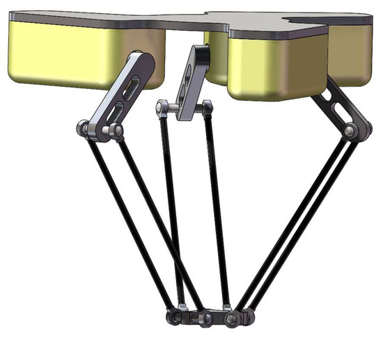
Figure 1.
Schematic of a Delta robot.
The kinematic analysis, including forward and inverse kinematics are introduced in reference [15].
The Delta robot dynamics is given as [4]
where M represents generalized inertia matrix, represents the joint coordinates , represents the Cartesian coordinates , and represent the set of active joint, the end effector (EE) location, the Lagrange multipliers vector and the input force vector, respectively, and represent gravitational vector and intrinsic parallel robot restriction vector respectively.
In PPO, the constraints on velocity, acceleration, torque, etc. are achieved through robot kinematics and dynamics [34].
3. Trajectory Planning
3.1. Path Planning
Delta robots are often applied to implement PPO in manufacture line. The PPO path is shown in Figure 2. From Figure 2, we can see PPO path includes vertical segments, which are and , and a horizontal segment, which is . In order to smooth the PPO path, curve transitions are adopted, that is, curve is used to replace the right angle formed by and , and curve is used to replace the right angle formed by and .
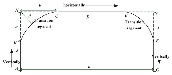
Figure 2.
Geometric path for pick-and-place operation (PPO).
Quintic PH curves, namely segments and , are used for the PPO path. In Figure 2, , , , , . The quintic PH curves in the PPO path illustrated in Figure 3 are given [35]
where
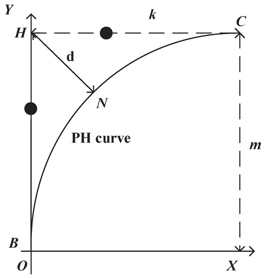
Figure 3.
The Pythagorean–Hodograph (PH) curve in the PPO path.
In the PPO path, for the purpose of simplifying the calculation and meeting the real-time requirements, assuming m equals k, thus the maximum deviation between the right angle and the PH curve can be obtained when , and see Proposition 1 for details. The parameter d in Figure 3 represents the maximum deviation between the right angle and the PH curve in the PPO path, which is called prescribed geometrical constraint. Therefore, we can get the quintic PH curve if d, the prescribed geometrical constraint, is given, and it is proved in the following proposition.
Proposition 1.
If , the maximum deviation between the right angle and the PH curve can be obtained when , on this basis, if d, the prescribed geometrical constraint, is given, the PH curve in the PPO path can be solved.
Proof.
, the curvature of PH curves, can be obtained by [24,30]
To ensure a connection between the horizontal and vertical segments, curvature must satisfy and . Then we can get the following equation
By substituting (6) into (5), the following equation can be obtained
The derivative of curvature can be calculated as
where . So,
When is less than 0.5, is positive, and when is greater than 0.5, is negative. Therefore, the curvature takes a maximum value at .
It can be obtained from the curvature calculation (7) that the curvature is symmetric with respect to . Point N in Figure 3 is the point when in PH curve is equal to 0.5, which means the coordinates of point N are the coordinates of . From the above derivation we can get the PH curve shown in Figure 3 is symmetrical about the line . Hence the maximum deviation between the right angle and PH curve can be obtained when . The coordinates of point N can be get by
The coordinates of point H are calculated by
Because m is equal to k, we can get the following equation.
So, d, the distance between point N and point H is as follows.
which is the maximum deviation between the right angle and PH curve.
Therefore, m can be determined once the required maximum deviation d between the right angle and PH curve is determined. As a result, the PH curve can be obtained according to (3). This completes the proof. □
Once d is determined, PH curve can be determined based on Proposition 1, then the workspace required for this PPO is determined, which is smaller than that in the PPO transitioned by right angle. It helps to make full use of the Delta robot’s workspace.
3.2. Trajectory Planning
A PPO motion in Figure 2 can be divided into the following phases.
- When EE moves along segment in the vertical direction, the EE’s velocity is specified as the polynomial motion law.where and , is the total time from point A to point B and is the current time in this segment. According to the boundary conditions, , we can get . From , we can get , where represents the velocity of point B, which acceleration is 0.
- When EE moves along the PH curve on segment , the velocity of end effector, which is dependent on the PH curve parameter , is as follows.From the above phase 1, we can get . Since the PPO trajectory is symmetrical, we can get . In order to ensure the acceleration’s continuity, the boundary prerequisites need to be satisfied. The velocity of point N, , can be seen as the minimum velocity, . So the coefficients can be calculated as follows: , , , , , . is the total time from point B to C, is current time in this segment. SoIn order to get at time , where is time interval, , can be calculated bywherewhereAccording to (17), we can get the following equation.Bringing Equations (16), (18), and (19) into (20), we can get the following formulawhere , . The fractions on the left of (21) can be factorized, then the following equation can be derived.where . Sowhere , , , .Hence can be obtained by solving the root of the following formulawhere .The function can be defined as,The derivative of the function is,where .Due to that and , the following formula holds. When , S takes the maximum value 0, as a result, , , and the molecule of the derivative is less than 0. When , has the maximum value , so , therefore, , as a result, . As , the denominator of the derivative is less than zero. That is, .Therefore, the function is monotonically increasing and has a unique solution. The Newton–Raphson iterations are used as follows, so as to meet the requirements of real-time calculation.Generally, the accuracy of the robot can be achieved in just 1 or 2 iterations.Hence the total time in this segment isThe EE’s coordinates can be obtained by converting the coordinates in the coordinate systems into robot base coordinate systems.
- When EE moves along segment in the horizontal direction, the velocity of end effector is specified as the polynomial motion law.where and , is the total time from point C to point D and is the current time in this segment. According to the boundary conditions, , we can get the following equation.From , we can get . Therefore, at the point D, the velocity is , and its acceleration is 0.
- When EE moves along segment in the horizontal direction, the velocity calculation method is similar to the method in phase 3.
- When EE moves along the PH curve in segment , the calculation method is similar to the method in phase 2.
- When EE moves along segment in the vertical direction, the velocity calculation method is similar to the method in phase 1.
4. Simulation and Experimental Results
4.1. Simulation and Analysis
The trajectory planning method proposed in this paper was simulated from the starting point coordinates (−152.5 mm, 0, −800 mm) to end point coordinates (152.5 mm, 0, −800 mm) using mm. Assume that the prescribed geometrical constraint was 6mm, m/s, m/s, m/s. As a comparison method, the trajectory planning based on motion superposition [35] was also simulated. In the comparison method, the maximum velocity in the vertical direction was set to 1.2 m/s, and the maximum velocity in the horizontal direction was set to 2.4 m/s, which were the same as the proposed method.
Figure 4 illustrates the path of the mentioned two approaches in base coordinate systems for Delta robot. The deviation between the right angle and PH curve in the proposed method is 6 mm, while the deviation in the comparison method is 3.7 mm. The deviation in the comparison method is fixed and cannot be changed, while the deviation in the proposed method can be set by specifying the prescribed geometrical constraint.
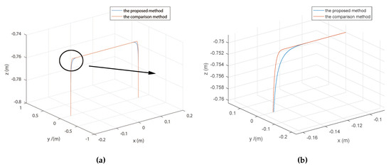
Figure 4.
The path of the two approaches. (a) The entire path, (b) the local path.
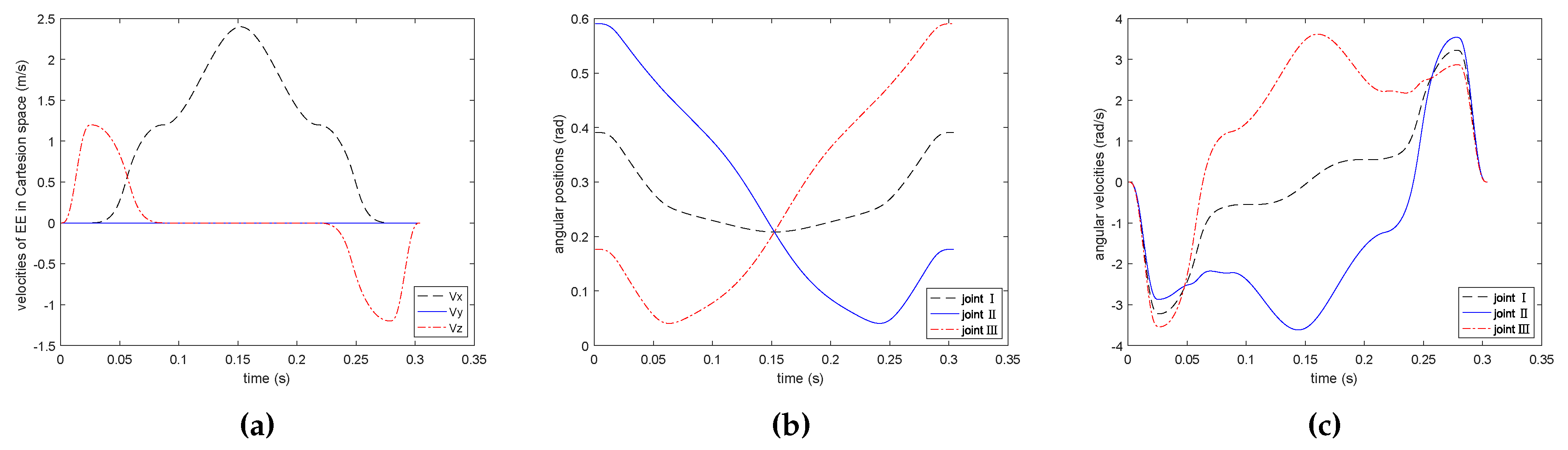
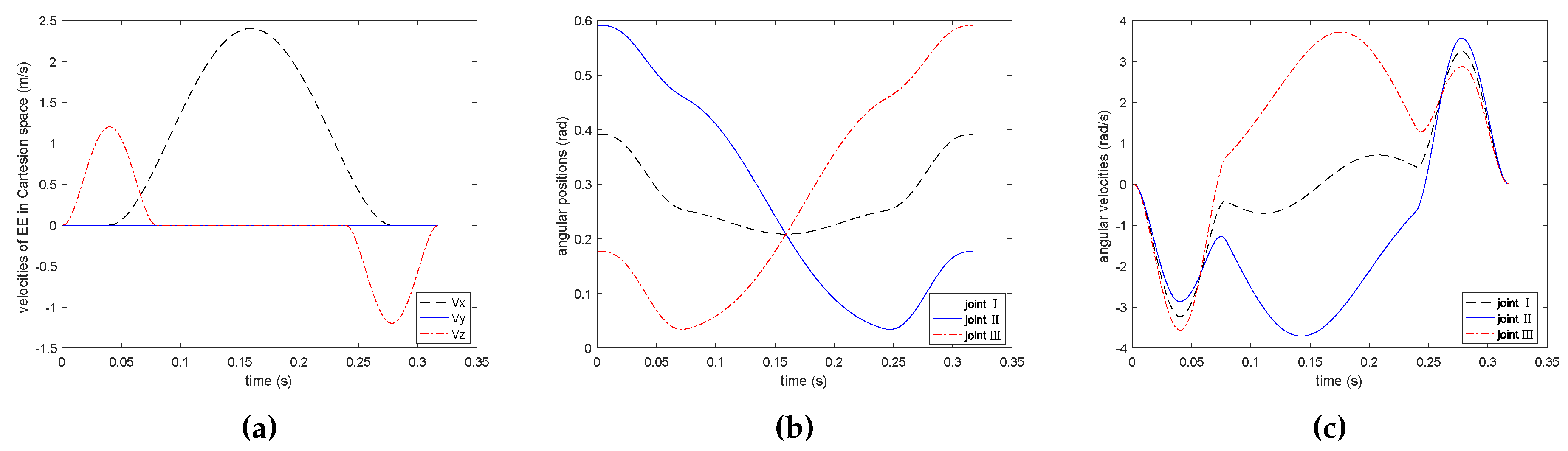
Figure 5 shows the EE’s velocities in Cartesian space, angular positions, and its velocities of PPO in joint space on the basis of the proposed method. Figure 6 shows the EE’s velocities in Cartesian space, angular positions, and its velocities of PPO in joint space on the basis of the comparison method. As illustrated in Figure 5 and Figure 6, the trajectory and the velocities of two methods in PPO are bounded and continuous in both Cartesian and joint space. What is more, the proposed method can also meet the prescribed geometrical constraint, which shows the proposed method is effective.
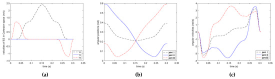
Figure 5.
Simulation results of trajectory planning with the proposed method. (a) end effector (EE)’s velocities in Cartesian space; (b) angular positions; (c) angular velocities.
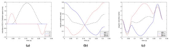
Figure 6.
Simulation results of trajectory planning with the comparison method. (a) EE’s velocities in Cartesian space; (b) Angular positions; (c) Angular velocities.
4.2. Experiment
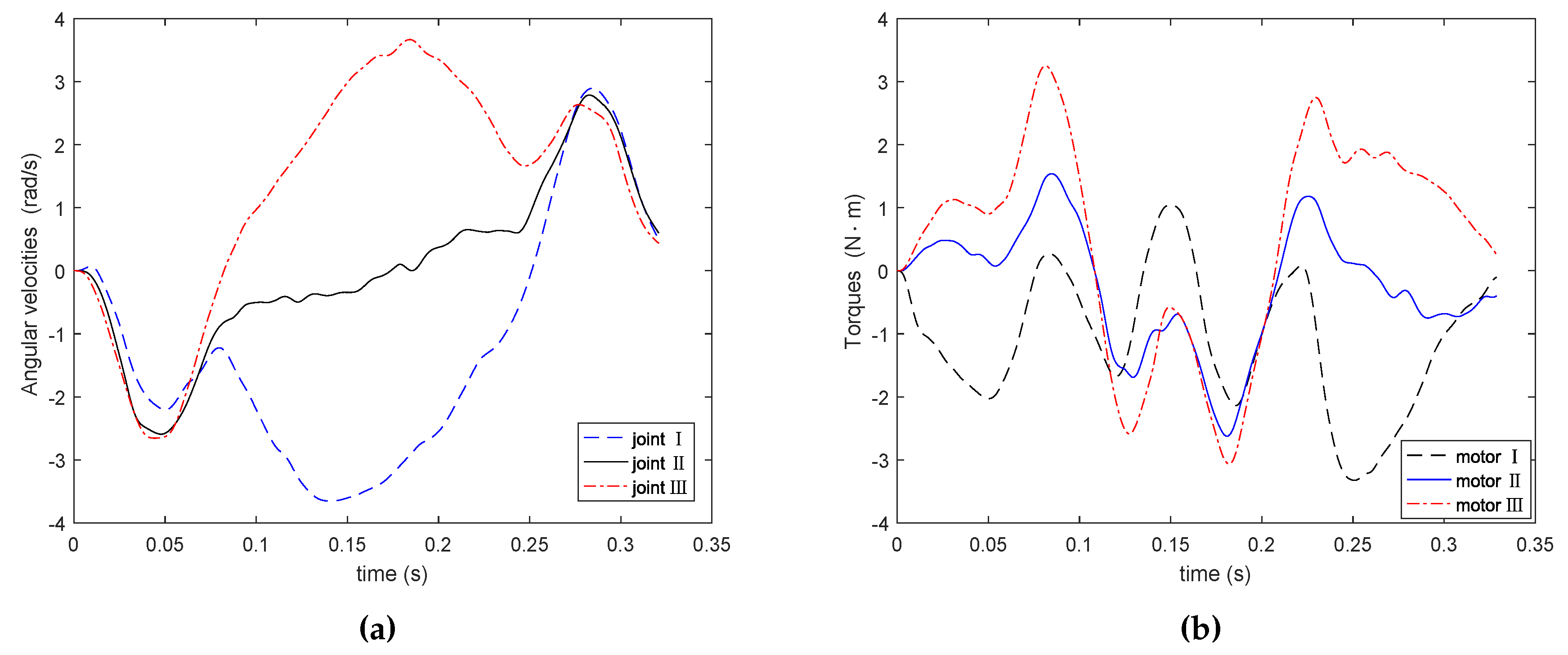
The experiment platform included PC, robotic controller, servo motion driver, Delta parallel mechanism, industrial camera and so on. Tests were implemented to verify the proposed method’s efficiency. The servo system used Panasonic’s MINAS A5-series servo motor and driver. The servo driver provided speed and torque monitor output signals, which could be collected by oscilloscope. Then the collected data was filtered. The starting point coordinates were (−152.5 mm, 0, −800 mm), and end point coordinates were (152.5 mm, 0, −800 mm), and mm. The prescribed geometrical constraint was 6 mm, m/s, m/s, m/s. The actuated joint’s angular velocity and the torques in motors of proposed method are shown in Figure 7. The actuated joint’s angular velocity and the torques in motors of comparison method are shown in Figure 8. In the experiments, once the prescribed geometrical constraint was given, the proposed method was immediately used to plan the trajectory. The controller ran on a PC with a 2130 MHz processor, and had a sampling interval 0.001 s. By optimizing the algorithms and programs, we implemented an iterative program with a single PPO with the average execution time of 0.207 ms, which satisfied the real-time requirements of the robot system.
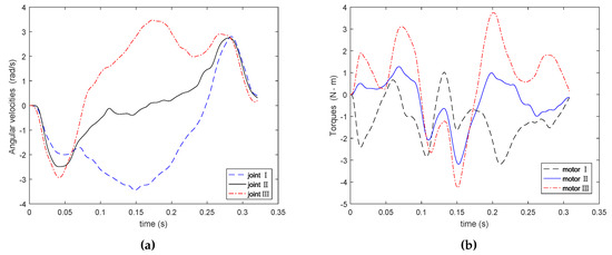
Figure 7.
Experimental results of angular velocity and torque by proposed method. (a) Angular velocity; (b) torque.
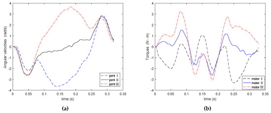
Figure 8.
Experimental results of angular velocity and torque by comparison method. (a) Angular velocity; (b) torque.
From the experimental results, we can get the conclusion that the experimental results match the simulation results well. Experiments also show that the proposed method can achieve the prescribed geometrical constraint and have good motion characteristics. As a result, the method proposed in this paper not only has good motion performance similar to the comparison method, but also can quickly plan the trajectory according to the prescribed geometrical constraint. Some techniques, such as symmetry, are used to achieve real-time operation of the system.
5. Discussion
The approach presented is beneficial to avoid collision between the Delta manipulator and the surroundings during PPO, so as to enhance the robot system’s safety. The results of simulations and experiments indicate both the proposed method and comparison method have good motion performance in PPO. Moreover, the proposed method also possesses the following benefits.
- The proposed method can be used to generate PPO trajectory of Delta parallel robot to meet a prescribed geometrical constraint, and can quickly and easily solve the relationship between PH curve and the prescribed geometrical constraint. The maximum deviation of the comparison method in reference [35] can be calculated bywhere , , , , , , , , is the angular between horizontal motion direction and X axis of robot base coordinate system, is the maximum speed in the vertical direction of PPO, is the maximum speed in the horizontal direction of the PPO, H, h and w are illustrated in Figure 2, t represents the current time. By bringing the root of the equation into (31), the maximum deviation can be obtained. Thus the maximum deviation in the comparison method is fixed and cannot be changed.It can be seen from the above process that the calculation of the deviation between the transition segment path and prescribed geometrical constraint in comparison method is more complicated. While the maximum deviation between the PH curve and right angle proposed in this paper is easier to be solved as shown in subsection—‘path planning’ of Section 3.
- In the subsection—‘trajectory planning’ of Section 3, there are some techniques to improve the computational efficiency, which helps to achieve real-time interpolation.
- (a)
- If there are two PPO trajectories that need to satisfy the same prescribed geometrical constraint, their PH curves in the coordinate system shown in Figure 3 are the same. Hence the PH curves do not have to be solved again, which saves time and is beneficial for improving system’s real-time performance.
- (b)
- Since both PPO trajectory and PH curve are symmetric, symmetry can be utilized to simplify the calculation to save time.
6. Conclusions
A trajectory planning approach on the basis of quintic Pythagorean–Hodograph curve for Delta robot with a prescribed geometrical constraint is proposed in this paper. Conventionally, trajectory planning methods of PPO present fixed deviation between the right angle and the actual transition curve. The proposed method uses the PH curves into the PPO path, so that the collision avoidance can be realized by the transition segment curve. By analyzing the relationship between the PH curve and constraint, we propose a brief algorithm to calculate the PH curve under the prescribed geometrical constraint. Then the trajectory is planned in different phases with different motion laws. The simulation and experiment results indicate the proposed method can provide smooth motion and meet the real-time requirement.
Author Contributions
Conceptualization, X.L.; methodology, X.L.; software, T.S.; validation, X.L. and T.S.; investigation, X.L. and T.S.; data curation, T.S.; writing—original draft preparation, X.L.; writing—review and editing, T.S.; funding acquisition, T.S.
Funding
This research was partially supported by the National Nature Science Foundation of China under Grant No. 51775002, the Nature Science Foundation of Beijing under Grant Nos. L172001, 3172009, L160001 and 3194047, and the Open Project Program of the State Key Laboratory of Management and Control for Complex Systems under Grant No. 20190101.
Conflicts of Interest
The authors declare no conflict of interest.
Acronyms
| PH | Pythagorean–Hodograph |
| PPO | Pick-and-place operation |
| DOF | Degree-of-freedom |
| EE | End effector |
References
- Joo, I.; Hong, J.; Yoo, S.; Kim, J.; Kim, H.S.; Seo, T.W. Parallel 2-DoF manipulator for wall-cleaning applications. Autom. Constr. 2019, 101, 209–217. [Google Scholar] [CrossRef]
- Tsai, L.W. Robot Analysis: The Mechanics of Serial and Parallel Manipulators; John Wiley and Sons: New York, NY, USA, 1999. [Google Scholar]
- Liu, X.J.; Han, G.; Xie, F.; Meng, Q. A novel acceleration capacity index based on motion/force transmissibility for high-speed parallel robots. Mech. Mach. Theory 2018, 126, 155–170. [Google Scholar] [CrossRef]
- Castañeda, L.A.C.; Juárez, A.L.; Chairez, I. Robust trajectory tracking of a Delta robot through adaptive active disturbance rejection control. IEEE Trans. Control Syst. Technol. 2015, 23, 1387–1398. [Google Scholar] [CrossRef]
- Li, C.S.; Gu, X.Y.; Xiao, X.; Lim, C.M.; Ren, H.L. A robotic system with multichannel flexible parallel manipulators for single port access surgery. IEEE Trans. Ind. Informat. 2019, 15, 1678–1687. [Google Scholar] [CrossRef]
- Cheng, H.; Yiu, Y.K.; Li, Z. Dynamics and control of redundantly actuated parallel manipulators. IEEE/ASME Trans. Mechatron. 2003, 8, 483–491. [Google Scholar] [CrossRef]
- Lin, C.J.; Chen, C.T. Reconfiguration for the maximum dynamic wrench capability of a parallel robot. Appl. Sci. 2016, 6, 80. [Google Scholar] [CrossRef]
- Lipiński, K. Modeling and control of a redundantly actuated variable mass 3RRR planar manipulator controlled by a model-based feedforward and a model-based proportional derivative feedforward feedback controller. Mechatronics 2016, 37, 42–53. [Google Scholar] [CrossRef]
- Brinker, J.; Corves, B.; Takeda, Y. Kinematic performance evaluation of high-speed Delta parallel robots based on motion/force transmission indices. Mech. Mach. Theory 2018, 125, 111–125. [Google Scholar] [CrossRef]
- Kosinska, A.; Galicki, M.; Kedzior, K. Design and optimization of parameters of Delta-4 parallel manipulator for a given workspace. J. Robot. Syst. 2003, 20, 539–548. [Google Scholar] [CrossRef]
- Affi, Z.; Romdhane, L.; Maalej, A. Dimensional synthesis of a 3-translational-DOF in-parallel manipulator for a desired workspace. Eur. J. Mech. A/Solids 2004, 23, 311–324. [Google Scholar] [CrossRef]
- Chablat, D.; Wenger, P. Architecture optimization of a 3-DOF translational parallel mechanism for machining applications, the orthoglide. IEEE Trans. Robot. Autom. 2003, 19, 403–410. [Google Scholar] [CrossRef]
- Kelaiaia, R.; Company, O.; Zaatri, A. Multiobjective optimization of a linear Delta parallel robot. Mech. Mach. Theory 2012, 50, 159–178. [Google Scholar] [CrossRef]
- Staicu, S.; Carp-Ciocardia, D.C. Dynamic analysis of Clavel’s Delta parallel robot. In Proceedings of the IEEE International Conference on Robotics and Automation, Taipei, Taiwan, 14–19 September 2003; pp. 4116–4121. [Google Scholar]
- Zhao, Y. Dimensional synthesis of a three translational degrees of freedom parallel robot while considering kinematic anisotropic property. Robot. Comput. Integr. Manuf. 2013, 29, 169–179. [Google Scholar] [CrossRef]
- Liu, X.J.; Wang, J.; Oh, K.K.; Kim, J. A new approach to the design of a DELTA robot with a desired workspace. J. Intell. Robot. Syst. 2004, 39, 209–225. [Google Scholar] [CrossRef]
- Mo, J.; Shao, Z.F.; Guan, L.; Xie, F.; Tang, X. Dynamic performance analysis of the X4 high-speed pick-and-place parallel robot. Robot. Comput.-Integr. Manuf. 2017, 46, 48–57. [Google Scholar] [CrossRef]
- Tsai, C.Y.; Wong, C.C.; Yu, C.J.; Liu, C.C.; Liu, T.Y. A hybrid switched reactive-based visual servo control of 5-DOF robot manipulators for pick-and-place tasks. IEEE Syst. J. 2015, 9, 119–130. [Google Scholar] [CrossRef]
- Boschetti, G.; Rosa, R.; Trevisani, A. Optimal robot positioning using task-dependent and direction-selective performance indexes: General definitions and application to a parallel robot. Robot. Comput. Integr. Manuf. 2013, 29, 431–443. [Google Scholar] [CrossRef]
- Huang, T.; Wang, P.F.; Mei, J.P.; Zhao, X.M.; Chetwynd, D.G. Time minimum trajectory planning of a 2-DOF translational parallel robot for pick-and-place operations. CIRP Ann. 2007, 56, 365–368. [Google Scholar] [CrossRef]
- Farouki, R.T.; Nittler, K.M. Efficient high-speed cornering motions based on continuously-variable feedrates. i. real-time interpolator algorithms. Int. J. Adv. Manuf. Technol. 2016, 87, 3557–3568. [Google Scholar] [CrossRef]
- Dong, B.H.; Farouki, R.T. Algorithm 952: PHquintic: A library of basic functions for the construction and analysis of planar quintic Pythagorean-hodograph curves. ACM Trans. Math. Softw. 2015, 41, 28. [Google Scholar] [CrossRef]
- Farouki, R.T. Construction of G2 rounded corners with Pythagorean-hodograph curves. Comput. Aided Geom. Des. 2014, 31, 127–139. [Google Scholar] [CrossRef]
- Farouki, R.T.; Neff, C.A. Hermite interpolation by Pythagorean hodograph quintics. Math. Comput. 1995, 64, 1589–1609. [Google Scholar] [CrossRef]
- Moon, H.P.; Farouki, R.T.; Choi, H.I. Construction and shape analysis of PH quintic Hermite interpolants. Comput. Aided Geom. Des. 2001, 18, 93–115. [Google Scholar] [CrossRef]
- Donatelli, M.; Giannelli, C.; Mugnaini, D.; Sestini, A. Curvature continuous path planning and path finding based on PH splines with tension. Comput. Aided Des. 2017, 88, 14–30. [Google Scholar] [CrossRef]
- Farouki, R.T.; Giannelli, C.; Mugnaini, D.; Sestini, A. Path planning with Pythagorean-hodograph curves for unmanned or autonomous vehicles. Part G J. Aerosp. Eng. 2018, 232, 1361–1372. [Google Scholar] [CrossRef]
- Giannelli, C.; Mugnaini, D.; Sestini, A. Path planning with obstacle avoidance by G1 PH quintic splines. Comput. Aided Des. 2016, 75, 47–60. [Google Scholar] [CrossRef]
- Singh, I.; Amara, Y.; Achille, M.; Pathak, P.M. Modeling of continuum manipulators using pythagorean hodograph curves. Soft Robot. 2018, 5, 425–442. [Google Scholar] [CrossRef]
- Walton, D.J.; Meek, D.S. G2 curve design with a pair of Pythagorean Hodograph quintic spiral segments. Comput. Aided Geom. Des. 2007, 24, 267–285. [Google Scholar] [CrossRef]
- Zheng, Z.; Wang, G.; Yang, P. On control polygons of Pythagorean hodograph septic curves. J. Comput. Appl. Math. 2016, 296, 212–227. [Google Scholar] [CrossRef]
- Walton, D.J.; Meek, D.S. Curve design with more general planar Pythagorean-hodograph quintic spiral segments. Comput. Aided Geom. Des. 2013, 30, 707–721. [Google Scholar] [CrossRef]
- Šír, Z.; Jüttler, B. Constructing acceleration continuous tool paths using pythagorean hodograph curves. Mech. Mach. Theory 2005, 40, 1258–1272. [Google Scholar] [CrossRef]
- Savsani, P.; Jhala, R.L.; Savsani, V.J. Comparative study of different metaheuristics for the trajectory planning of a robotic arm. IEEE Syst. J. 2016, 10, 697–708. [Google Scholar] [CrossRef]
- Su, T.T.; Cheng, L.; Wang, Y.K.; Liang, X.; Zheng, J.; Zhang, H.J. Time-optimal trajectory planning for Delta robot based on quintic Pythagorean-Hodograph curves. IEEE Access 2018, 6, 28530–28539. [Google Scholar] [CrossRef]

© 2019 by the authors. Licensee MDPI, Basel, Switzerland. This article is an open access article distributed under the terms and conditions of the Creative Commons Attribution (CC BY) license (http://creativecommons.org/licenses/by/4.0/).