Article

Amplitude Distribution of Partial Discharge Signals on Tunnel-Installed High-Voltage Cables

1
Department of Electrical Engineering, Shanghai Jiao Tong University, Shanghai 200240, China
2
State Grid Zhejiang Electric Power Research Institute, Hangzhou 310014, China
*
Author to whom correspondence should be addressed.
Appl. Sci. 2019, 9(21), 4595; https://doi.org/10.3390/app9214595
Submission received: 26 September 2019 / Revised: 18 October 2019 / Accepted: 23 October 2019 / Published: 29 October 2019
(This article belongs to the Section Electrical, Electronics and Communications Engineering)

Abstract

:
For 110 kV and above tunnel-installed high-voltage (HV) cross-linked poly-ethylene (XLPE) cable systems, it is a normal procedure to adopt a cross-bonding scheme. The high-frequency current method is frequently used in the cross-bonded cable systems for on-site or online partial discharge (PD) detection by monitoring the signals on the cross-bonding wires. To further study the amplitude distribution characteristics of the PD signals, a parametric characteristic admittance model of a three-phase cable system in a tunnel is established based on Tylavsky’s formulas. The model is used to calculate the amplitude distribution formula of the PD pulse current on the cross-bonding wires. In addition, the influence of cable laying and tunnel environment on the amplitude distribution is also studied. Finally, the correctness of the model and the conclusion are verified by simulation experiments and on-site tests. The results show that the signal amplitude distribution is determined by the ratio of the characteristic admittances. As the distance between the cables and the distance from the inner wall of the tunnel increase, the amplitude difference gradually decreases.

1. Introduction

Partial discharge (PD) is an important characterization of the insulation defects in cross-linked poly-ethylene (XLPE) cables [1,2,3]. Through on-site or online detection of PD signals, the state of the XLPE cables can be evaluated without power supply interruptions, which can help find the early degradation of the cable as soon as possible, thus improving the reliability of the power grid [4,5,6,7]. The high-frequency current method is commonly used in the PD detection of power cables. This method generally has a detection frequency band of 3–30 MHz [8]. For 110 kV and above HV XLPE cable systems, it is normal procedure to adopt a cross-bonding scheme, as shown in Figure 1. The high-frequency current transformers are installed on the cross-bonding connections of the cable metal sheaths through a non-contact method. These can detect the PD pulse current inside the cables without affecting the normal operation of the cable system [9,10].
As an increasing area of interest, the distribution of PD signals on the three-phase cross-bonding wires can be used as an important tool for PD location and eliminating the external disturbance [11,12,13]. However, previous studies are mainly based on fixed simulation parameters or a determined experimental environment, without considering the impact of cable laying parameters. In fact, the laying method and laying environment of HV cables have an inseparable relationship with the propagation of pulse current in the cable and will also affect the amplitude distribution of PD signals, which has not yet been seen in relevant research papers.
In order to discuss the distribution characteristics of the PD signals on the cross-bonding wires under different laying conditions, it is necessary to establish a cable system model for theoretical analysis. Existing cable modeling tools such as ATP (alternative transients program) are mostly based on Ametani’s distributed parameter model of directly buried cables [14,15]. This model uses Pollaczek’s formula [16] to calculate the earth return path impedance. However, Pollaczek’s formula is not suitable for the widely used tunnel-installed HV cable systems since it assumes that the conductors are completely surrounded by the earth. For underground tunnels, Tylavsky proposed a set of high-frequency formulas and low-frequency approximation formulas for calculating the earth return impedance [17]. Wu et al. [18] clarified its physical meaning and application scope by theoretical analysis and case calculation. Tylavsky’s formulas have a good accuracy at high frequencies by taking the proximity effect and skin effect into consideration. In [19], the low-frequency approximation formulas are used to study the propagation of traveling waves in the cross-bonded cable system, but it does not involve the current amplitude distribution and the influence of the laying parameters.
In this paper, a characteristic admittance model of three-phase cable systems is established based on Tylavsky’s formulas, and thus the formula of the amplitude distribution of PD pulse current on cross-bonding wires is obtained. On this basis, the influence of parameters such as tunnel radius, earth resistivity, cable center spacing, and the distance between the cable and the inner wall of the tunnel is studied. The model and conclusions is verified by experiments and on-site tests.

2. Cable Model

2.1. Distributed Parameters of Tunnel-Installed Cables

The three-phase cable can be regarded as a transmission line system consisting of 6 conductors. The propagation characteristics of the voltage and current on the conductors are determined by the distributed impedance matrix Z (unit: Ω) and the distributed admittance matrix Y (unit: S). The skin effect in the metal sheath is enhanced at high frequencies and the current is bound to the inner surface and outer surface of the sheath, which makes the transfer impedance decrease rapidly and it can be ignored [20]. In this case, the distributed parameter matrix Z and Y of the three-phase cable are as follows:
Z = [ z c c z m u z m u z s s z m u z m u z m u z c c z m u z m u z s s z m u z m u z m u z c c z m u z m u z s s z s s z m u z m u z s s z m u z m u z m u z s s z m u z m u z s s z m u z m u z m u z s s z m u z m u z s s ]
Y = [ y c s 0 0 y c s 0 0 0 y c s 0 0 y c s 0 0 0 y c s 0 0 y c s y c s 0 0 y s s y m u y m u 0 y c s 0 y m u y s s y m u 0 0 y c s y m u y m u y s s ]
where zcc, zss, zss, and zmu represent the self-impedance of the inner conductor, self-impedance of the metal sheath, and mutual impedance between the conductors, respectively. yss = yse + ycs + 2ymu, where ycs, yse, and ymu are the admittance of the inner conductor, admittance of the metal sheath to the earth, and mutual admittance between the metal sheaths, respectively. The formulas to calculate the impedance and admittance of directly buried cables have been given in [14,15]. The calculation of the admittance of tunnel-installed cables is the same, but the self-impedance zs and mutual impedance zm used to obtain the impedances zcc, zss zss, and zmu need to be calculated by Tylavsky’s high-frequency formulas.
Figure 2 shows the structure of the tunnel-installed cables, where R represents the radius of tunnel, b represents the distance from cable to the tunnel center, d represents the center spacing of the cables, θ represents the included angle between two cables, and r1, r2, and r3 represent the radius of the inner conductor, insulating layer, and metal sheath respectively. In this paper, the unit of all the length variables is meter and that of the angle is rad. Then the self-impedance zs and mutual impedance zm of the cable-ground loop are [18]:
z s = j ω μ 0 2 π ln R r + m ρ 2 π R K 0 ( m R ) K 1 ( m R ) + m ρ 2 π R n = 1 1 n [ b ( b + r ) R 2 ] n × [ m R μ e K n ( m R ) + n K n ( m R ) μ e n m R K n ( m R ) K n ( m R ) ]
z m = j ω μ 0 2 π ln R d + m ρ 2 π R K 0 ( m R ) K 1 ( m R ) + m ρ 2 π R n = 1 cos n θ n ( b 2 R 2 ) n × [ m R μ e K n ( m R ) + n K n ( m R ) μ e n m R K n ( m R ) K n ( m R ) ]
where ρ (unit: Ω∙m) and μe (no units) are the resistivity and the relative permeability of the earth respectively, ω (unit: rad/s) is the angular frequency, m = (jωμeμ0/ρ)1/2 and Kn represents the n-th order second modified Bessel function. To simplify the calculation, assume that the three cables are completely symmetrical, that is, the structure parameters of each cable are the same, and the distance and angle between any two cables are equal. In this case, d and b are represented by the geometric mean distance of the actual distance.

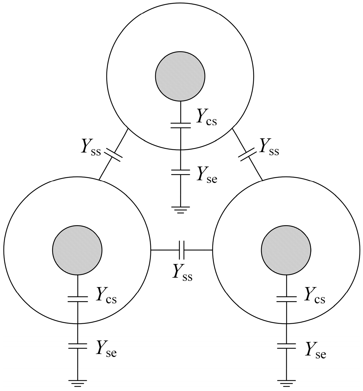
2.2. Cable Characteristic Admittance Model

The conductors are coupled to each other in a three-phase cable system, and therefore the voltage and current on each conductor is affected by the voltage and current on other conductors. The three-phase cable system can be transformed into a number of independent two-conductor transmission lines by using a modal transformation, then the characteristic admittance matrix Yc can be obtained from the distributed parameter matrix Z and Y [21]:
Y c = Z 1 T V λ T V 1
where λ is the propagation constant matrix of each mode after decoupling and TV is the voltage transformation matrix. λ and TV are the eigenvalues and eigenvector matrix derived from the diagonalization of the matrix product ZY, that is [21]:
T V 1 Z Y T V = λ 2
Similar to the two-conductor transmission line, the characteristic admittance matrix Yc characterizes the relationship between the voltage and the current on the multi-conductor transmission line. Based on the assumption that the cable is completely symmetrical, the extended matrix of the Clarke transform matrix can be used as the voltage transform matrix TV [20]. Equations (1), (2), and (6) are substituted into Equation (5) and simplified to obtain Yc:
Y c = [ Y c s 0 0 Y c s 0 0 0 Y c s 0 0 Y c s 0 0 0 Y c s 0 0 Y c s Y c s 0 0 Y s e + Y c s + 2 Y s s Y s s Y s s 0 Y c s 0 Y s s Y s e + Y c s + 2 Y s s Y s s 0 0 Y c s Y s s Y s s Y s e + Y c s + 2 Y s s ]
where:
Y c s = y c s z c c z s s
Y s e = y s s 2 y m u y c s 2 z m u + z s s
Y s s = 1 3 y s s + y m u y c s z s s z m u 1 3 y s s 2 y m u y c s 2 z m u + z s s
where Ycs is the coaxial characteristic admittance, namely, the reciprocal of the characteristic impedance of a single coaxial cable. Ycs is only related to the structure of the cable, usually between 0. 025 S and 0.1 S. Yse is the characteristic admittance between the cable sheath and the earth, and Yss is the characteristic admittance between the sheaths of the cable. Yse and Yss are affected by the external environment of the cable system. If Yc is regarded as a nodal admittance matrix, it can be expressed in the form of self-admittance and mutual admittance, as shown in Figure 3.
Figure 4 shows the frequency variation curves of the real parts of the characteristic admittances Ycs, Yse, and Yss. The laying parameters are shown in Table 1 and the relative permeability value is 1. The real parts of the characteristic admittances changed very slowly at high frequencies. At the same time, the imaginary parts are 1 to 4 orders of magnitude smaller than their real parts, and thus can be ignored [20]. Considering that the detection band of the high-frequency current method is usually between 3 to 30 MHz, the characteristic admittances Ycs, Yse and Yss can be regarded as fixed values in this range. In this paper, the admittances are calculated at 10 MHz.

3. Amplitude Distribution Characteristics of Signals on Cross-bonding Wires

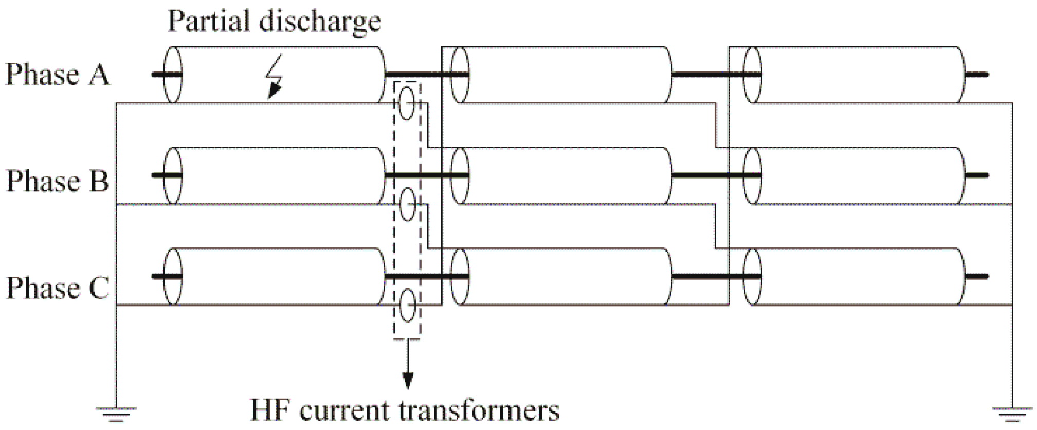
3.1. Current Reflection at Cross-Bonding Links

The characteristic admittance matrix Yc of a three-phase cable system changes after the cross-bonding link, causing current reflection. If the cross-bonded line length is ignored, the transmission coefficient Tbond is as follows [21]:
T bond = E + ( M Y c M T Y c ) ( M Y c M T + Y c ) 1
where E is a 6 × 6 identity matrix. M represents the rearrangement of the characteristic admittance matrix Yc after cross-bonding:
M = [ 1 0 0 0 0 0 0 1 0 0 0 0 0 0 1 0 0 0 0 0 0 0 1 0 0 0 0 0 0 1 0 0 0 1 0 0 ]
Equation (7) is then substituted into Equation (11) and the matrix form of the transmission coefficient Tbond is obtained:
T bond = [ 1 T c c T c c T s c 0 T s c T c c 1 T c c T s c T s c 0 T c c T c c 1 0 T s c T s c T c s T c s 0 1 T s s T s s 0 T c s T c s T s s 1 T s s T c s 0 T c s T s s T s s 1 ]
where,1
{ T c c = T s s = 1 3 + 4 α T c s = 2 + 2 α 3 + 4 α T s c = 2 3 + 4 α
α = 3 Y s s + Y s e Y c s
where Tcc, Tcs, Tss and Tsc are the reflection coefficients from inner conductor to inner conductor, from inner conductor to metal sheath, from metal sheath to inner conductor, and from metal sheath to metal sheath, respectively. According to the characteristic admittance model, Yss and Yse are the characteristic admittances between the cable and the external environment, while Ycs is the characteristic admittance inside the cable. Therefore, α can be regarded as the ratio of the external characteristic admittance to the internal characteristic admittance. From Equation (14), it can be seen that the reflection of the current at the cross-bonding is only related to the characteristic admittance ratio α.

3.2. Amplitude Distribution of PD Signal

PD usually occurs only in one phase of the three-phase cables. Pulse currents with the same amplitude and opposite polarity will be induced in the inner conductor and metal sheath of the cable [22]. The currents propagate in a coaxial mode, so the distribution of the current amplitude on each conductor is not affected by attenuation. Assuming that the PD is in phase A, the incident current at its adjacent cross-bonding joint is Iinc= [Ip 0 0 − Ip 0 0]T, where Ip represents the amplitude of the current when it propagates to the cross-bonding joint. The unit of the current variables is A. The current amplitude Icb at the cross-bonding joint is the product of the transmission coefficient Tbond and the incident current Iinc:
I cb = T bond I inc = I p 4 α + 3 [ 4 α + 1 1 1 2 α 1 1 2 α 1 ]
The 4th, 5th, and 6th elements in Icb are the currents of the cross-bonding wires in phase A, B, and C (the phase sequence is based on the phase of the discharge side, as shown in Figure 1). When the PD occurs inside the cable, the amplitude distributions of the signals on its adjacent cross-bonding wires have the following characteristics:
(1)
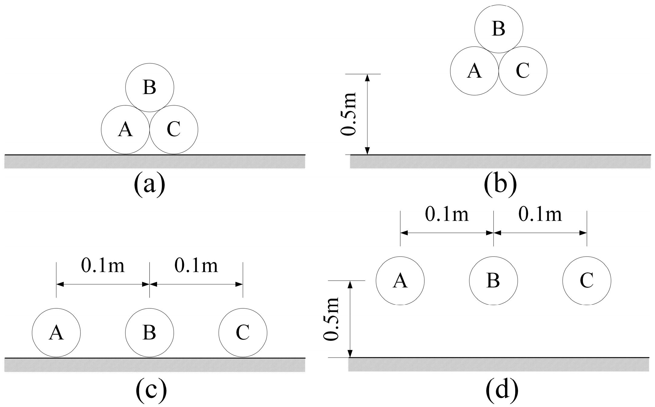
The current signals on the two cross-bonding wires connected to the defective phase are equal and denoted as Imajor. In the case of A-B, B-C, and C-A, as shown in Figure 1, if PD occurs in phase A, the signals on wire A and wire C are the same.
(2)
The current signal on the remaining cross-bonding wire is denoted as Iminor. The current Iminor has the same polarity with Imajor, but the amplitude is smaller. The proportional relationship between the two currents is determined by the characteristic admittance ratio α:
I m a j o r I m i n o r = 1 + 2 α
When the PD current signal passes through the first cross-bonding joint, it will no longer be composed of only the coaxial mode. It comprises the coaxial mode, the inters heath mode, and the earth mode [23]. The propagation velocity and attenuation rates of the three modes are different to each other, so a single pulse will gradually attenuate and be separated into multiple pulses as the propagation distance increases. Unlike the directly buried cables, the propagation velocity of the inters heath mode and the earth mode is often greater than or close to the propagation velocity of the coaxial mode for tunnel-installed cables, and thus cannot be neglected [19]. At the same time, the attenuation rate of the inters heath mode and the earth mode will vary significantly with frequency. Therefore, the amplitude distribution of the PD signal after passing through the first cross-bonding joint will become very complicated and may exhibit different distribution characteristics, which limits its guidance effect on on-site detection. For that reason, this paper focuses on the amplitude distribution at the adjacent joints to the PD source.

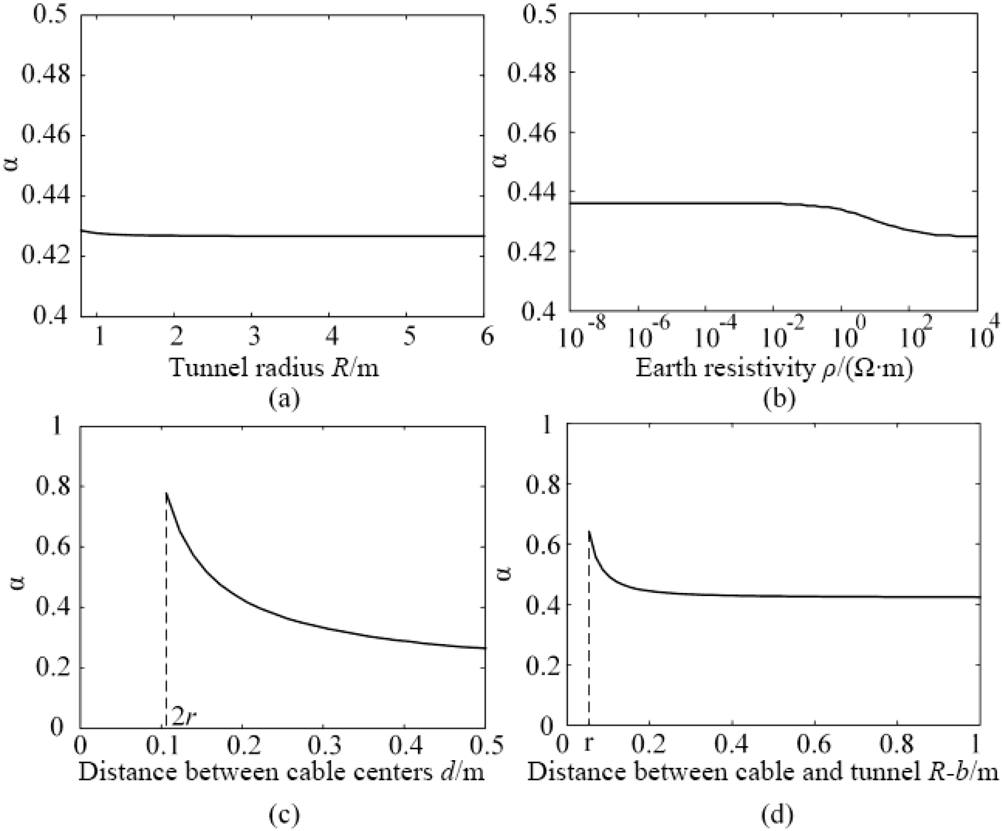
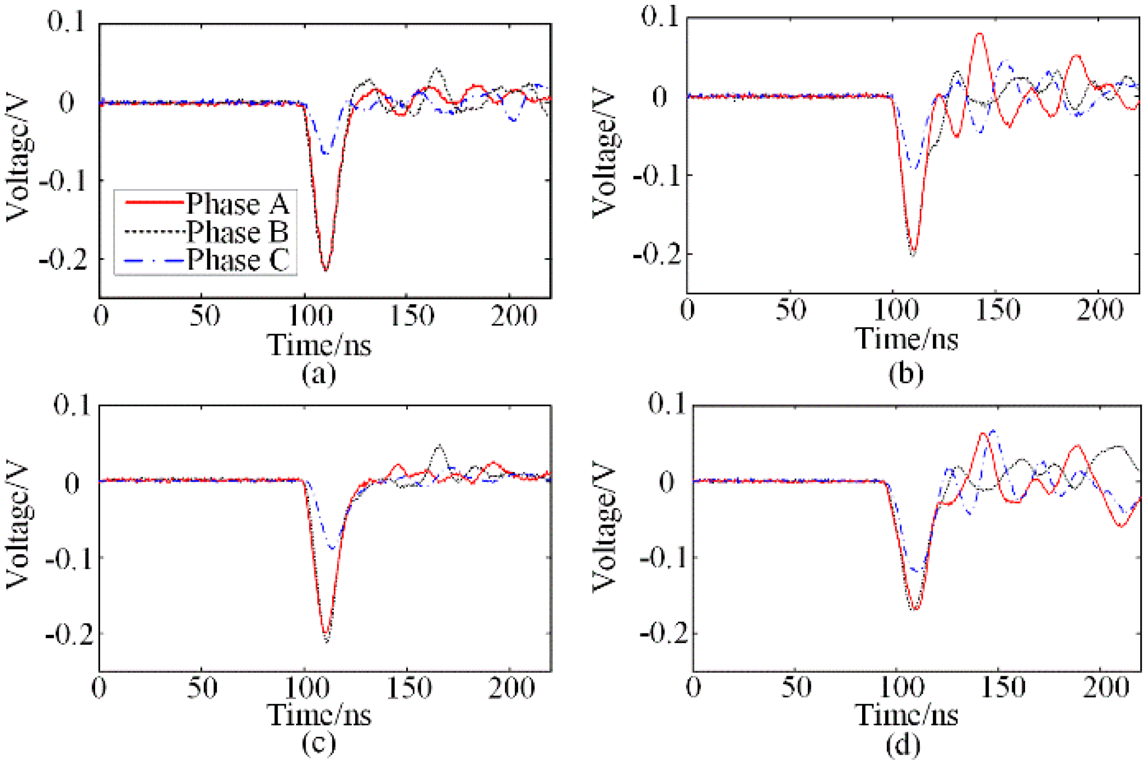
3.3. Influence of Cable Laying Parameters on Amplitude Distribution

In a three-phase tunnel-installed cable system, the amplitude distribution of the PD current in the adjacent cross-bonding wires is only related to the characteristic admittance ratio α. Therefore, by studying the influence of different laying parameters on α, including the tunnel radius R, the earth resistivity ρ, the cable center spacing, d and the distance from the cable to the inner wall of the tunnel R-b, different amplitude distribution characteristics under different conditions can be obtained. The 220 kV XLPE cable listed in Table 1 is selected as an example, and the typical laying parameters are also given as the reference condition.
As shown in Figure 5a,b the influence of the tunnel radius R and earth resistivity ρ on α is generally small, within about 5%. However, it can be seen from Figure 5c that the influence of the cable spacing d on α is very large. When the cables are getting closer to each other, α rises rapidly and reaches a maximum at 2 r. When the distance d increases, α approaches a fixed value. The variation of α in Figure 5d is similar to that in Figure 5c. When the distance from the cable to the inner wall of the tunnel R-b is r, that is, when the cable sheath is in direct contact with the inner wall of the tunnel, α reaches the maximum. As the cable moves away from the wall, α drops rapidly and tends to a fixed value.
The above results can be explained by the characteristic admittance model. If any two conductors in a three-phase cable system are treated as parallel conductors, the characteristic impedance of the two-conductor transmission line will be reduced and the characteristic admittance will increase when the distance between the conductors is reduced. The cable center spacing, d mainly affects Yss, and the distance to the inner wall of the tunnel R-b mainly affects Yse. Considering Equation (15), it can be seen that α will become larger in this case, and the ratio of Imajor/Iminor will increase accordingly.

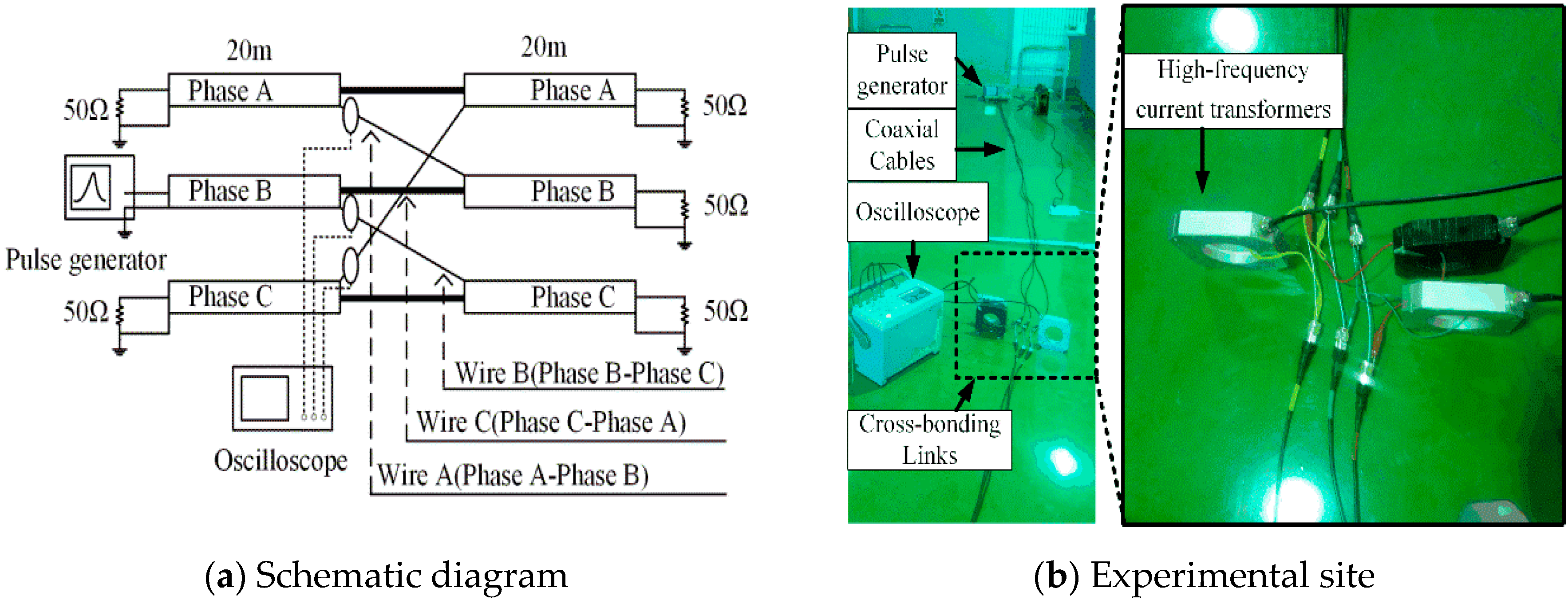
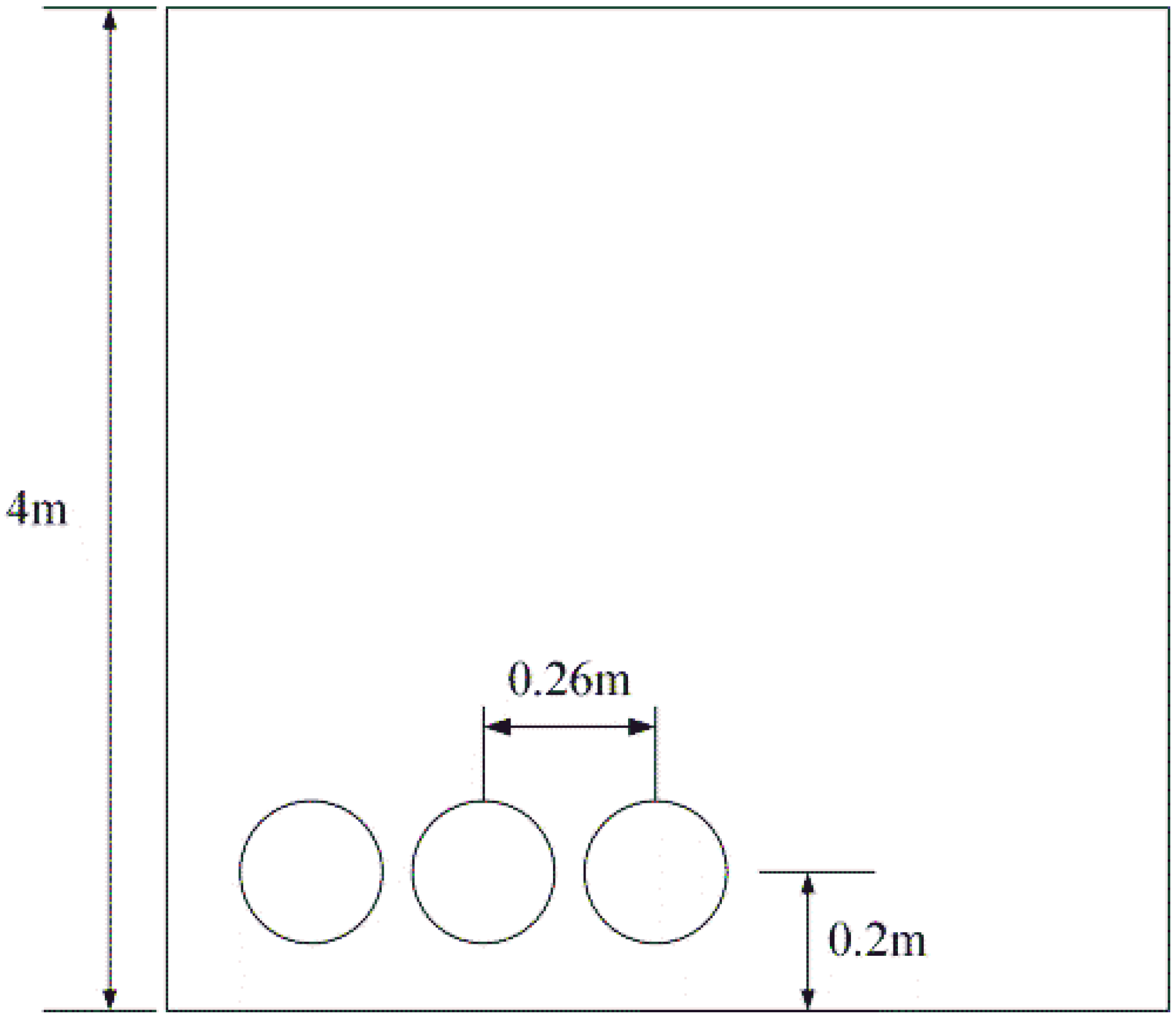
4. Experimental Verification

In order to verify the reliability of the characteristic admittance model and the accuracy of the PD signal amplitude distribution, RG223 coaxial cables were selected to simulate the three-phase cross-bonding cable system. In view of the fact that the tunnel radius R and the earth resistivity ρ have little effect on the signal amplitude distribution, the cable system was arranged in a shielded room for simulating the underground tunnel and reducing external interference. The equivalent radius of this tunnel was 4 m and the earth resistivity ρ is 1 × 10⁻⁷ Ω∙m. The parameters of the RG223 coaxial cable are shown in Table 2.
The total length of the cable system was 40 m. The cross-bonding connection was located in the middle of the cable system, 20 m on both sides. The PD pulse signal was a pulse generated by Tektronix AFG3101 (Beaverton, OR, USA) with an amplitude of 10 V and a rise time of 10 ns. The pulse signal was input through the end of the phase B cable. The remaining cable terminations were connected to 50 Ω resistive loads. The detected signal was recorded by the Keysight DSO6104 (Santa Rosa, CA, USA) oscilloscope. The bandwidth of the high-frequency current transformers was 1–50 MHz and the sampling rate of the oscilloscope was 2 GSa/s. The schematic diagram of the experimental setup and the experimental site are shown in Figure 6a,b, respectively.
Four different laying methods were adopted in the experiment, as shown in Figure 7. In modes a and b, the cables were closely arranged and the distance between adjacent cables was 5.35 mm. In modes c and d, the cables were arranged horizontally and the distance between adjacent cables was 0.1 m, with an equivalent geometric spacing of 0.126 m. In modes a and c, the cables were in direct contact with the tunnel wall and the distance to the wall was 2.675 mm, while the distance in modes b and d was 0.5 m. Each of the laying configuration was measured 5 times, and the results were highly consistent. Figure 8 shows one group of the measured results. The signals on the cross-bonding wires of phase A and B are similar while the signals in phase C are smaller. Besides, the polarities of the measured pulses are the same.
To further confirm the influence of the laying parameters, two kinds of methods were used to characterize the measured signal amplitude. One is to directly use the peak-to-peak value in the time domain, i.e., the difference between the positive peak and the negative peak of the time domain signal. The other method uses the average amplitude spectrum in the frequency domain, namely, calculates the average value of the Fourier transform of the time domain signal in the range of 3–30 MHz. Since the amplitudes of the phase A and phase B are not exactly equal in practice, the measured Imajor/Iminor ratio was calculated by dividing the average amplitude of the phase A and B by the amplitude of phase C. Table 3 shows that the Imajor/Iminor ratio of the average amplitude spectrum is closer to the theoretical value than the peak-to-peak value and the error is less than 10%. This is because the average amplitude spectrum excludes the influence of propagation delay and low-frequency amplitude spectrum, which is more in line with the premise of the theoretical definition. The advantage of the time-domain peak-to-peak is that it is simpler and more intuitive, and is suitable for applications where the requirement for accuracy is not very strict. One of the reasons for the error is that the RG223 coaxial cables used are semi-flexible cables with a small radius, so it is difficult for them to be tightly arranged. In the experiment, the cable center spacing, d in mode a and b was in fact slightly larger than 2r, and the distance R-b in modes a and c was slightly larger than r, so the results were generally smaller than the theoretical values.
In order to verify the effect of the cable center spacing, d on the amplitude distribution, we compared the average amplitude spectra of modes a and c (or modes b and d) in Table 3. It can be seen that the Imajor/Iminor ratio decreases from 4.04 to 2.52 when the equivalent center spacing, d increases from 5.35 mm to 126 mm. This change is consistent with the decreasing trend of the characteristic admittance ratio α in Figure 5c. In order to verify the influence of R-b on the amplitude distribution, the average amplitude spectra of modes a and b (or mode c and d) in Table 3 were compared. The Imajor/Iminor ratio decreases from 4.04 to 2.38 when R-b increases from 2.675 mm to 500 mm. This change also corresponds to the decreasing trend of the characteristic admittance ratio α in Figure 5d. It is known from Equation (17) that there is a proportional relationship between α and Imajor/Iminor. Therefore, the trend of the amplitude distribution caused by the change of the laying parameters is consistent with the analysis based on the characteristic admittance model, which verifies the accuracy of the model and its conclusion.

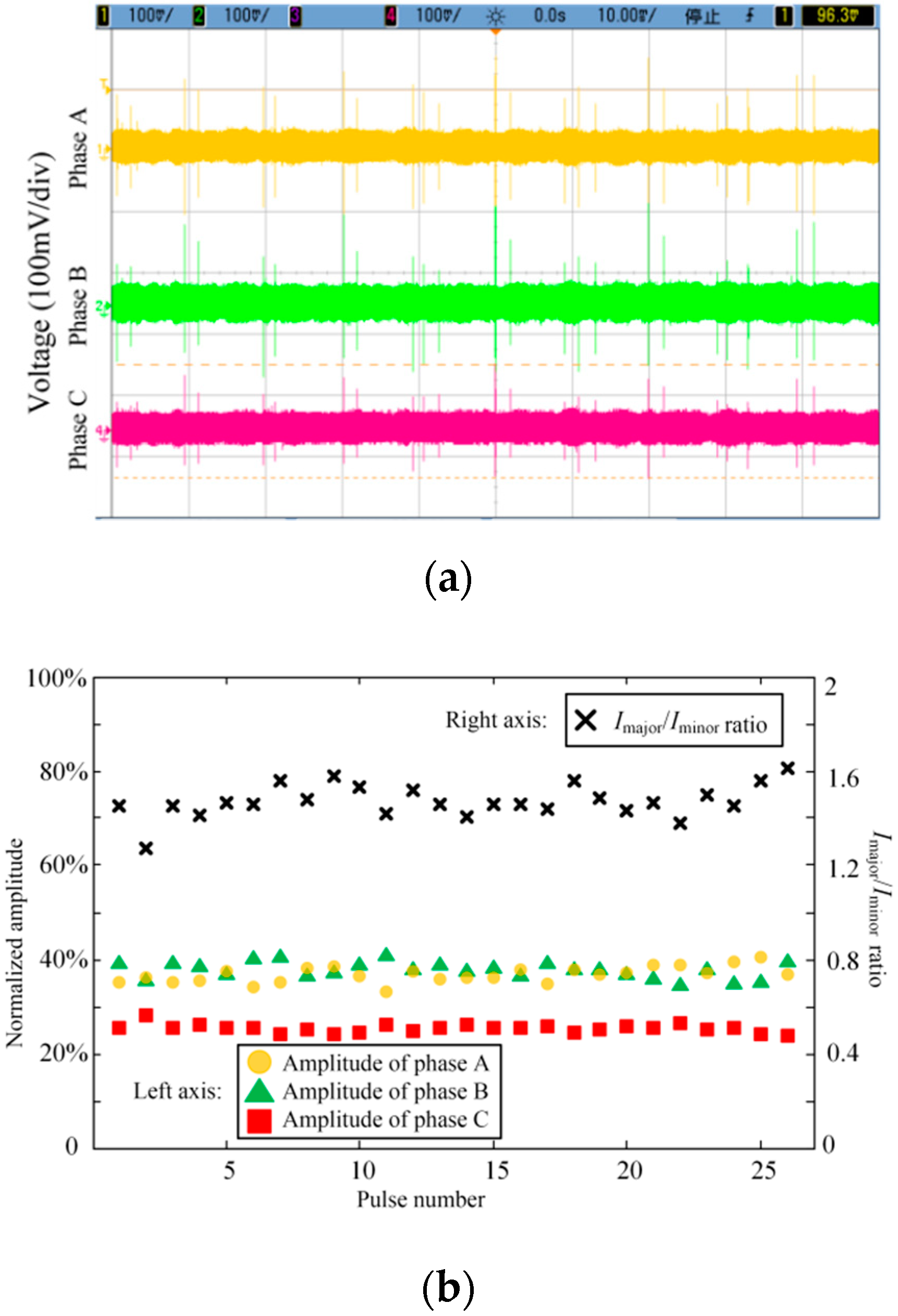
5. On-Site Measurements

A detection scheme combining the high-frequency current method and the ultra-high frequency (UHF) method was used for PD on-site detection of a 110 kV cable line. PD was confirmed and located in the cable termination of phase B by the time difference method [24]. The laying configuration of the cable line is sketched in Figure 9. The square tunnel can be regarded as a round tunnel with a radius of 2.3 m. The cable spacing is 0.26 m and the distance from the cable to the inner wall of the tunnel is 0.2 m. The earth resistivity is approximately 100 Ω∙m. The calculated Imajor/Iminor ratio is 1.52.
Figure 10 shows the high-frequency current signal of the # 1 cross-bonding wires adjacent to the termination. The signal was recorded at a sampling rate of 2 GSa/s by the Keysight DSO6104 oscilloscope after passing a 40 dB, 2 MHz high-pass amplifier.
Figure 10a shows that PD pulses existed on all the three-phase cross-bonding wires, and have a one-to-one correspondence in the time domain. The signals occurred in a 20-ms (50 Hz) cycle, and are distributed in both the positive and negative half cycle. The overall peak-to-peak values of the three-phase signals are 288 mV, 281 mV, and 184 mV, respectively. The Imajor/Iminor ratio is therefore approximately 1.55. A rectangular window was used to extract the pulses contained in the sampling period and 26 groups of PD pulse signals were obtained. After suppressing the background noise using wavelet denoising, the average amplitude spectrum was calculated and normalized with the sum of the three phases. The result is shown in Figure 10b. The data of each group are similar to each other, where the amplitudes of phase A and B are roughly equal and are all larger than the amplitude of phase C. The mean value of the Imajor/Iminor ratios is 1.47 and the standard deviation is 0.069, which is similar to that obtained from the peak-to-peak peak values.
Since the amplitudes of the signals on the cross-bonding wires of phase A and phase B are equal, the wires should be directly connected with the defective phase according to the analysis of Section 2.2. In combination with the structure of the cross-bonded cable system in Figure 1, the A-B phase and the B-C phase are connected by the cross-bonding wires of phase A and phase B respectively. The two cross-bonding wires are directly connected to phase B, so the PD source should be located in phase B, which is consistent with the actual situation.

6. Conclusions

Compared with the previous research on cross-boned systems, we used a more accurate expression, Tylavsky’s formulas, for tunnel modeling. Therefore, a simplified characteristic admittance model has been proposed for the first time. This model makes it possible to theoretically derive the amplitude distribution formula of the PD pulse current on the cross-bonding wires. Furthermore, we have studied the environmental parameters that affect the amplitude distribution of PD pulses, which is not considered in the previous research. The results are verified both by laboratorial experiments and on-site detection.
The amplitude distribution of the PD current on the cross-bonding wires is deduced using the characteristic admittance model. The results show that the polarities of the current signals at the adjacent cross-bonding joints are the same, and the proportional relationship of their amplitudes is only determined by the characteristic admittance ratio α. The laying parameters of the three-phase cable system will affect the amplitude distribution of the PD pulse current at the adjacent cross-bonding joints. Through the model analysis and experimental study, it is found that the amplitude distribution is mainly affected by the cable center spacing and the distance from the cable to the inner wall of the tunnel. On the other hand, the effect of the tunnel radius and earth resistivity is limited. The smaller the cable spacing, the closer the cable is to the inner wall of the tunnel, the greater the difference in the amplitudes of the signals on the cross-bonding wires.

Author Contributions

Data curation, X.C.; Formal analysis, Y.Q.; Funding acquisition, X.C.; Investigation, G.S.; Methodology, Y.Z.; Project administration, X.J.; Resources, Y.Z.; Software, X.C.; Supervision, Y.Q., H.W., G.S. and X.J.; Validation, Y.Q.; Visualization, H.W.; Writing—original draft, Y.Q.; Writing—review & editing, X.C.

Funding

This research was funded by the Project supported by Science and Technology Project of State Grid Zhejiang Electric Power Co., Ltd. (5211DS180035).

Conflicts of Interest

The authors declare no conflict of interest.

References

  1. Mahdipour, M.; Akbari, A.; Werle, P. Charge concept in partial discharge in power cables. IEEE Trans. Dielectr. Electr. Insul. 2017, 24, 817–825. [Google Scholar] [CrossRef]
  2. Chen, X.; Qian, Y.; Xu, Y.; Sheng, G.; Jiang, X. Energy estimation of partial discharge pulse signals based on noise parameters. IEEE Access 2016, 4, 10270–10279. [Google Scholar] [CrossRef]
  3. Mor, A.R.; Morshuis, P.H.F.; Smit, J.J. Comparison of charge estimation methods in partial discharge cable measurements. IEEE Trans. Dielectr. Electr. Insul. 2015, 22, 657–664. [Google Scholar] [CrossRef]
  4. Ahmed, N.H.; Srinivas, N.N. On-line partial discharge detection in cables. IEEE Trans. Dielectr. Electr. Insul. 1998, 5, 181–188. [Google Scholar] [CrossRef]
  5. Wild, M.; Tenbohlen, S.; Gulski, E.; Jongen, R. Basic aspects of partial discharge on-site testing of long length transmission power cables. IEEE Trans. Dielectr. Electr. Insul. 2017, 24, 1077–1087. [Google Scholar] [CrossRef]
  6. Eigner, A.; Rethmeier, K. An overview on the current status of partial discharge measurements on AC high voltage cable accessories. IEEE Electr. Insul. Mag. 2016, 32, 48–55. [Google Scholar] [CrossRef]
  7. Li, C.; Ma, G.; Qi, B.; Zhang, G.; Su, Q. Condition monitoring and diagnosis of high-voltage equipment in China-recent progress. IEEE Electr. Insul. Mag. 2013, 29, 71–78. [Google Scholar] [CrossRef]
  8. Wu, M.; Cao, H.; Cao, J.; Hai-Long, N.; Gomes, J.B.; Krishnaswamy, S.P. An overview of state-of-the-art partial discharge analysis techniques for condition monitoring. IEEE Electr. Insul. Mag. 2015, 31, 22–35. [Google Scholar] [CrossRef]
  9. Weissenberg, W.; Farid, F.; Plath, R. On-site PD detection at cross-bonding links of HV cables. In CIGRE Session; CIGRE: Paris, France, 2004. [Google Scholar]
  10. Xu, Y.; Gu, X.; Liu, B.; Hui, B.; Ren, Z.; Meng, S. Special requirements of high frequency current transformers in the on-line detection of partial discharges in power cables. IEEE Electr. Insul. Mag. 2016, 32, 8–19. [Google Scholar] [CrossRef]
  11. Babaee, A.; Shahrtash, S.M. On-line partial discharge defected phase selection and localization in cross-bonded single core cables. IEEE Trans. Dielectr. Electr. Insul. 2015, 22, 2995–3006. [Google Scholar] [CrossRef]
  12. Sheng, B.; Zhou, W.; Yu, J.; Meng, S.; Zhou, C.; Hepburn, D. On-line PD detection and localization in cross-bonded HV cable systems. IEEE Trans. Dielectr. Electr. Insul. 2014, 21, 2217–2224. [Google Scholar] [CrossRef]
  13. Wang, Z.; Liu, C.; Wang, Z.; Gao, C.; Sui, H. Application of capacitor sensor in PD detection at the three-phase cross-bonding link-system of XLPE Cable. In Proceedings of the 2010 Annual Report Conference on Electrical Insulation and Dielectric Phenomena (CEIDP), West Lafayette, IN, USA, 17–20 October 2010; pp. 1–3. [Google Scholar]
  14. Ametani, A. A general formulation of impedance and admittance of cables. IEEE Trans. Power Appar. Syst. 1980, PAS-99, 902–910. [Google Scholar] [CrossRef]
  15. Dommel, H.W. Underground cables. In EMTP Theory Book; Microtran Power System Analysis Corporation: Portland, OR, USA, 1992; pp. 150–192. [Google Scholar]
  16. Pollaczek, F. Uber das Feld einer unendlich langen wechselstromdurchflossen Einfachleitung. Elektr. Nachr. Tech. 1926, 3, 339–360. [Google Scholar]
  17. Tylavsky, D.J. Conductor impedance approximations for deep-underground mines. IEEE Trans. Ind. Appl. 1987, 4, 723–730. [Google Scholar] [CrossRef]
  18. Wu, M. Physical interpretation of impedance formulas for conductors enclosed in a cylindrical tunnel. IEEE Trans. Power Deliv. 2011, 26, 1354–1360. [Google Scholar]
  19. Chen, Y.; Gong, Q.; Chen, Y.; Cao, Y. Study of traveling wave at the sheath—Crossing point of high voltage power cable. High Volt. Eng. 2008, 32, 799–803. [Google Scholar]
  20. Wu, W.; Zhang, F. Power System Over-Voltage Numerical Calculation; Science Press: Beijing, China, 1989; pp. 155–174. [Google Scholar]
  21. Paul, C.R. Frequency-Domain analysis of multiconductor lines. In Analysis of Multiconductor Transmission Lines; John Wiley & Sons: Hoboken, NJ, USA, 2008; pp. 282–342. [Google Scholar]
  22. Lemke, E. Analysis of the partial discharge charge transfer in extruded power cables. IEEE Electr. Insul. Mag. 2013, 29, 24–28. [Google Scholar] [CrossRef]
  23. Ametani, A. Wave propagation characteristics of cables. IEEE Trans. Power Appar. Syst. 1980, PAS-99, 499–505. [Google Scholar] [CrossRef]
  24. Zhang, C.G.; Yao, L.; Qian, Y.; Huang, C.; Jiang, X. Application of HF/UHF joint partial discharge analysis to on-site power cable terminal detection. Electr. Power Autom. Equip. 2010, 30, 92–95. [Google Scholar]
Figure 1. High-frequency current method applied to a three-phase cross-bonded cable unit.
Applsci 09 04595 g001
Figure 2. Cross section of tunnel-installed cable system and structure of cable.
Applsci 09 04595 g002
Figure 3. Three-phase cable characteristic admittance model.
Applsci 09 04595 g003
Figure 4. Relationship between the real parts of the characteristic admittances and the frequency.
Applsci 09 04595 g004
Figure 5. Influence of laying parameters on characteristic admittance ratio α. (a) Tunnel radius. (b) Earth resistivity. (c) Distance between cable centers. (d) Distance between cable and tunnel.
Applsci 09 04595 g005
Figure 6. Experimental setup.
Applsci 09 04595 g006
Figure 7. Laying configurations of cables. (a) Triangle arrangement, on the ground. (b) Triangle arrangement, 0.5m above the ground. (c) Horizontal arrangement, on the ground. (d) Horizontal arrangement, 0.5m above the ground.
Applsci 09 04595 g007
Figure 8. Signals under different laying configurations. (a) Triangle arrangement, on the ground. (b) Triangle arrangement, 0.5m above the ground. (c) Horizontal arrangement, on the ground. (d) Horizontal arrangement, 0.5m above the ground.
Applsci 09 04595 g008
Figure 9. Laying configuration of the 110 kV cable line.
Applsci 09 04595 g009
Figure 10. On-site partial discharge (PD) pulses in cables and their amplitude distributions. (a) PD pulses displayed on the oscilloscope. (b) Amplitude distributions of the detected PD pulses.
Applsci 09 04595 g010
Table 1. Parameters of layout and cable.
Laying Parameters
Tunnel radius R/m2Earth resistivity ρ/(Ω∙m)100
Cable center spacing d/m0.2Cable distance from the tunnel wall R-b/m0.5
Cable parameters (YJLW03 127/220 1 × 1000)
Inner conductor radius r1/mm19Relative dielectric constant of insulation ε12.3
Insulation radius r2/mm46Relative dielectric constant of sheath ε23
Sheath radius r3/mm48.4Inner conductor resistivity ρ1/(Ω∙m)1.7 × 10−8
Cable radius r/mm53.4Sheath resistivity ρ2/(Ω∙m)2.1 × 10−8
Table 2. Parameters of RG223 coaxial cables.
Inner Conductor Radius r1/mm0.45Insulating Layer Relative Dielectric Constant ε12.3
Insulation radius r2/mm1.475Sheath relative dielectric constant ε23
Metal shielding radius r3/mm2.1Inner conductor resistivity ρ1/(Ω∙m)1.75 × 10−8
Cable radius r/mm2.675Metal shielding resistivity ρ2/(Ω∙m)1.75 × 10−8
Table 3. Measured Signal Amplitudes and the Ratio of Imajor/Iminor.
Laying ConfigurationPeak-to-Peak Value Average Amplitude SpectrumImajor/Iminor
Phase APhase BPhase CPhase APhase BPhase CPeak-to-Peak ValueAverage Amplitude SpectrumTheoretical Value
Mode a0.2390.2590.0940.1370.1380.0342.654.044.42
Mode b0.2690.2360.1380.1190.1240.0510.1832.382.64
Mode c0.2270.2630.1090.1230.1240.0492.252.522.59
Mode d0.2330.2160.1870.1190.1190.0831.201.431.41

