1. Introduction
The stability of local slopes is a critical issue that needs to be meticulously investigated due to their great impact on the adjacent engineering projects (excavation and transmission roads, for instance). In addition to that, slope failures cause great psychological damage (e.g., the loss of property and human life) all over the world every year. In Iran, for example, based on a rough estimation announced by the Iranian Landslide Working Party (2007), 187 people have been killed every year by slope failure in this country [
1]. The saturation degree, as well as other intrinsic properties of the soil, significantly affect the likelihood of slope failure [
2,
3]. Up to now, many scientists have intended to provide effective modeling for slope stability problems. Some drawbacks of traditional methods, such as the necessity of using laboratory equipment and the high level of complexity prevent them from being a simply used solution [
4]. Moreover, they cannot be used as a comprehensive solution due to their limitation in investigating a specific slope condition (e.g., slope angle, height, groundwater level, soil properties, etc.). Different types of limit equilibrium methods (LEMs), finite element model (FEM), and numerical solutions have been extensively employed for the engineering problem [
5,
6,
7,
8]. Development of design charts has been investigated for years in order to provide a reliable tool for slope stability assessment [
9]. However, this approach is not devoid of defects either. Generating an efficient design chart requires consuming a lot of time and cost. Furthermore, determining the precise mechanical parameters is a difficult task [
10,
11]. Hence, the application of artificial intelligence techniques is more highlighted due to their quick performance and sufficient accuracy. The prominent superiority of these approaches is that they are able to detect the non-linear relationship between the target parameter(s) and its key factors. Also, ANN can be implemented using any determined number of hidden nodes [
12,
13]. For example, the suitable efficiency of an artificial neural network (ANN) [
14,
15,
16] and a support vector machine (SVM) [
17] has been proven in many geotechnical studies. After reviewing the literature, the complexity of the slope stability problem is evident. What makes the issue even more complicated and critical is constructing various structures in the vicinity of slopes (i.e., indicating a noticeable number of loads applied on a rigid footing). The amount of surcharge and the distance from the slope’s crest are two parameters influencing the stability of the purposed slope [
18]. This encouraged scholars to present an equation to calculate the factor of safety (FOS) of pure slopes or the slopes receiving a static load [
19,
20,
21,
22,
23]. Prior to this study, Chakraborty and Goswami estimated the FOS for 200 slopes with different geometric and shear strength parameters using the multiple linear regression (MLR) and ANN models. They also compared the obtained results with an FEM model, and an acceptable rate of accuracy was obtained for both applied models. In this research, ANN outperformed MLR. Also, Pei et al. [
23] effectively used the random forest (RF) and regression tree predictive models in functional soil-landscape modeling for regionalizing the depth of the failure plane and soil bulk density. They developed a classification for detecting the safe and hazardous slopes by means of FOS calculations. In some cases, the random forest and logistic regression techniques were implemented for a susceptibility modeling of a shallow landslide phenomena. They found that applied models have an excellent capability for this work. The SVM model synthesized by a minimal sequential optimization (SMO) algorithm has been used for surface grinding quality [
24] and many medical classifications [
25]. Also, a radial basis function regression (RBFR) has been successfully employed in genetics for predicting quantitative traits [
26], and in agriculture for the discrimination of cover crops in olive orchards [
27]. Another machine learning method that is used in the current paper is lazy k-nearest neighbor (IBK) tool. As the name implies, the lazy learning is the essence of this model and has shown good performance for many fields, such as spam e-mail filtering [
28] and land cover assessment [
29].
Though plenty of effort has been carried out to employ various soft computing tools for evaluating the stability of slopes [
30,
31], no prior study was found to address a comprehensive comparison of the applicability of the mentioned models within the same paper. Therefore, in this paper, we investigated the efficiency of seven machine-learning models (i.e., in their optimal structure), namely multiple linear regression (MLR), multi-layer perceptron (MLP), radial basis function regression (RBFR), improved support vector machine using sequential minimal optimization algorithm (SMO-SVM), lazy k-nearest neighbor (IBK), random forest (RF), and random tree (RT), for appraising the stability of a cohesive soil slope. Furthermore, since the authors did not find any former application of IBK, RBFR, or SMO-SVM for estimating the FOS of the slope, the further novelty of the current study can be announced as applying the mentioned models for the first time in this field. In this regard, the Optum G2 software was used to give the FOS of 630 different slopes. Four conditioning factors that affected the values of FOS were chosen: undrained shear strength (Cu), slope angle (β), setback distance ratio (b/B), and applied surcharge on the shallow foundation installed over the slope (w). The utilized models were implemented in Waikato Environment for Knowledge Analysis (WEKA) software (stable version, Waikato, New Zealand) using the training dataset (i.e., 80% of the entire dataset). Then, the performance of each model was evaluated using testing samples (i.e., 20% of the entire dataset). The results were presented by means of several statistical indices. In the end, a new classification was carried out based on different degrees of stability to evaluate and compare the results of the models used. In addition, the design solution charts were developed using the outputs of the most efficient model.
2. Data Collection and Methodology
To acquire a reliable dataset, the use of a single-layer slope was proposed. It was supposed that a purely cohesive soil, which only had undrained cohesive strength (C
u), comprises the body of this slope (see
Figure 1). The main factors that affect the strength of the slope against the failure (i.e., FOS) were considered to be the slope angle (β), setback distance ratio (b/B), and applied surcharge on the footing installed over the slope (w). These parameters are illustrated in
Figure 1. To calculate the FOS, Optum G2 software, which is a comprehensive finite element program for geotechnical stability and deformation analysis, was used [
32]. Regarding the possible values for the strength of the soil (C
u) and applied surcharge (w), different geometries of the slope (β), and displacements of the rigid foundation (b/B), 630 possible stages were modelled and analyzed in Optum G2 to calculate the FOS of each stage as the output. In the modeling process, the mechanical parameters of Poisson’s ratio, soil unit weight, and internal friction angle were assigned to be 0.35, 18 kN/m
3, and 0°, respectively. Also, Young’s modulus (E) was varied for every value of C
u. In this sense, E was set to 1000, 2000, 3500, 5000, 9000, 15,000, and 30,000 kPa for the following respective values of C
u: 25, 50, 75, 100, 200, 300, and 400 kPa.
The graphical relationship between the FOS and its influential factors is depicted in
Figure 2a–d. In these charts, C
u, β, b/B, and
w are each placed on a horizontal (x) axis versus the obtained FOS (i.e., from Optum G2 analyses) on the vertical (y) axis. The FOS ranges within [0.8, 28.55] for all graphs. Not surprisingly, as a general view, the slope experienced more stability when a higher value of C
u was assigned to the soil (see
Figure 2a). As
Figure 2b,d illustrate, the parameters β (5°, 30°, 45°, 60°, and 75°) and w (50, 100, and 150 KN/m
2) were inversely proportional to the FOS. This means the slope was more likely to fail when the model was performed with higher values of β and w. According to
Figure 2c, the FOS did not show any significant sensitivity to the b/B ratio changes (0, 1, 2, 3, 4, and 5).
Table 1 provides an example of the dataset used in this paper. The dataset was randomly divided into training and testing sub-groups, with the respective ratios of 0.8 (504 samples) and 0.2 (126 samples), based on previous studies [
33]. Note that the training samples were used to train the MLR, MLP, RBF, SMO-SVM, IBK, RF, and RT models, and their performance was validated by means of the testing dataset. The 10-fold cross-validation process was used to select the training and test datasets (
Figure 3). The results achieved were based on the best average accuracy for each classifier using 10-fold cross-validation (TFCV) based on the 20%/80% training/test split. In short, TFCV (which is a specific operation of k-fold cross-validation) divided our dataset into 10-partitions. In the first fold, a specific set of eight partitions of the data was used to train each model, whereas two partitions were used for testing. The accuracy for this fold was then indicated. This complied with using a various 20%/80% combinations of the data for training/testing, whose accuracy is also indicated. In the end, after all 10 folds were finished, the overall average accuracy was calculated [
34,
35].
In the following, the aim was to evaluate the competency of the applied models through a novel procedure based on the classification. In this sense, the actual values of the safety factor (i.e., obtained from the Optum G2 analysis) were stratified into five stability classes. The safety factor values varied from 0.8 to 28.55. Hence, the classification was carried out with respect to the extents given below (
Table 2):
As previously expressed, this study aimed to appraise the applicability of the seven most-employed machine learning models, namely multiple linear regression (MLR), multi-layer perceptron (MLP), radial basis function regression (RBFR), improved support vector machine using sequential minimal optimization algorithm (SMO-SVM), lazy k-nearest neighbor (IBK), random forest (RF), and random tree (RT), toward evaluating the stability of a cohesive slope. For this purpose, the factor of safety (FOS) of the slope was estimated using the above-mentioned methods. Four slope stability effective factors that were chosen for this study were the undrained shear strength (C
u), slope angle (β), setback distance ratio (b/B), and applied surcharge on the footing installed over the slope (w). To prepare the input target dataset, 630 different stages were developed and analyzed in Optum G2 finite element software. As a result of this process, a FOS was derived for each performed stage. To create the required dataset, the values of C
u, β, b/B, and
w were listed with the corresponding FOS. In the following, 80% of the prepared dataset (training phase consisting of 504 samples) was randomly selected for training the utilized models (MLR, MLP, RBFR, SMO-SVM, IBK, RF, and RT), and the effectiveness of them was evaluated by means of the remaining 20% of the dataset (testing phase consisting of 126 samples). The training process was carried out in WEKA software, which is an applicable tool for classification utilization and data mining. Note that many scholars have employed WEKA before for various simulating objectives [
36,
37]. To evaluate the efficiency of the implemented model, five statistical indices, namely the coefficient of determination (R
2), mean absolute error (
MAE), root mean square error (
RMSE), relative absolute error (
RAE in %), and root relative squared error (
RRSE in %), were used to develop a color intensity ranking and present a visualized comparison of the results. It should be noted that these criteria have been broadly used in earlier studies [
38]. Equations (1)–(5) describe the formulation of R
2,
MAE,
RMSE,
RAE, and
RRSE, respectively.
In all the above equations, Yi observed and Yi predicted stand for the actual and predicted values of the FOS, respectively. The term S is the indicator of the number of data points and is the average of the actual values of the FOS. The outcomes of this paper are presented in various ways. In the next part, the competency of the applied models (i.e., MLR, MLP, RBFR, SMO-SVM, IBK, RF, and RT) for the approximation of FOS is extensively presented, compared, and discussed.
2.1. Machine Learning Techniques
The present research outlines the application of various machine-learning-based predictive models, namely multiple linear regression (MLR), multi-layer perceptron (MLP), radial basis function regression (RBFR), improved support vector machine using sequential minimal optimization algorithm (SMO-SVM), lazy k-nearest neighbor (IBK), random forest (RF), and random tree (RT), in slope stability assessment. Analysis was undertaken using WEKA software [
39]. The mentioned models are described below.
2.1.1. Multiple Linear Regression (MLR)
Fitting a linear equation to the data samples (
Figure 4) is the essence of the multiple linear regression (MLR) model. It tries to reveal the generic equation between two or more explanatory (independent) variables and a response (dependent) variable. Equation (6) defines the general equation of the MLR [
40]:
where
x and
y are the independent and dependent variables, respectively. The terms
ρ0,
ρ1, ...,
ρs indicate the unknown parameters of the MLR. Also,
χ is the random variable in the MLR generic formula that has a normal distribution.
The main task of MLR is to forecast the unknown terms (i.e.,
ρ0,
ρ1, ...,
ρs) of Equation (6). By applying the least-squares technique, the practical form of the statistical regression method is represented as follows [
40]:
In the above equation
p0,
p1, ...,
ps are the approximated regression coefficients of
ρ0,
ρ1, ...,
ρs, respectively. Also, the term
μ gives the estimated error for the sample. Assuming the
μ is the difference between the real and modelled
y, the estimation of
y is performed as follows
2.1.2. Multi-Layer Perceptron (MLP)
Imitating the human neural network, an artificial neural network (ANN) was first suggested by McCulloch and Pitts [
41]. The non-linear rules between each set of inputs and their specific target(s) can be easily revealed using ANN [
42]. Many scholars have used different types of ANN to model various engineering models [
14,
16,
20,
38,
43,
44]. Despite the explicit benefits of ANNs, the most significant disadvantages of them lie in being trapped in their local minima and overfitting. A highly connected pattern forms the structure of an ANN. A multi-layer perceptron is one of the most prevalent types of this model. A minimum of three layers is needed to form the MLP structure. Every layer contains a different number of so-called computational nodes called “neurons.”
Figure 5a illustrates the schematic view of the MLP neural network that was used in this study. This network had two hidden layers comprising 10 neurons each. Every line in this structure is indicative of an interconnection weight (W). A more detailed view of the performance of a typical neuron is shown in
Figure 5b:
Note that, in
Figure 1b, the parameter
hj is calculated as follows:
where the terms
W,
X, and
b stand for the weight, input, and bias of the utilized neuron. Also, the function
f denotes the activation function of the neuron that is applied to produce the output.
2.1.3. Radial Basis Function Regression (RBFR)
Th radial basis function (RBF) approach (shown in
Figure 6) was first presented by Broomhead and Lowe [
45] for exact function interpolation [
46]. The RBF regression model attempts to fit a set of local kernels in high-dimensional space to solve problems [
45,
47,
48]. The position of noisy instances is considered for executing the fitting. The number of purposed kernels is often estimated using a bath algorithm.
The RBF regression performs through establishing an expectation function with the overall form of Equation (10):
where ‖
x‖ represents the Euclidean norm on
x and
is a set of
m RBFs, which are characterized by their non-linearity and being constant on
x. Also, the regression coefficient is denoted by
ri in this formula. Every training sample (i.e.,
xi) determines a center of the RBFs. In other words, the so-called function “radial” is impressively dependent on the distance (
ψ) between the center (
xi) and the origin (
x) (i.e.,
) The Gaussian
k(
r) =
exp(−
σψ2), for
ψ ≥ 0 [
49,
50]; the multi-quadric
[
51]; and the thin-plate-spline
k(
r) =
ψ2logψ [
52,
53] functions are three extensively applied examples of the function
k(
x) following the RBF rules.
2.1.4. Improved Support Vector Machine using Sequential Minimal Optimization Algorithm (SMO-SVM)
Support Vector Machine (SVM)
Insulating different classes is the pivotal norm during the performance of the support vector machine (SVM). This happens through detecting the decision boundaries. SVMs have been shown to have a suitable accuracy in various classification problems when dealing with high-dimensional and non-separable datasets [
54,
55,
56]. Theoretically, SVMs act according to statistical theories [
57] and aim to transform the problem from non-linear to linear future spaces [
58]. More specifically, assessing the support vectors that are set at the edge of the module descriptors will lead to locating the most appropriate hyperplane between the modules. Note that guiding cases that could not be a support vector are known as neglected vectors [
59]. The graphical description of the mentioned procedure is depicted in
Figure 7:
In the SVMs, the formulation of the hyperplane (i.e., the decision surface) is as follows:
where
lj,
x, and
fj represent the Lagrange coefficient, the vector that is drawn from the input space, and the
jth output, respectively. Also,
K(
x,
xi) is indicative of the inner-product kernel (i.e., the linear kernel function) and operates as given in Equation (12):
where
x and
xj stand for the input vector and input pattern related to the
jth instance, respectively.
The vector
w and the biasing threshold
b are obtained from Equations (13) and (14) [
60]:
Also,
Q(
l), which is a quadratic function (in
li), is given using the following formula:
Sequential Minimal Optimization (SMO)
Sequential minimal optimization (SMO) is a simple algorithm that was used in this study to improve the performance of the SVM. When corresponding the linear weight vector to the optimal values of
li using SMO, adding a matrix repository and establishing a repetitive statistical is not required. Every pair of Lagrange multiplier, such as
l1 and
l2 (
l1 <
l2), vary from 0 to
C. During the SMO performance, the
l2 is first computed. The extent of the transverse contour fragment is determined based on the obtained
l2 [
60]. If the targets
f1 and
f2 are equal, the subsequent bounds apply to
l1 (Equation (10)); otherwise, they apply to
l2. Equation (16) defines the directional minimum along with the contour fragment acquired using SMO:
where
Ej is the difference between the
jth SMV output and the target. The parameter
λ stands for an unbiased function and is given by the following equation:
In the following, the
l2′ clipped to the range [
A,
B]:
Finally, l1 and l2 are moved to the bound with the lowest unbiased function.
After optimizing the Lagrange multipliers, SVM is eligible to give the output
f1 using the threshold
b1, if 0 <
l1 <
C [
60]. Equations (22) and (23) show the way that
b1 and
b2 are calculated:
2.1.5. Lazy k-Nearest Neighbor (IBK)
In the lazy learning procedure, the generalization of the training sample commences with producing a query and learners do not tend to operate until the classification time. Generating the objective function through a local estimation can be stated as the main advantage of the models associated with lazy learning. One of the most prevalent techniques that follow these rules is the k-nearest neighbor algorithm [
61]. Multiple problems can be simulated with this approach due to the local estimation accomplished for all queries to the system. Moreover, this feature causes the capability of such systems to work, even when the problem conditions change [
62,
63]. Even though lazy learning has been shown to have a suitable quickness for training, validation takes place over longer time. Furthermore, since the complete training process is stored in this method, a large space is required for the k-nearest neighborhood (IBK) classifier as a non-parametric model that has a good background for classification and regression utilization [
61]. The number of nearest neighbors can be specified exactly in the object editor or set automatically through applying cross-validation to a certain upper bound. IBK utilizes various search algorithms (that are linear by default) to expedite finding the nearest neighbors. Also, the default function for evaluating the position of samples is the Euclidean distance, which can be substituted by Minkowski, Manhattan, and Chebyshev distance functions [
64]. As is well-discussed in References [
62,
65], the distance from the validation data can be a valid criterion to weight the estimations from more than one neighbor. Note that altering the oldest training data with new possible samples takes place by determining a window size. It helps to have a constant number of samples [
66].
2.1.6. Random Forest (RF)
The random forest (RF) is a capable tool used for classification problems [
67]. RF follows the ensemble learning rules by employing several classification trees [
68]. In this model, showing better results than entire individual trees (i.e., the better performance of an ensemble of classification trees) entails a greater than random accuracy, as well as the variety of the ensemble members [
69]. During the FR implementation, it aims to change the predictive relations randomly to increase the diversity of trees in the utilized forest. The development of the forest necessitates the user to specify the values of the number of trees (t) and the number of variables that cleave the nodes (g). Note that either categorical or numerical variables are eligible for this task. The parameter
t needs to be high enough to guarantee the reliability of the model. The unbiased estimation of the generalization error (GE), called the out-of-bag (OOB) error is obtained, when the random forest is being formed. Breiman [
67] showed that a limiting value of GE is produced by RF. The OOB error is computed using the ratio of the misclassification error over the total out-of-bag elements. RF attempts to appraise the prominence of the predictive variables through considering the increase of the OOB error. This increment is caused by permuting the OOB data for the utilized variable, while other variables are left without any change. It must be noted that the prominence of the predictive variable rises as the OOB error increases [
70]. Since each tree is counted as a completely independent random case, the affluence of random trees can lead to reducing the likelihood of overfitting. Note that this can be considered a key advantage of RF. This algorithm can automatically handle the missing values due to its suitable resistance against the outliers when making predictions.
2.1.7. Random Tree (RT)
Random trees (RT) symbolize a supervised classification model first introduced by Leo Breiman and Adele Cutler [
67]. Similar to RF, ensemble learning forms the essence of RT. In this approach, many learners who operate individually are involved. To develop a decision tree, a bagging idea is used to provide a randomly chosen group of samples. The pivotal difference between a standard tree and random forest (FR) is found in the splitting of the node. In RF, this is executed using the best among the subgroup of predictors, while a standard tree uses the elite split among all variables. The RT is an ensemble of tree forecasters (i.e., forest) and can handle both regression and classification utilizations. During the RT execution, the input data are given to the tree classifier. Every existing tree performs the classification of the inputs. Eventually, the category with the highest frequency is the output of the system. This is noteworthy because the training error is calculated internally; none of cross-validation and bootstraps are needed to estimate the accuracy of the training stage. Note that the average of the responses of the whole forest members is computed to produce the output of the regression problems [
71]. The error of this scheme is a proportion of the number of misclassified vectors to all vectors in the original data.
3. Results and Discussion
The calculated values of R
2,
MAE,
RMSE,
RAE, and
RRSE for estimating the FOS are tabulated in
Table 3 and
Table 4 for the training and testing datasets. Also, the total ranking obtained for the models is featured in
Table 5. A color intensity model is given to denote the quality of results graphically. A red collection is considered for particular results. A higher value of R
2 and lower
MAE,
RMSE,
RAE, and
RRSE are represented using a more intense red color. In the last column, the intensity of a green collection is supposed to be inversely proportional to the ranking gained by each model.
At a glance, RF could be seen to be the outstanding model due to its highest score. However, based on the acquired R
2 for the training (0.9586, 0.9937, 0.9948, 0.9529, 1.000, 0.9997, and 0.9998, calculated for MLR, MLP, RBFR, SMO-SVM, IBK, RF, and RT, respectively) and testing (0.9649, 0.9939, 0.9955, 0.9653, 0.9837, 0.9985, and 0.9950, respectively) datasets, an acceptable correlation could be seen for all models. Referring to the
RMSE (28.4887, 1.7366, 0.7131, 0.6231, 1.9183, 0.00, 0.1486, and 0.1111) and
RRSE (11.6985%, 10.2221%, 31.4703%, 0.0000%, 2.4385%, and 1.8221%) obtained for the training dataset, the IBK predictive model presented the most effective training compared to other models. Also, RT and RF could be seen as the second- and third-most accurate models, respectively, in the training stage. In addition, RBFR outperformed MLP, MLR, and SMO-SVM (as shown in
Table 3).
The results for evaluating the performance of the models used are available in
Table 4. Despite this fact that IBK showed an excellent performance during the training phase, a better validation was achieved using the RF, RBFR, RT, and MLP methods in this part. This claim can be proved by the obtained values of R
2 (0.9649, 0.9939, 0.9955, 0.9653, 0.9837, 0.9985, and 0.9950),
MAE (1.1939, 0.5149, 0.3936, 1.0360, 0.8184, 0.2152, and 0.3492) and
RAE (24.1272%, 10.4047%, 7.9549%, 20.9366%, 16.5388%, 4.3498%, and 7.0576%) for MLR, MLP, RBFR, SMO-SVM, IBK, RF, and RT, respectively. Respective values of 0.9985, 0.2152, 0.3312, 4.3498%, and 5.5145% computed for R
2,
MAE,
RMSE,
RAE, and
RRSE indices show that the highest level of accuracy in the validation phase was achieved by RF. Similar to the training phase, the lowest reliability was achieved by the SVM and MLR models, compared to the other utilized techniques.
Furthermore, a comprehensive comparison (regarding the results of both the training and testing datasets) of applied methods is conducted in
Table 5. In this table, considering the assumption of individual ranks obtained for each model (based on the R
2,
MAE,
RMSE,
RAE, and
RRSE in
Table 3 and
Table 4), a new total ranking is provided. According to this table, the RF (total score = 60) was the most efficient model in the current study due to its good performance in both the training and testing phases. After RF, RT (total score = 57) was the second-most reliable model. Other employed methods including IBK (total score = 50), RBFR (total score = 48), and MLP (total score = 35) were the third-, fourth-, and fifth-most accurate tools, respectively. Also, the poorest estimation was given by the SMO-SVM and MLR approaches (total score = 15 for both models).
Application of multiple linear regression (MLR), multi-layer perceptron (MLP), radial basis function regression (RBFR), improved support vector machine using sequential minimal optimization algorithm (SMO-SVM), lazy k-nearest neighbor (IBK), random forest (RF), and random tree (RT) was found to be viable for appraising the stability of a single-layered cohesive slope. The models that use ensemble learning (i.e., RF and RT) outperformed the models that are based on lazy-learning (IBK), regression rules (MLR and RBFR), neural learning (MLP), and statistical theories (SMO-SVM). Referring to the acquired total scores (the summation of scores obtained for the training and testing stages) of 15, 35, 48, 15, 50, 60, and 57 for MLR, MLP, RBFR, SMO-SVM, IBK, RF, and RT, respectively, shows the superiority of the RT algorithm. After that, RT, IBK, and RBFR were shown to have an excellent performance when estimating the FOS. Also, satisfying reliability was found for the MLP, SMO-SVM, and MLR methods. Based on the results obtained for the classification of the risk of failure, the closest approximation was achieved using the RF, RT, IBK, and SMO-SVM methods. In this regard, 14.60% of the dataset was assorted as hazardous slopes (i.e., “unstable” and “low stability” categories). This value was estimated as 18.25%, 12.54%, 12.70%, 14.76%, 14.60%, 13.81%, and 14.13% by the MLR, MLP, RBFR, SMO-SVM, IBK, RF, and RT models, respectively.
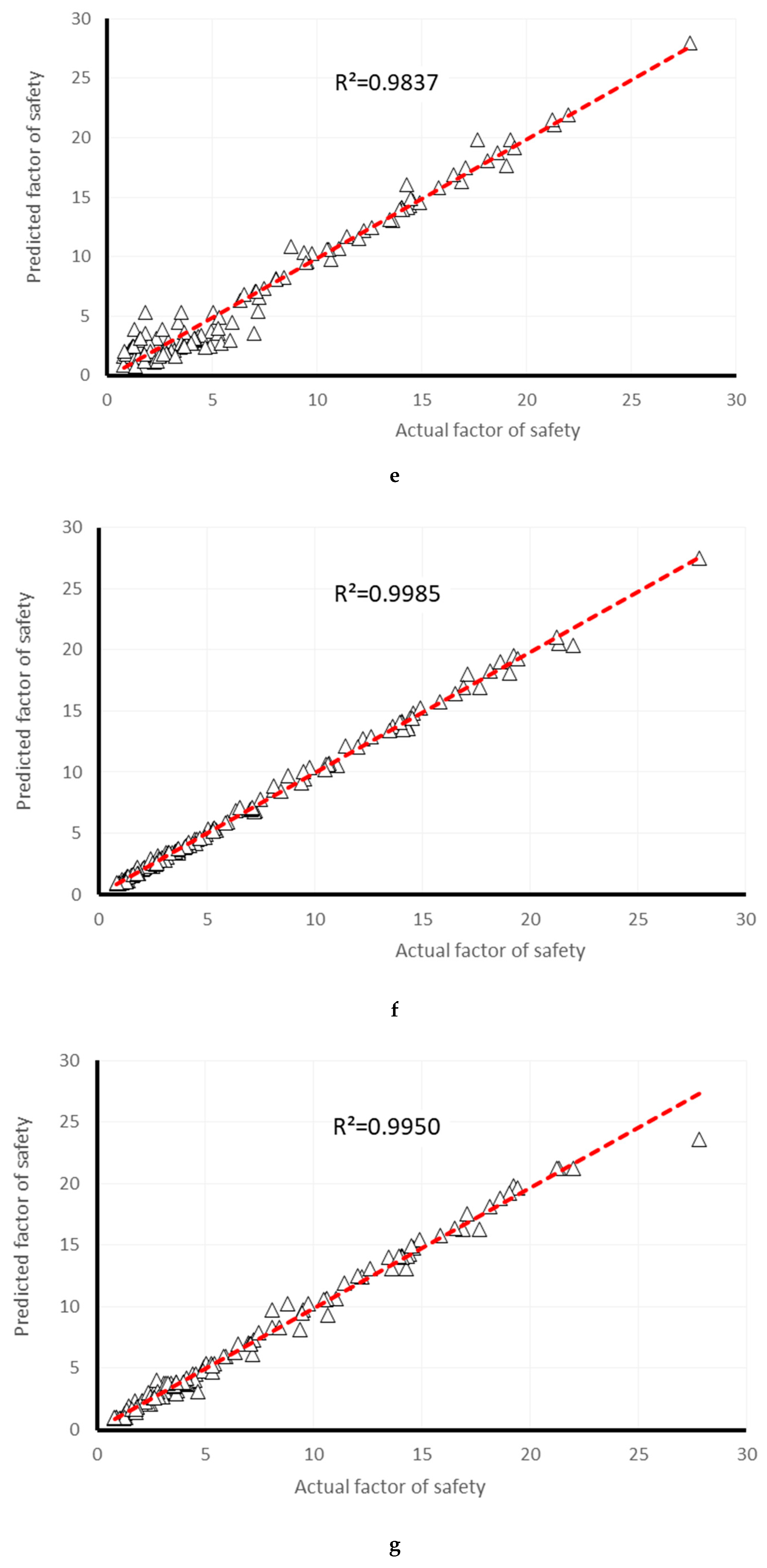
It is well established that the best relationship between the data shown on the horizontal and vertical axis is demonstrated using the line x = y, in the regression chart. According to
Figure 8 and
Figure 9, the IBK produced the closest outputs to the actual values of the safety factor in the training phase (R
2 = 1). Also, the highest correlation was achieved by the RF outputs for the testing data (R
2 = 0.9985). A higher scattering in samples, observed for MLR (R
2 = 0.9586 and 0.9649) and SMO-SVM (R
2 = 0.9529 and 0.9653) predictions indicates a lower sensitivity of these models in both the training and testing datasets.
The percentage of each stability class (i.e., the number of safety factor values in the utilized class over the whole number of data points) was calculated. The results of this part are depicted in the form of a column chart in
Figure 10.
In addition, the regression between the actual and estimated values of FOS is depicted in
Figure 6 and
Figure 7 for the training and testing data.
Based on this chart, more than half of the safety factor values indicated a safe condition for the examined slope. Almost all employed models showed a good approximation for the classification of the risk of failure. Considering the categories “unstable” and “low stability” as the dangerous situation of the slope (i.e., the slope was more likely to fail with these safety factors), a total of 14.60% of the dataset was assorted as being dangerous. This value was estimated as 18.25%, 12.54%, 12.70%, 14.76%, 14.60%, 13.81%, and 14.13% by the MLR, MLP, RBFR, SMO-SVM, IBK, RF, and RT models, respectively.
where the parameters Z
1, Z
2, …, Z
10 are shown in
Table 6 and weight and biases tabulated in
Table 7:
where the parameters Y
1, Y
2, …, Y
10 are in
Table 7.
4. Conclusions
In the past, many scholars have investigated the slope failure phenomenon due to its huge impact on many civil engineering projects. Due to this, many traditional techniques offering numerical and finite element solutions have been developed. The appearance of machine learning has made these techniques antiquated. Therefore, the main incentive of this study was to evaluate the proficiency of various machine-learning-based models, namely multiple linear regression (MLR), multi-layer perceptron (MLP), radial basis function regression (RBFR), improved support vector machine using sequential minimal optimization algorithm (SMO-SVM), lazy k-nearest neighbor (IBK), random forest (RF), and random tree (RT), in estimating the factor of safety (FOS) of a cohesive slope. To provide the required dataset. Optum G2 software was effectively used to calculate the FOS of 630 different slope conditions. The inputs (i.e., the slope failure conditioning factors) chosen were the undrained shear strength (Cu), slope angle (β), setback distance ratio (b/B), and applied surcharge on the shallow foundation installed over the slope (w). To train the intelligent models, 80% of the provided dataset (i.e., 504 samples) was randomly selected. Then, the results of each model were validated using the remaining 20% (i.e., 126 samples). Five well-known statistical indices, namely coefficient of determination (R2), mean absolute error (MAE), root mean square error (RMSE), relative absolute error (RAE in %), and root relative squared error (RRSE in %), were used to evaluate the results of the MLR, MLP, RBFR, SMO-SVM, IBK, RF, and RT predictive models. A color intensity rating along with the total ranking method (i.e., based on the result of the above indices) was also developed. In addition to this, the results were compared by classifying the risk of slope failure using five classes: unstable, low stability (dangerous), moderate stability, good stability, and safe. The outcomes of this paper are as follows:
Application of multiple linear regression (MLR), multi-layer perceptron (MLP), radial basis function regression (RBFR), improved support vector machine using sequential minimal optimization algorithm (SMO-SVM), lazy k-nearest neighbor (IBK), random forest (RF), and random tree (RT) were viable for appraising the stability of a single-layered cohesive slope.
A good level of accuracy was achieved by all applied models based on the obtained values of R2 (0.9586, 0.9937, 0.9948, 0.9529, 1.000, 0.9997, and 0.9998), RMSE (28.4887, 1.7366, 0.7131, 0.6231, 1.9183, 0.0000, 0.1486, and 0.1111), and RRSE (11.6985%, 10.2221%, 31.4703%, 0.0000%, 2.4385%, and 1.8221%) for the training dataset, and R2 (0.9649, 0.9939, 0.9955, 0.9653, 0.9837, 0.9985, and 0.9950), MAE (1.1939, 0.5149, 0.3936, 1.0360, 0.8184, 0.2152, and 0.3492), and RAE (24.1272%, 10.4047%, 7.9549%, 20.9366%, 16.5388%, 4.3498%, and 7.0576%) for the testing dataset obtained for MLR, MLP, RBFR, SMO-SVM, IBK, RF, and RT, respectively.
The models that use ensemble-learning (i.e., RF and RT) outperformed the models that are based on lazy-learning (IBK), regression rules (MLR and RBFR), neural-learning (MLP), and statistical theories (SMO-SVM).
Referring to the acquired total scores (the summation of scores obtained for the training and testing stages) of 15, 35, 48, 15, 50, 60, and 57 for MLR, MLP, RBFR, SMO-SVM, IBK, RF, and RT, respectively, the superiority of the RF algorithm can be seen. After that, RT, IBK, and RBFR showed an excellent performance in estimating the FOS. Also, satisfactory reliability was achieved for the MLP, SMO-SVM, and MLR methods.
Based on the results obtained for the classification of the risk of failure, the closest approximation was achieved by the RF, RT, IBK, and SMO-SVM methods. In this regard, 14.60% of the dataset was assorted as being hazardous slopes (i.e., “unstable” and “low stability” categories). This value was estimated as 18.25%, 12.54%, 12.70%, 14.76%, 14.60%, 13.81%, and 14.13% by the MLR, MLP, RBFR, SMO-SVM, IBK, RF, and RT models, respectively.


