A Generalized Model of Complex Allometry I: Formal Setup, Identification Procedures and Applications to Non-Destructive Estimation of Plant Biomass Units

Abstract

(1) Background: We previously demonstrated that customary regression protocols for curvature in geometrical space all derive from a generalized model of complex allometry combining scaling parameters expressing as continuous functions of covariate. Results highlighted the relevance of addressing suitable complexity in enhancing the accuracy of allometric surrogates of plant biomass units. Nevertheless, examination was circumscribed to particular characterizations of the generalized model. Here we address the general identification problem. (2) Methods: We first suggest a log-scales protocol composing a mixture of linear models weighted by exponential powers. Alternatively, adopting an operating regime-based modeling slant we offer mixture regression or Takagi–Sugeno–Kang arrangements. This last approach allows polyphasic identification in direct scales. A derived index measures the extent on what complexity in arithmetic space drives curvature in arithmetical space. (3) Results: Fits on real and simulated data produced proxies of outstanding reproducibility strength indistinctly of data scales. (4) Conclusions: Presented analytical constructs are expected to grant efficient allometric projection of plant biomass units and also for the general settings of allometric examination. A traditional perspective deems log-transformation and allometry inseparable. Recent views assert that this leads to biased results. The present examination suggests this controversy can be resolved by addressing adequately the complexity of geometrical space protocols.

1. Introduction

Carbon fixation by plant biomass units promotes reduction of concentration of greenhouse gases in the atmosphere, thereby lessening global warming [1,2,3,4,5,6]. Therefore, the assessment of the flux and storage of carbon in plant biomass is of great interest. Concomitantly important is the adaptation of methods aimed at non-destructive estimation. For instance, aboveground tree biomass in forest ecosystems has been estimated through remote sensing protocols [7,8,9,10]. Nevertheless, a number of factors such as sample size, weather, complexity of biophysical settings, study area scale, software, or spatial resolution can induce uncertainty of remote-sensed estimation [11,12,13,14,15]. Allometric methods allow implementation of parallel cost-effective non-destructive estimation of plant biomass units [16,17,18,19,20,21,22,23,24]. However, this approach is not also problem-free. Factors like analysis method sample size and data quality can bear significant influences on precision [25,26,27,28,29,30,31,32,33]. Understanding the way procedural factors drive precision of allometric projection of plant biomass units is crucial for assuring reliability. This paper centers on the influences of the analysis method and particularly aims at proposing reliable methods for handling complexity. For clarification it is pertinent reviewing the notions behind interpretation and identification of the allometric paradigm.

As was originally envisioned, the term allometry, also mentioned as biological scaling, refers to the relation between the size of a given organismal trait and overall body size. The notion developed from observations by Otto Snell in 1892 and D’arcy Thompson in 1917. Allometry as a study subject was outlined by Julian Huxley in 1932, in his theory of constant relative growth by two body parts [34], formulated though the scaling equation:

$$y=\beta x^{\alpha }$$

(1)

where $y$ and $x$ are quantifiable traits, the parameter $\alpha$ is nominated as the allometric exponent and $\beta$ is recognized as the normalization constant. This model also known as the equation of simple allometry has been widely used in research problems in many fields including, biology [25,35,36], biomedical sciences [37,38,39,40,41], economics [42,43,44,45,46], earth and planetary sciences [47,48,49,50,51], resource management and conservation [52,53,54,55,56]. The interest for this model lies essentially in its practical utility to produce surrogates of a response $y$, that is difficult to measure in direct way, by using estimates of the parameters $\beta$ and $\alpha$ and easily gotten measurements of a covariate $x$.

Parallel to Equation (1) is the traditional analysis method of allometry (TAMA). This is a widespread protocol that relies in logtransformation in order to transfer Equation (1) into a linear model in geometrical space. Then, the fitted line is back-transformed to yield the original two parameter power function in arithmetical scale. A logtransformation embraces a notion of multiplicative growth. Moreover, in Huxley’s rationale the intercept $ln\beta$ of TAMA’s line was of no explicit biological relevance, but the slope $\alpha$ was significant enough as to mean allometry itself. This interpretation maintains nowadays as the only valid theoretical perspective for many practitioners of allometry [57,58,59]. However, in spite of TAMA’s prevalence, there are views asserting this scheme produces biased results [60,61,62,63,64]. Also allometrical relationships express as power functions and fit in to a non-linear form in the original scale of data. Thus, keeping the analysis in arithmetical scales is in some way more adequate. Concomitantly for this perspective, direct non-linear regression in arithmetical scales (DNLR) becomes a default standard [65,66,67,68,69,70,71,72]. From this slant, the failure of a TAMA fit manly obeys to unsuitable complexity endured by Huxley’s formula of simple allometry. Amendment of this circumstance has encouraged routing further away from Huxley’s perception on covariation among different traits, in order to conceive allometry as centered on covariation between size and shape [73,74]. Alongside this it is necessary to consider of multiple-parameter complex allometry (MCA). Related formulations can admit all sorts of nonlinear or discontinuous relationships intended to be fitted in arithmetical scales by means of DNLR protocols [75,76,77,78].

However, opposing MCA-DNLR slants, defenders of a TAMA approach state that as conceived in the original theoretical standpoint of allometry, a logarithmic transformation is deemed necessary in the analysis [18,59,79,80,81,82,83,84,85,86,87]. Thus, embracing MCA-DNLR protocols feeds one of the most central discrepancies among schools of allometric examination. Furthermore, from a traditional stance MCA-DNLR schemes sacrifice appreciation of biological theory in order to privilege statistical correctness [32,59,87]. Besides, a DNLR approach could stand unreliable results, for instance, an inadequate consideration of intrinsic error structure can lead to substantial bias [88]. In addition, largest values of covariate can be influential of parameter estimates [18]. From a practical point of view depending on the complexity of MCA to be fitted in direct scales, there could be issues related to initial parameter estimates as well as convergence of non-linear regression algorithms. Therefore, there are also caveats in efficiency of allometric projection of plant biomass units derived from MCA-DNLR arrangements. Then, defenders of traditional allometry assert that overcoming MCA-DNLR inconveniences could be achieved by embracing suitable complexity in geometrical space.

Huxley marked a breakpoint in the log-log plot of chela mass vs. body mass of fiddler crabs (Uca pugnax). This was endorsed by an abrupt change in relative growth of the chela approximately when crabs reach sexual maturity [34,89,90]. Admittance of a break point for transition to succeeding growth phases readily adapts a notion of curvature in geometrical space. This paradigm is also referred as non-loglinear allometry in Huxley’s original interpretation [70,91,92]. Extension of Huxley’s break point idea allows consideration of polyphasic loglinear allometry (PLA) [91,93,94,95]. This approach characterizes heterogeneity of the response in geometrical space by composing the range of covariate into sectors separated by break points. Each tract associates to a linear sub model. Therefore, as opposed to examination through MCA-DNLR schemes, endorsing PLA break-point borne curvature offers a way to add complexity while maintaining the essence of traditional allometry. However, curvature as comprehended in the traditional allometric perspective is also controversial. For instance, its manifestation has been associated to distortion produced by the use of a logarithmic transformation itself [64,96]. However, Mascaro et al. [88] emphasizes that the occurrence of curvature has nothing to do with the use of logarithmic transformations since deviations from perfect log-linear allometry can be explained on grounds of methodological factors related to data. In conceiving the aims of the present research we abided by this perspective and offer methods that in our view allow efficient identification of MCA patterns through logtransformation methods. Nevertheless, as we shall explain ahead, present methods could also embrace efficient identification of MCA forms in direct scales.

Following Bervian et al. [77] and Echavarria-Heras et al. [92], we can conceive MCA as a generalization of Huxley’s formula of simple allometry, namely,

$$y=\beta \left(x\right)x^{\alpha \left(x\right)}$$

(2)

with $y$ and $x$ belonging to domains $Y$ and $X$ one to one, both contained in $R^{+}$, and where $\beta \left(x\right)$ and $\alpha \left(x\right)$ are real functions, with $\beta \left(x\right)$ having a range in $R^{+}$. Moreover, as we explain in the methods section, logtransformation of Equation (2) leads to a generalization of a TAMA arrangement that hosts curvature in geometrical space in a direct and intuitive way. Moreover, Mascaro et al. [88] recommends three ways of addressing this sort of curvilinearity. One adopts a PLA approach by indorsing separation of data in order to contemplate local linear models with the aim of taking into account heterogeneity of effects of the covariate [97,98,99]. A second one is by fitting a polynomial model in geometrical space [100,101,102]. A final one is by fitting a heteroscedastic non-linear regression model in arithmetical scales [43]. Echavarria Heras et al. [92] demonstrated that each one of the curvature models suggested by Mascaro et al. [88] can be derived as logical consequents of suitably chosen forms of the scaling functions $\alpha \left(x\right)$ and $\beta \left(x\right)$ in Equation (2). Moreover, allometric proxies of plant biomass units produced by agreeing protocols fitted in geometrical space exhibited high consistency with observed values. This suggests that logarithmic transformation methods could be dependable provided sustaining fitting schemes bear suitable complexity. In this sense, the model of Equation (2) could provide the required approach. Nevertheless, procedures addressed by Echavarria-Heras et al. [92] only amount to particular characterizations of $\beta \left(x\right)$ and $\alpha \left(x\right)$. Moreover, the problem of identification of these functions in a general set up has not been yet undertaken. The present research is an attempt to address this subject. We advance two general identification procedures for the model of Equation (2). One characterizes $\alpha \left(x\right)$ and $\beta \left(x\right)$ one to one by means of independent polynomial forms to be fitted in geometrical space. An alternative approach takes on an operating regime-based modeling slant (ORBM) [103,104]. This also allows independent characterizations of $\alpha \left(x\right)$ and $\beta \left(x\right)$ from weighted mixtures of linear sub models. It turns out that a PLA perspective can be also hosted by the paradigm of Equation (2) by choosing involved scaling functions in proper forms. Moreover, the ORBM approach undertaken brings about an interpolation device aimed at identifying whatever MCA form renders necessary in direct arithmetical scales. This regardless of complexity of inherent allometric response-covariate linkage in named scales. This construct provides a criterion to test performance of geometrical space methods resulting from the MCA model of Equation (2). Moreover, the present approaches permit adaptation of an index denoted here through the symbol $\kappa \left(x\right)$ and aimed at detecting to what extent the complexity of the MCA form in arithmetic space drives curvature in geometrical space. Performance metrics of fits achieved on both real and simulated data suggest that the presently offered geometrical space protocols could entail highly consistent projection of plant biomass units. Beyond providing empirical convenience, the present examination demonstrates that adoption of the MCA paradigm of Equation (2) and the offered identification approaches can overcome controversial views pertaining to suitability of analysis method in allometry.

This paper is organized as follows. In the materials and methods, we specify datasets. Then, we explain formulae and notation conventions behind the considered MCA identification approaches. This specifies both geometrical space as well as direct scales regression protocols. We explain derivation of curvature index formulae and simulation procedures aimed to verify dependability of the MCA approach. The results section analyses the capabilities of the proposed MCA arrangements to produce dependable fits based on real and simulated data. A discussion section highlights the advantages of the present constructs for efficient allometric projection of plant biomass units several Apendices provide details of derived formula and important complementary explanation. A supplementary files section provides data and computational codes backing the results.

2. Materials and Methods

2.1. Data

For the aims of the present research, we relied on an eelgrass data set collected in San Quintin Bay, México, and reported in Echavarria Heras et al. [92]. Data comprises measurements of length (mm), width (mm) and dry weight (g) of a total of 10,412 individual eelgrass leaves taken from 20 randomly thrown 400 cm² quadrats. The length times width proxy provided estimations of leaf area. A second data set composing 47 measurements of aboveground tree biomass (ABG) and height (H) was taken from Ramirez-Ramirez et al. [6]. by electronic scanning methods. Sampling protocols acquiring data pairs are explained therein. Additionally, in order to test consistence of proposed identification methods we produced simulated data. This compose replicates of reference values resulting from Equation (2) for particular characterizations of the scaling functions $\alpha \left(x\right)$ and $\beta \left(x\right)$ in the MCA. Simulated replicates resulted from multiplying reference values by a factor expressed as an exponential function of a random variable $ϵ$. This was taken as normally distributed or according to another distribution type. (cf. Equation (42) through Equation (44)).

2.2. Multiple-Parameter Complex Allometry (MCA) Identification Protocols

The MCA of Equation (2) reduces to Huxley’s formula of simple allometry, when for all values of $x$, $\beta \left(x\right)$ and $\alpha \left(x\right)$ take on constant values one to one. Echavarria-Heras et al. [92] demonstrated that for suitable characterizations of the functions $\beta \left(x\right)$ and $\alpha \left(x\right)$ the curvature protocols suggested by Mascaro et al. [88] can all be derived from the MCA formula of Equation (2). Additionally, since the response $y$ has been assumed to belong to $R^{+}$ then embracing a perspective of a multiplicative error in allometry, we can consider the general MCA regression model in direct arithmetical scales,

$$y=\beta \left(x\right)x^{\alpha \left(x\right)}{e}^{ϵ}$$

(3)

being $ϵ$ a residual error term conceived as $\psi$—distributed random variable having mean $\mu$ and variance set by a function ${\sigma }^2\left(x\right)$ of the covariate $x$, that is, $ϵ~\psi \left(\mu ,{\sigma }^2(x\right)).$

2.2.1. Identification in Log Scales

In order to place analysis of MCA in geometrical scales we consider a log transformation $v=lny$, and $u=lnx$. This sets domains $U$ and $V$ for $u$ and $v$ respectively. Thus, Equation (3) leads to the regression model:

$$v=z\left(u\right)+ϵ$$

(4)

$$z\left(u\right)=ln\beta \left(e^u\right)+\alpha \left(e^u\right)u$$

(5)

Then, Equation (4) provides the geometrical space MCA regression protocol. The resulting mean response function denoted through the symbol $E_z\left(v|u\right)$ becomes $E_z\left(v|u\right)=z\left(u\right)$. A retransformation $y=\exp \left(z\left(x(u\right))+ϵ\right)$ of Equation (4) to direct scales yields a mean response function $E_z\left(y|x\right)$ namely,

$$E_z\left(y|x\right)=\exp (z\left(x\left(u\right)\right)\delta \left(ϵ\right)$$

(6)

where $\delta \left(ϵ\right)=E\left(e^{ϵ}\right)$ is the required correction factor (CF) for bias of retransformation of the regression error. Notice that a $z$ subscript in Equation (6) is intended to signpost association to the mean response function $z\left(u\right)$ fitted in geometrical space. This notation convention will be maintained throughout.

Generally, the efficiency of analytical methods in geometrical space centers on suitability of the retransformation step entailed by Equation (6). For instance, Mascaro et al. [88] asserted that biased results that Packard [66] blamed on a TAMA fit can be explained by a missing CF. However, in spite of such a factor being taken into account the suitability of its form becomes crucial in determining reliable reproducibility of back transformed forms. What is more, there are restraints to be considered about CF appropriateness. Properly, if $ϵ$ represents error in the regression, then CF expresses as the mean of the exponential $ϵ$ random variable, that is $\mathrm{CF}=E\left(e^{ϵ}\right)$. Furthermore, assuming that $ϵ$ is normally distributed CF takes on a lognormal-mean form [105,106]. But, if $ϵ$ fails to be normally distributed, two possibilities arise. If $ϵ$ has known distribution then $E\left(e^{ϵ}\right)$ can be obtained and CF can be represented in a closed form. Otherwise, if distribution of $ϵ$ is not identified a priori, one commonly taken approach is setting CF as given by Duan’s smearing estimator of bias [61,106,107,108]. Yet, there are provisions for this since the chosen form can fail to appropriately compensate for downward bias intrinsic to retransformation of logged data [61,109,110]. Thus, whenever $ϵ$ turns unspecified, picking of a suitable CF seems subtle. In order to offer an appropriate form for $\delta \left(ϵ\right)$, Echavarria-Heras et al. [92] suggested an arrangement that generalizes CF as introduced by Zeng and Tang [52]. Adaptation of $\delta \left(ϵ\right)$ first considers an approximation ${\delta }_n\left(ϵ\right)$ given by the $n$-term partial sum of series representation of expected value of retransformed error $ϵ$, that is,

$${\delta }_n\left(ϵ\right)={{\displaystyle \sum }}_0^n\frac{E\left( {ϵ}^k\right)}{k!}$$

(7)

then, Lin’s concordance correlation coefficient (CCC) [111] between observed values and those projected by $E_z\left(y|x\right)$ as determined by ${\delta }_n\left(ϵ\right)$ is obtained. If a value $nmax$ for $n$ entails maximum reproducibility of projections we take $\delta \left(ϵ\right)={\delta }_{nmax}\left(ϵ\right).$ We will keep this criterion to choose $\delta \left(ϵ\right)$ in retransformation tasks through. The explicit CCC formulae is provided by Equation (A44).

2.2.2. Identification of $z\left(u\right)$ Involving Polynomial Forms

The Weierstrass approximation theorem [112] offers an approach that lodges $z\left(u\right)$ involving terms $ln\beta \left(x\right)$ and $\alpha \left(x\right)$ that express through polynomials. Certainly, as we explain in Appendix A, for a proper integer $m$ we can consider polynomials $P_m\left(x\right)$ for $ln\left(\beta \left(x\right)\right)$ and $Q_m\left(x\right)$ for $\alpha \left(x\right)$ such that the MCA of Equation (2) can be written in the form:

$$y=e^{P_m\left(x\right) }{x}^{Q_m\left( x\right) }{e}^{ϵ\left(x\right)}$$

(8)

where the function $\exp \left(ϵ\left(x\right)\right)$ stands for involved approximation error. We further assume that the $mth$-degree polynomials $P_m\left(x\right)$ and $Q_m\left(x\right)$ define through,

$$P_m\left(x\right)=p_0+{{\displaystyle \sum }}_1^m{p}_k{x}^k$$

(9)

$$Q_m\left(x\right)=q_0+{{\displaystyle \sum }}_1^m{q}_k{x}^k,$$

(10)

where $p_k$ and $q_k$ for $k=0, 1, \dots ,m$ are coefficients. According to the Weierstrass approximation theorem for $m$ large enough $ϵ\left(x\right)$ will display negligible values so we can consider that Equation (8) associates to the regression model:

$$v={\lambda }_m\left(u\right)+ϵ$$

(11)

where

$${\lambda }_m\left(u\right)={{\displaystyle \sum }}_0^m(p_k+q_{k}u )e^{ku}$$

(12)

Then, ${\lambda }_m\left(u\right)$ can be interpreted as a mixture of linear models $f^k\left(u\right)=p_k+q_{k}u$ weighted by exponential powers $e^{ku}$. Through, we will use the symbol $PQ$ to symbolize the vector of parameters characterizing ${\lambda }_m\left(u\right).$ It turns out that by setting $m=0$ Equation (11) returns the linear regression model of the TAMA protocol.

The resulting mean response function is denoted by means of the symbol $E_{\lambda m}\left(v|u\right)$ and turns out to be $E_{\lambda m}\left(v|u\right)={\lambda }_m\left(u\right)$. Moreover, by defining auxiliary variables $w_k\left(u\right)=e^{ku}$ and $g_k\left(u\right)=u{e}^{ku}$ Equation (11) becomes a multiple linear regression model. According to our notation convention, the corresponding mean response function in arithmetical space is denoted by means of $E_{\lambda m}\left(y|x\right).$ It becomes:

$$E_{\lambda m}\left(y|x\right)=e^{{\lambda }_m\left(x(u\right))}\delta \left(ϵ\right)$$

(13)

As given by Equation (12) the ${\lambda }_m\left(u\right)$ function depends on both $u$ and $exp\left(ku\right)$, but, as it is explained in Appendix A, it is possible to offer an equivalent form expressed as a $\left(2m+1\right)th$-degree polynomial of $u$ plus a remainder, namely

$${\lambda }_m\left(u\right)={\pi }_m\left(u\right)+{\mathrm{R}}_m\left(u\right)$$

(14)

where

$${\pi }_m\left(u\right)={{\displaystyle \sum }}_{n=0}^{2m+1}{c}_n{u}^n$$

(15)

where Equation (A15) estates how the $c_n$ coefficients relate to those conforming $P_m\left(x\right)$ and $Q_m\left(x\right)$. Moreover, by the Weierstrass approximation theorem for $m$ large enough we could expect ${\mathrm{R}}_m\left(u\right)$ becoming negligible, so the regression Equation (11) can be also written in the form:

$$v={\pi }_m\left(u\right)+ϵ$$

(16)

with,

$${\pi }_m\left(u\right)={{\displaystyle \sum }}_{k=0}^{2m+1}{c}_k{u}^k.$$

(17)

Corresponding mean response function $E_{\pi m}\left(y|x\right)$ in arithmetical space becomes:

$$E_{\pi m}\left(y|x\right)=e^{h_m\left(x(u\right))}\delta \left(ϵ\right).$$

(18)

Identification of $z\left(u\right)$ by means of an operating-regime-based modeling approach:

In order to place MCA into an ORBM scheme, we set $U=\left\{u|u_{min}\le u\le u_{max}\right\}.$ Then, we contemplate a collection of disjoint intervals $I_k,$ with $k=1, 2,\dots ,n,$ given by

$$I_{k }=\{\begin{array}{cc}\left[u_{min} b_1\right)& for k=1\\ [b_{k-1}, b_k)& k=2, 3\dots n-1\\ [b_{n-1}, u_{max}]& k=n\end{array}.$$

(19)

This way, the $I_k’\mathrm{s}$ compose a partition ${{\displaystyle \mathrm{U}}}_1^{n+1}\left\{I_k\right\}$ for $U.$ Now, for $k=1, 2,\dots , n$, we take weight functions ${\vartheta }^k\left(u\right)$ defined through,

$${\vartheta }^k\left(u\right)=\{\begin{array}{cc}1& u\in I_k\\ 0& \mathrm{elsewhere}\end{array}.$$

(20)

Then, chosen ${\vartheta }^k\left(u\right)$ functions satisfy the normalizing condition,

$${{\displaystyle \sum }}_1^n{\vartheta }^k\left(u\right)=1.$$

(21)

Now, for $k=1, 2, \dots , n$ we contemplate parameters ${\alpha }_k$ and $ln{\beta }_k$, and also assume that $\beta \left(e^u\right)$ and ${\alpha }_{ }\left(e^u\right)$ setting $z\left(u\right)$ in Equation (5) are defined through:

$$\beta \left(e^u\right)=e^{{{\displaystyle \sum }}_1^n{\vartheta }^k\left(u\right)ln{\beta }_k}$$

(22)

$${\alpha }_{ }\left(e^u\right)={{\displaystyle \sum }}_1^n{\vartheta }^k\left(u\right){\alpha }_k$$

(23)

This way regression Equation (4) hosts a characterization:

$$v= {\mathsf{\Omega }}_{\mathrm{BL}}\left(u\right)+ϵ$$

(24)

where ${\mathsf{\Omega }}_{BL}\left(u\right)$ is the arranged ORBM form of $z\left(u\right)$ that becomes,

$${\mathsf{\Omega }}_{BL}\left(u\right)={{\displaystyle \sum }}_1^n{\vartheta }^k\left(u \right)f^k\left(u\right)$$

(25)

with

$$f^k\left(u\right)=ln{\beta }_k+{\alpha }_{k}u.$$

(26)

In a PLA arrangement, variability of the log-transformed response $v$, is interpreted through a collection of linear sub models defined on domains conceived as disjoint subintervals composing covariate range $U$. The local linear models switch on thresholds also called break points. This way a PLA assemblage provides interpolation features for the identification of curvature in geometrical space. But, beyond empirical gains, the parameters composing the local linear models admit an interpretation as allometric exponents according to Huxley’s original formulation. Then, Equation (19) through Equation (26), readily bring about a PLA arrangement. Certainly, for $k=1, 2,\dots , n-1$ a threshold $b_k$ interprets as a break point for transition from a $k\mathrm{th}$ allometric phase associated to a linear sub model $f^k\left(u\right)$ to one $\left(k+1\right)\mathrm{th}$ for local model $f^{k+1}\left(u\right).$ Moreover, ${\mathsf{\Omega }}_{BL}\left(u\right)$ as given by Equation (25) entails a mixture of linear models $f^k\left(u\right)$ weighted by factors ${\vartheta }^k\left(u\right).$ Along with this, Equation (24) becomes a mixture regression model [104,113,114]. For the piecewise linear setting of Equation (25) identification can be achieved by means of the segmented package in R [115].

Alternatively, we can conceive the regression model:

$$v={ \mathsf{\Omega }}_{\mathrm{ML}}\left(u\right)+ ϵ$$

(27)

where

$${\mathsf{\Omega }}_{\mathrm{ML}}\left(u\right)= {{\displaystyle \sum }}_1^n{\vartheta }^k\left(u \right)f^k\left(u\right)$$

(28)

but, this time, we let ${\vartheta }^k\left(u\right)$ vary continuously over the whole domain $U$, with range $0\le {\vartheta }^k\left(u\right)\le 1$ and also satisfying the normalization condition of Equation (21). Then, Equation (28) entails a mixture of weighted linear models [114,116,117,118,119]. For instance, for a biphasic characterization $\left(n=2\right)$ of ${\mathsf{\Omega }}_{ML}\left(u\right)$ we may take ${\vartheta }^1\left(u\right)$ as a normal survival function. Consequently, Equation (21) sets ${\vartheta }^2\left(u\right)=1-{\vartheta }^1\left(u\right).$ Details of the related fitting procedure are provided in Equations (A24) through (A27) in Appendix B. Nevertheless, this slant poses significant technical difficulties for the case $n>2.$

Moreover, a Takagi–Sugeno–Kang (TSK) fuzzy model [120,121] offers a versatile PLA identification procedure that allows consideration of multiple interpolation sub models $(n>2)$. Associated regression model expresses here by:

$$v= {\mathsf{\Omega }}_{TSK}\left(u\right)+ ϵ$$

(29)

with ${\mathsf{\Omega }}_{TSK}\left(u\right)$ taking the ORBM form:

$${\mathsf{\Omega }}_{TSK}\left(u\right) = {{\displaystyle \sum }}_1^n{\vartheta }^k\left(u \right)f^k\left(u\right)$$

(30)

with weights ${\vartheta }^k\left(u\right)$ being continuous functions acquired through fuzzy clustering techniques, and $f^k\left(u\right)$ linear sub models having the form set by Equation (26) and to be identified through recursive least squares techniques. Appendix C explains details on putting forward ${\mathsf{\Omega }}_{\mathrm{TSK}}\left(u\right)$ as given by Equation (30) This is achieved by adapting Equation (A42) for the present allometric settings. A first step involves acquiring a fuzzy partition of covariate domain $U$. This characterizes the set $L_U$ specified by Equation (A29), composing linguistic terms ${\mathsf{\Phi }}_1\left(u\right),\dots ,{ \mathsf{\Phi }}_q\left(u\right)$ that create a fuzzy partition of $U.$ Alongside this, we need to specify the set ${\mu }_U$ of membership functions $\mu {\mathsf{\Phi }}_1\left(u\right),\dots , {\mathsf{\mu }\mathsf{\Phi }}_q\left(u\right)$ described by Equation (A31). A membership function ${\mathsf{\mu }\mathsf{\Phi }}_k\left(u\right):U\to \left[0,1\right]$ assigns the degree of pertinence of a covariate value $u$ to the fuzzy set associated to the linguistic term ${\mathsf{\Phi }}_k\left(u\right).$ For the present analysis, membership functions are assumed to have a Gaussian form i.e.,

$$\mu {\mathsf{\Phi }}_k\left(u \right)=exp\left\{-\frac{1}{2}\left[{\left(\frac{u -{\theta }_{ k}}{{\sigma }_k}\right)}^2\right]\right\}$$

(31)

being ${\theta }_k$ and ${\sigma }_k$ for $k=1, 2,\dots , q$, parameters to be identified from available data applying subtractive clustering (SC) techniques [122,123]. Contemplation of SC techniques also establishes the number $q$ setting the cardinality of $L_U$, as well as, the number of inference rules $R^i$ specified by Equation (A37). Furthermore, for $k=1, 2,\dots ,q$, the consequent functions $f^k\left(u\right)$ specified by Equation (A38) and here assumed to have a form given by Equation (26) where the parameters ${\alpha }_i$ and $ln{\beta }_i$ are to be identified from data pairs $\left(v,u\right)$ through a recursive least squares (RLS) routine [124,125].

According to Equations (A39) and (A40), we take:

$${\vartheta }^k\left(u\right)=\frac{\mu {\mathsf{\Phi }}_k\left(u\right) }{ {{\displaystyle \sum }}_1^q\mu {\mathsf{\Phi }}_k\left(u\right) }$$

(32)

It follows that the normalization condition of Equation (21) holds. Corresponding to Equation (29), we have the mean response function $E_{\mathsf{\Omega }TSK}\left(v|u\right)={\mathsf{\Omega }}_{TSK}\left(u\right)$. Then, performing a back transformation $v\to y$ yields the mean response function $E_{ }{}_{\mathsf{\Omega }TSK}\left(y|x\right)$ in arithmetical space, namely:

$$E_{ }{}_{\mathsf{\Omega }TSK}\left(y|x\right) = e^{{\mathsf{\Omega }}_{TSK}\left(x(u\right))}\delta \left(ϵ\right)$$

(33)

2.2.3. MCA Identification in Direct Arithmetical Scales

Alternatively, Equation (A42) can adapt a ${\mathsf{\Omega }}_{TSK}\left(x\right)$ interpolation device for MCA as given by Equation (2) in direct arithmetical space. Resulting regression equation becomes:

$$y= {\mathsf{H}}_{TSK}\left(x\right)+ϵ$$

(34)

where,

$${\mathsf{H}}_{TSK}\left(x\right)={{\displaystyle \sum }}_1^n{\vartheta }^k\left(x \right)f^k\left(x\right)$$

(35)

The $k\mathrm{th}$ membership function $\mu {\mathsf{\Phi }}_k\left(x\right)$ is given by the formula

$$\mu {\mathsf{\Phi }}_k\left(x\right)=exp\left\{-\frac{1}{2}\left[{\left(\frac{x -a_{ k}}{b_k}\right)}^2\right]\right\}$$

(36)

with $a_k$ and $b_k$ for $k=1, 2,\dots .,q$ parameters. Correspondingly, we consider consequents $f^k\left(x\right)$ to be the linear functions:

$$f^i\left(x\right)= d_{1i}+d_{2i }x$$

(37)

2.3. Derivation of Curvature Index $\kappa \left(x\right)$

Let’s define functions ${\beta }_{\kappa }\left(x\right)$ and ${\alpha }_{\kappa }\left(x\right)$ and constants $a$ and $b$ such that $\beta \left(x\right)$ and $\alpha \left(x\right)$ in Equation (2) can be written in the form

$$\beta \left(x\right)=b+{\beta }_{\kappa }\left(x\right)$$

and

$$\alpha \left(x\right)=a+{\beta }_{\kappa }\left(x\right)$$

Then, Equation (2) admits the representation

$$\mathrm{y}= b{x}^a\mathsf{\kappa }\left(x\right)$$

(38)

where

$$\mathsf{\kappa }\left(x\right)=\left(1+\frac{{\beta }_{\kappa }\left(x\right)}{b}\right)x^{{\alpha }_{\kappa }\left(x\right)}.$$

Since logtransforrming both sides of Equation (38) leads to the expression:

$$v=lnb+ au+ln\left(\mathsf{\kappa }\left(e^u\right)\right)$$

then, the closer $\mathsf{\kappa }\left(x\right)$ gets to the line $y=1$, the more dominant the linear term $lnb+ au$ becomes. Therefore, $\mathsf{\kappa }\left(x\right)$ interprets as a measure of the curvature implied by the CMA form in geometrical space. Moreover, once the function $\beta \left(x\right) \exp \left(lnx\alpha \left(x\right)\right)$ in Equation (2) has been estimated, given candidate values for the parameters $a$ and $b$, the curvature factor $\mathsf{\kappa }\left(x\right)$ can be estimated from data through the relationship:

$$\mathsf{\kappa }\left(x\right) = \frac{\beta \left(x\right)x^{\alpha \left(x\right)}}{b{x}^a}$$

(39)

The TSK form fitted in geometrical space allows a direct characterization of the for the parameters $a$ and $b$. A back transformation $v\to x$ in Equation (29) and then simplifying establishes,

$$y=\exp ({{\displaystyle \sum }}_1^n(\ln [{\left({\beta }_k{x}^{{\alpha }_k}\right)}^{ }{}^{{\vartheta }^k\left(u\left(x\right)\right)}])\exp \left(ϵ\right)$$

(40)

and introducing the auxiliary function $h^k\left(u\left(x\right)\right)={\vartheta }^k\left(u\left(x\right)\right)-1$, we get the equivalent formulation

$$E_{ \mathsf{\Omega }TSK}\left(y|x\right)=b{x}^a{\mathsf{\theta }}_{TSK}\left(x\right)$$

(41)

where

$$\begin{gathered} b={{\displaystyle \prod }}_1^n{\beta }_k\delta \left(ϵ\right) \\ a={\alpha }_1+\dots +{\alpha }_n \\ {\mathsf{\theta }}_{TSK}\left(x\right)={{\displaystyle \prod }}_1^n{({\beta }_k{x}^{{\alpha }_k})}^{h^k\left(u\left(x\right)\right)} \end{gathered}$$

Then, we may set $\mathsf{\kappa }\left(x\right)={\mathsf{\theta }}_{TSK}\left(x\right)$ being ${\mathsf{\theta }}_{TSK}\left(x\right)$ as estimated by the ratio $E_{ \mathsf{\Omega }TSK}\left(y|x\right)/b{x}^a$

2.4. Simulation Studies

In order to asses performance of the MCA by simulation assays, we first arranged covariate values $x_i$ for $i=1, 2\dots N$ and such that $x_{min}\le x_i\le x_{max}$. Then, we acquired characterizations of the scaling functions $\beta \left(x\right)$ and $\alpha \left(x\right)$, so that Equation (2) determined projected reference values $y_i$ namely,

$$y_i=\beta \left(x_i\right)\exp \left(\alpha \left(x_i\right)ln{x}_i\right).$$

(42)

Next, we use the Matlab function: $random\left(‘norm’,\mu ,\sigma \right)$ in order draw a random numbers ${ϵ}_k$, $k=1, 2,\dots , T,$ from a normal distribution having mean $\mu$ and variance ${\sigma }^2$ that is ${ϵ}_k~N\left(\mu , \sigma \right).$ This produced a number $T,$ of lognormally distributed replicates $y_{k\left(i\right)}\left(ϵ\right),$ associating to each reference response value $y_i,$ that is,

$$y_{k\left(i\right)}\left(ϵ\right)=\beta \left(x_i\right)\exp \left(\alpha \left(x_i\right)ln{x}_i+{ϵ}_k\right)$$

(43)

In order to consider non-lognormally distributed replicates we considered random numbers ${\xi }_k$ so Equation (43) produced replicates $y_{k\left(i\right)}\left(\xi \right)$ according to:

$$y_{k\left(i\right)}\left(\xi \right)=\beta \left(x_i\right)\exp \left(\alpha \left(x_i\right)ln{x}_i+{\xi }_k\right)$$

(44)

with ${\xi }_k$ expressing as a product of exponentially ($\mu =0.1)$ and logistically ($\mu =0, \sigma =0.1)$ distributed random numbers, produced by corresponding Matlab functions that is, ${\xi }_k=random\left(‘exp’,\mu \right)\ast random\left(‘logistic’,\mu ,\sigma \right)$.

2.5. Assessment of Reproducibility Strength

The assessment of the reproducibility strengths of proxies considered here will be primarily carried out by analyzing values of Lin’s concordance correlation coefficient, symbolized by means of ${\rho }_C$ [111]. Agreement will be defined as poor whenever ${\rho }_C<0.90$, moderate for $0.90\le {\rho }_C<0.95$, good for $0.95\le {\rho }_C<0.99$, or excellent for ${\rho }_C\ge 0.99$ [126]. Moreover, CCC reproducibility will be estimated by means of model performance metrics, such as the coefficient of determination (CD), standard error of estimate (SEE), mean prediction error (MPE) [127,128,129,130]. Related formulae for these statistics are provided by Equations (A43) through (A49) in Appendix D. The Matlab and R codes involved in both fuzzy inference and convention statistical task are provided in the supplemental files section.

3. Results

In this examination, we considered MCA protocols in the form set by ${\lambda }_m\left(u\right),$ given by Equation (12). We also address MCA-PLA forms ${\mathsf{\Omega }}_{BL}\left(u\right)$, ${\mathsf{\Omega }}_{\mathrm{ML}}\left(u\right)$ and ${\mathsf{\Omega }}_{\mathrm{TSK}}\left(u\right)$ given by Equations (25), (28) and (30) one to one. For comparison aims, we also acquired the ${\mathsf{H}}_{TSK}\left(x\right)$ proxy given by Equation (35) fitted in direct arithmetical scales. As already pointed out the case ${\lambda }_0\left(u\right)$ identifies a TAMA protocol. It is worth recalling the notation convention. For MCA surrogates as listed above corresponding retransformed forms are $E_{\lambda m}\left(y|x\right)$, $E_{\mathsf{\Omega }BL}\left(y|x\right),$ $E_{\mathsf{\Omega }ML}\left(y|x\right)$, $E_{\mathsf{\Omega }TSK}\left(y|x\right)$ and $E_{\mathsf{H}\mathrm{TSK}}\left(y|x\right)$ associating to directly fitted ${\mathsf{H}}_{TSK}\left(x\right)$. These symbols will be used through in tables and figures.

3.1. MCA Identified on Simulated Data

For the aim of performing MCA simulation studies, we adapted a response range as determined by leaf area values in the eelgrass data set reported by Echavarria-Heras et al. [92]. This way, we considered covariate values $x_i$ for $i=1, 2\dots 500$ such that $0<x_i\le x_{max}$ where $x_{max}=10,000$. Then, reference values $y_i$ are produced by Equation (42), with $\beta \left(x_i\right)=ex\mathrm{p}\left(P_m\left(x_i\right)\right)$ and $\alpha \left(x_i\right)=Q_m\left(x_i\right)$ being $P_m\left(x_i\right)$ and $Q_m\left(x_i\right)$ as given by Equations (9) and (10) respectively. Results for the case ${\lambda }_0\left(u\right)$ $\left(m=0\right)$ addressing Huxley’s model $y_i=\exp \left(p_0\right)\exp \left(q_{0}ln{x}_i\right)$ are presented in Appendix E. This assay included the aims of (1) demonstrating that curvature in geometrical space could not be considered as a consequence of a logtransformation itself (2) explaining the skills of the ${\mathsf{\Omega }}_{TSK}\left(u\right)$ and $\mathsf{H}\left(\mathrm{x}\right)$ formulations to adapt complexity as necessary in interpreting inherent allometric pattern and (3) verifying the dependability of the curvature index $\mathsf{\kappa }\left(x\right)$ criterion of Equation (38). Indeed, as portrayed in Figure A5c,d for this simulation assay deviations of $\kappa \left(x\right)$ about the line $y=1$ are practically vanishing for all values of $x$.

In order to explore full MCA, without loss of generality, we circumscribed our study to the case $m=2$ of Equation (12). In particular, we set reference parameter vector $\mathit{P}\mathit{Q}$.

$$\mathit{P}\mathit{Q}=\left(\begin{array}{c}\begin{array}{c}{p}_0\\ p_1\\ p_2\end{array}\\ q_0\\ \begin{array}{c}{q}_1\\ q_2\end{array}\end{array}\right)= \left(\begin{array}{c}\begin{array}{c}-7.247\\ 0.001128\\ -1.037\times {10}^{-6}\end{array}\\ -0.1189\\ \begin{array}{c}8.74\times {10}^{-5}\\ 9.848\times {10}^{-8}\end{array}\end{array}\right)$$

(45)

Acquired reference data pairs $\left(x_i, y_i\right)$ are provided in the Com2ref.txt supplementary file. We used $\mu =0$ and $\sigma =0.1$ in Equation (43) in order to generate normally distributed random numbers ${ϵ}_k$, $k=1, 2,\dots ., 5$. Then, Equation (43) produced $y_{k\left(i\right)}$ replicates for each reference value $y_i$. Resulting data can be obtained from the supplementary file Com2rep.txt. Moreover, fitting Huxley’s power function model (Equation (1)) to $\left(x_i,y_{k\left(i\right)}\right)$ pairs produced estimated parameter values $\beta =1.113\mathrm{e} - 12$ and $=2.765$ $(r^2=0.9729)$. Figure 1a presents the distribution of $y_{k\left(i\right)}$ values around the reference curve, and also compared to the fitted Huxley curve. This seems to provide a suitable approximation to the reference one. Nevertheless, we can be aware of deviations attributed to curvature induced by the conceived MCA form. Indeed, deviations from the line $y=1$ by curvature index $\kappa \left(x\right)$, in Figure 1b suggest the reliability of Huxley’s model for this data being only putative.

Next, we acquired $v_{k\left(i\right)}$ values from the log-transformation $v_{k\left(i\right)} =\log \left(y_{k\left(i\right)}\right)$ and $u_i=\log \left(x_i\right)$. According to Equation (11), choosing the case $m=0$ in Equation (12) brings about a TAMA protocol. This produced estimates $p_0=-14.92$ and $q_0=1.313$ $\left(r^2=0.829\right)$. We then considered the $m=2$ case of the MCA of Equation (12). According to Equation (11), the regression model to be considered becomes:

$$v_{k\left(i\right)} ={\lambda }_2\left(u_i\right)+ϵ$$

(46)

with

$${\lambda }_2\left(u\right)=\left(p_0+p_1\exp \left(u\right)+p_2\exp \left(2u\right)\right)+\left(q_0+q_1\exp \left(u\right)+q_2\exp \left(2u\right)\right)u.$$

This for simulated pairs $(u_i, v_{k\left(i\right)})$ produced an $r^2=0.9963$ fit with resultant estimated parameter vector

$$\mathit{P}\mathit{Q}=\left(\begin{array}{c}\begin{array}{c}{p}_0\\ p_1\\ p_2\end{array}\\ q_0\\ \begin{array}{c}{q}_1\\ q_2\end{array}\end{array}\right)= \left(\begin{array}{c}\begin{array}{c}-7.261\\ 0.0004503,\\ -1.212\times {10}^{-6}\end{array}\\ -0.1102,\\ \begin{array}{c}0.0001862\\ 1.149\times {10}^{-7}\end{array}\end{array}\right)$$

(47)

Figure 2a displays spread of $v_{k\left(i\right)}$ replicates about fitted mean response ${\lambda }_2\left(u\right)$ compared with TAMA’s counterpart ${\lambda }_0\left(u\right)$. We can ascertain remarkable account of curvature by ${\lambda }_2\left(u_i\right)$ and noticeable bias by the TAMA protocol on this data. Figure 2b compares retransformed mean functions $E_{\lambda 2}\left(y|x\right)$ and corresponding TAMA for one $E_{\lambda 0}\left(y|x\right)$ and we can ascertain biased projections by the latter.

Figure 3a displays the spread of $v_{k\left(i\right)}$ replicates about mean response ${\lambda }_2\left(u\right)$ compared with its ${\mathsf{\Omega }}_{TSK}\left(u\right)$ counterpart. We can ascertain a dependable account of curvature by both surrogates Figure 3b compares retransformed mean functions $E_{\mathsf{\lambda }2}\left(y|x\right)$ and $E_{\mathsf{\Omega }TSK}\left(y|x\right).$ Figure 3c presents mean response acquired by fitting the protocol ${\mathsf{H}}_{TSK}\left(x\right)$ in direct arithmetical scales. Panel (d) is the comparison of $E_{\mathsf{\Omega }TSK}\left(y|x\right)$ to $E_{PQ2}(y|x)$, the directly acquired projection function. This is gotten by replacing fitted parameter vector $PQ$ into addressed MCA form in arithmetical space. We can ascertain remarkable reproducibility features by the ${\mathsf{\Omega }}_{\mathrm{TSK}}\left(u\right)$, with the approach fitted in geometrical scales.

Table 1. Performance metrics for addressed proxies fitted on data simulated by the procedure of Equation (43) (non–normal errors). $E_{\lambda 0}\left(y|x\right)$ stands for back transformed TAMA, $E_{\lambda 2}\left(y|x\right)$ is for back transformed ${\lambda }_2\left(u\right)$ form. Huxley–DNLR refers to Huxley’s model fitted by direct non-linear regression,${ \mathsf{H}}_{TSK}\left(x\right)$ stands for the direct scales Takagi–Sugeno–Kang (TSK) fuzzy model regression protocol of Equation (34). $E_{\mathsf{\Omega }TSK}\left(y|x\right)$ denotes bactransformed form of the geometrical space TSK form ${\mathsf{\Omega }}_{\mathrm{TSK}}\left(u\right).$ Finally, $E_{\pi m}\left(y|x\right)$, associates to back transformation of ${\pi }_m\left(u\right)$ a direct polynomial representation of MCA in geometrical scales. AIC stands for Akaike’s information criterion, ρ symbolizes Lin’s concordance correlation coefficient, R² denotes determination coefficient, SEE standard error of estimation and MPE mean prediction error.

Method	AIC	ρ	R2	SEE	MPE
$E_{\lambda 0}(y|x)$	−13,244.48	0.8236	0.7588	0.0171	1.9240
$E_{\lambda 2}(y|x)$	−19,317.76	0.9892	0.9788	0.0051	0.5706
Huxley-DNLR	−18,704.07	0.9866	0.9728	0.0057	0.6456
${\mathrm{E}}_{\mathrm{HTSK} }\left(y|x\right):\left(q=3\right)$	−19,168.14	0.9886	0.9775	0.0052	0.5878
${\mathrm{E}}_{\mathsf{\Omega }\mathrm{TSK} }\left(y|x\right):\left(q=5\right)$	−19,318.23	0.9893	0.9789	0.0051	0.5703
${\mathrm{E}}_{\mathsf{\pi }\mathrm{m} }\left(y|x\right):\left(m=5\right)$	−18,749.20	0.9866	0.9734	0.0057	0.6393

presents performance metrics for considered proxies.

The failure of a TAMA approach to display suitable complexity explains poor performance in all included fitting statistics. Although, the Huxley by DNLR fit suggest fair reproducibility by $\rho$ and $R^2$ indices it is outperformed by MCA alternates in the Akaike information criterion (AIC), SEE and MPE statistics. Moreover, deviations of a $\kappa \left(x\right)$ index from the line $y=1$ shown in Figure 1b adds criterion that sustain selection of the MCA model. This confirms our judgement that consistency of the Huxley-DNLR approach as suggested by visual inspection of plots is only apparent. This could explain an assertion that clinging to DNLR could impair detecting inherent complexity. Then, suitable examination for this data must rely on a MCA paradigm. This example also shows how a TSK slant could offer reliability on both scales of allometric examination.

3.2. MCA Identified on Real Data

We now explore the performance of the model of Equation (2) in analyzing real data sets. We considered MCA protocols set by ${\lambda }_m\left(u\right)$ and ${\pi }_m\left(u\right)$ given by Equations (12) and (17) respectively, and the PLA forms ${\mathsf{\Omega }}_{\mathrm{BL}}\left(u\right)$, ${\mathsf{\Omega }}_{\mathrm{ML}}\left(u\right)$ and ${\mathsf{\Omega }}_{\mathrm{TSK}}\left(u\right)$ given by Equations (25), (28) and (30) one to one. For comparison aims, we also acquired the ${\mathsf{H}}_{TSK}\left(x\right)$ proxy fitted in direct arithmetical scales As already pointed out, the case ${\lambda }_0\left(u\right)$ identifies a TAMA protocol.

3.2.1. MCA Proxies Identified on the Aboveground Tree Biomass (ABG) and H Data

The Ramirez and Ramirez et al. [6] tree aboveground biomass and height (ABG-H) data set is available from: Ramiez-Ramirez.txt in the supplementary files section. Figure 5 presents $\left(u,v\right)=\left(\log \left(H\right),\log \left(ABG\right)\right)$ plots showing dispersion of response $v$: about mean functions $E_{\lambda 1}(v|u)$ panel (a)), about $E_{\mathsf{\Omega }BL}(v|u)$ (panel (b)), $E_{\pi 3}\left(v|u\right)$(panel (c)) and about $E_{\mathsf{\Omega }ML}\left(v|u\right)$ (panel (d)). Vertical segments in plots signpost identified break points. Break points for MCA approaches ${\lambda }_1\left(u\right)$ and ${\pi }_3\left(u\right)$ where estimated by the empirical criterion described in Appendix A. Estimations of this threshold trough present methods seem to correspond with value estimated from Figure 2b in Ramirez-Ramirez et al. [6] by electronic scanning. The scattering of $v$ values about MCA fitted mean response functions suggests reliable agreement in all cases.

Figure 6 portrays fitted firing strengths ${\vartheta }^1\left(u\right)$ and ${\vartheta }^2\left(u\right)$ for fitted biphasic form $\left(q=2\right)$ of ${\mathsf{\Omega }}_{\mathrm{TSK}}\left(u\right)$, (panel (a)). Panel (b) shows dispersion of log-transformed response values $v$ about mean response $E_{\mathsf{\Omega }TSK}(v|u)$. The vertical segment shown indicates positioning of estimated break point $b_1$. Panel (c) and panel (d) display residual and normal QQ (quantile-quantile) plots one to one. Plot in Figure 6a stands visual corroboration of criteria for break point identification derived from intersection of firing strength functions characterizing ${\mathsf{\Omega }}_{\mathrm{TSK}}\left(u\right)$. Residual and QQ plots corroborate a consistent fit.

Figure 7 displays retransformed conventional MCA models. We provide plots of retransformed ${\lambda }_1\left(u\right)$ (panel (a)), broken line ${\mathsf{\Omega }}_{BL}\left(u\right)$ (panel (b)), polynomial ${\pi }_3\left(u\right)$ (panel (c)), and mixture lines ${\mathsf{\Omega }}_{\mathrm{ML}}\left(u\right)$ (panel (d)).

Table 3. Performance metrics for geometrical space models fitted on the Ramirez-Ramirez et al. [6] ABG-H data set. We include proxies based on ${\lambda }_m\left(u\right):$ ($m=0, 1, 2$), ${\mathsf{\Omega }}_{BL}\left(u\right) :$ (biphasic)) ${\pi }_m\left(u\right):$ ($m=3,5$), ${\mathsf{\Omega }}_{\mathrm{ML}}\left(u\right)$ (biphasic) and ${\mathsf{\Omega }}_{\mathrm{TSK}}\left(u\right)$ ($q=2, 6$) fitted on the Ramirez-Ramirez [6] data. AIC stands for Akaike’s information criterion, ρ symbolizes Lin’s concordance correlation coefficient, R² denotes determination coefficient, SEE standard error of estimation and MPE mean prediction error.

Method	AIC	ρ	R2	SEE	MPE
$E_{\lambda 2}(v|u)$	40.52	0.9154	0.8440	0.3538	7.3563
$E_{\lambda 1}(v|u)$	44.34	0.8982	0.8152	0.3759	7.8154
$E_{\lambda 0}(v|u)$	48.48	0.8760	0.7793	0.4012	8.3428
$E_{\mathsf{\Omega }BL}(v|u)\left(m=2\right)$	38.59	0.9086	0.8333	0.3570	7.4226
$E_{\mathsf{\Omega }ML}(v|u)$	39.45	0.9182	0.8476	0.3497	7.2714
$E_{\mathsf{\Omega }TSK}\left(v|u\right) \left(q=2\right)$	50.97	0.9014	0.8206	0.3893	8.0954
$E_{\mathsf{\Omega }TSK}\left(v|u\right) \left(q=6\right)$	36.46	0.9300	0.8691	0.3325	6.9144
$E_{\mathsf{\pi }\mathrm{m}}\left(v|u\right) \left(m=3\right)$	43.92	0.8992	0.8168	0.3742	7.7803
$E_{\mathsf{\pi }\mathrm{m}}\left(v|u\right) \left(m=5\right)$	40.68	0.9151	0.8435	0.3544	7.3688

presents model comparison metrics for all MCA surrogates fitted in geometrical space. We can learn that among considered methods an interpolation mode of the ${\mathsf{\Omega }}_{\mathrm{TSK}}\left(u\right)$ approach brings about better performance.

Figure 8 shows results for retransformed biphasic mean response $E_{\mathsf{\Omega }TSK}(y|x)$ (panel (a)), direct scales fitted $H_{TSK}\left(x\right)$ (panel (b)), Huxley’s model of simple allometry (panel (c)) and curvature index $\kappa \left(x\right)$ (panel (d)). We can learn of the deviation of index $\kappa \left(x\right)$ from the line $y=1$ that explain curvature detected in geometrical space for this data is inherent to complexity of the allometric relationship response-covariate in direct scales.

Table 4. Performance metrics for arithmetical space proxies identified from the Ramirez-Ramirez et al. [6] ABG-H data set. We include retransformed forms of ${\lambda }_m\left(u\right):$ ($m=0, 1, 2$) and ${\mathsf{\Omega }}_{\mathrm{BL}}\left(u\right) :$ (biphasic)) ${\pi }_m\left(u\right):$ ($m=3, 5$), ${\Omega }_{ML}\left(u\right)$ (biphasic) and ${\Omega }_{TSK}\left(u\right)$ ($q=2, 6$) and compare to compared to Huxley’s formula of simple allometry and directly fitted $H_{TSK}\left(x\right) :\left(q=2, q=7\right)$. AIC stands for Akaike’s information criterion, ρ symbolizes Lin’s concordance correlation coefficient, R² denotes determination coefficient, SEE standard error of estimation and MPE mean prediction error.

Method	AIC	ρ	R2	SEE	MPE
$E_{\lambda 2}(y|x)$	226.66	0.8789	0.7738	2.6757	13.3503
$E_{\lambda 1}(y|x)$	243.72	0.8194	0.6425	3.2830	16.3803
$E_{\lambda 0}(y|x)$	229.39	0.8103	0.7144	2.8666	14.3030
$E_{\mathsf{\Omega }BL}\left(y|x\right):\left(m=2\right)$	237.92	0.8415	0.6849	3.0822	15.3784
$E_{\mathsf{\Omega }ML}\left(y|x\right)$	230.57	0.8728	0.7538	2.7918	13.9294
${\mathrm{E}}_{\mathsf{\Omega }\mathrm{TSK} }\left(y|x\right):\left(q=2\right)$	248.45	0.8313	0.6670	3.3309	16.6194
${\mathrm{E}}_{\mathsf{\Omega }\mathrm{TSK} }\left(y|x\right):\left(q=6\right)$	227.11	0.8914	0.7906	2.6413	13.1788
${\mathrm{E}}_{\mathsf{\pi }\mathrm{m} }\left(y|x\right):\left(m=3\right)$	244.46	0.8181	0.6367	3.3093	16.5116
${\mathrm{E}}_{\mathsf{\pi }\mathrm{m} }\left(y|x\right):\left(m=5\right)$	225.81	0.8800	0.7780	2.6510	13.2270
${\mathrm{E}}_{\mathrm{HTSK} }\left(y|x\right):\left(q=2\right)$	230.95	0.8716	0.7724	2.7539	13.7407
${\mathrm{E}}_{\mathrm{HTSK} }\left(y|x\right):\left(q=7\right)$	188.94	0.9521	0.9087	1.7444	8.7036
Huxley-DNLR	224.49	0.8532	0.7432	2.7181	13.5620

presents the performance metrics of retransformed proxies compared to Huxley’s formula of simple allometry and characterizations of directly fitted $H_{TSK}\left(x\right) :\left(q=2,q=7\right).$ Again, the retransformed ${\Omega }_{TSK}\left(u\right)$ and directly fitted $H_{TSK}\left(x\right)$ displayed the highest reproducibility strengths.

3.2.2. MCA Proxies Identified on the Zostera Marina Leaf Area-Leaf Biomass Data

Figure 9 shows plots of MCA protocols fitted on the Zostera marina data set. Panel (a) displays dispersion of response $v$ about mean functions $E_{\lambda 2}\left(v|u\right).$ Shown $E_{\lambda 2BI}\left(v|u\right)$ lines stand for the biphasic approximation to $E_{\lambda 2}\left(v|u\right)$ acquired by using the criterion in Appendix A. The position of the determined break point is signposted by a vertical segment. Panel (b) portrays dispersion of $v$ values about $E_{\Omega BL}(v|u)$. Panel (c) portrays $v$ dispersion about the polynomial mean response $E_{\pi 5}\left(v|u\right)$. Panel (d) shows corresponding spread about the mixture lines mean response $E_{\Omega ML}\left(v|u\right)$. Vertical segments in plots of panels (b), (c) and (d) associate to identified break points. As explained above, the break point for ${\pi }_5\left(u\right)$ was also estimated by the empirical interpolation criterion described in Appendix A. Resulting estimations of this threshold trough are consistent with reported by Echavarria-Heras et al. [92]. In all cases scattering of $v$ values about MCA fitted mean response functions suggest steady agreement.

Figure 10 presents plots resulting from a ${\Omega }_{TSK}\left(u\right)$ protocol fitted on present eelgrass data. Panel (a) shows firing strengths ${\vartheta }^1\left(u\right)$ and ${\vartheta }^2\left(u\right)$ for a biphasic ($q=2$) characterization. This plot displays a breakpoint $b_1$ as determined by intersection of ${\vartheta }^1\left(u\right)$ and ${\vartheta }^2\left(u\right)$ curves. Panel (b) depicts dispersion of log-transformed response $v$ about mean response $E_{\mathsf{\Omega }TSK}(v|u)$. The vertical segment shown indicates placing of estimated break point $b_1$. Panel (c) and panel (d) display residual and normal QQ plots one to one. Residual dispersion about the zero line is fair, and suggests heteroscedasticity. The QQ plot shows large plateau where residuals track a normal distribution pattern. Figure 10a provides further corroboration of adequacy of firing strength intersection criteria for break point detection derived from the ${\Omega }_{TSK}\left(u\right)$ approach. This estimate of $b_1$ agrees with corresponding estimations by MCA methods described above.

Figure 11 displays plots of retransformed ${\lambda }_2\left(u\right)$, ${\Omega }_{BL}\left(u\right),{\pi }_5\left(u\right)$ and ${\Omega }_{ML}\left(u\right)$ protocols. Panel (a) shows spread about $E_{\lambda 2BI}\left(y|x\right)$ function obtained by retransformation of interpolation lines $E_{\lambda 2BI}\left(v|u\right)$ for ${\lambda }_2\left(u\right)$ shown in Figure 9a. Panel (b) depicts spread about mean function $E_{\Omega BL}\left(y|x\right)$ associated with the broken line method ${\mathsf{\Omega }}_{BL}\left(u\right)$. Panel (d) presents dispersion about retransformed mean function of polynomial model ${\pi }_5\left(u\right)$. Panel (d) portrays dispersion about $E_{\Omega ML}\left(y|x\right)$ deriving from the mixture lines procedures ${\Omega }_{ML}\left(u\right)$.

Table 5. Comparison of reproducibility strengths of MCA protocols fitted in geometrical space for the Zostera marina data. We include ${\lambda }_m\left(u\right):$ ($m=0, 1, 2$) and, ${\Omega }_{BL}\left(u\right) :$ (biphasic)) ${\pi }_m\left(u\right):$ ($m=3, 5$), ${\Omega }_{ML}\left(u\right)$ (biphasic) and ${\Omega }_{TSK}\left(u\right)$ ($q=2, 5$) and ${\pi }_m\left(u\right)\left(m=3, 5\right)$. AIC stands for Akaike’s information criterion, ρ symbolizes Lin’s concordance correlation coefficient, R² denotes determination coefficient, SEE standard error of estimation and MPE mean prediction error.

Method	AIC	ρ	R2	SEE	MPE
$E_{\lambda 2}(v|u)$	883.75	0.9485	0.9021	0.4433	−0.5635
$E_{\lambda 1}(v|u)$	937.92	0.9440	0.8939	0.4608	−0.5857
$E_{\lambda 0}(v|u)$	1182.97	0.9192	0.8505	0.5465	−0.6945
$E_{\mathsf{\Omega }BL}(v|u)\left(m=2\right)$	858.81	0.9501	0.9049	0.4363	−0.5546
$E_{\mathsf{\Omega }ML}(v|u)$	852.50	0.9510	0.9062	0.4338	−0.5515
$E_{\mathsf{\Omega }TSK}\left(v|u\right) \left(q=2\right)$	863.76	0.9503	0.9053	0.4366	−0.5550
$E_{\mathsf{\Omega }TSK}\left(v|u\right) \left(q=5\right)$	848.63	0.9514	0.9073	0.4321	−0.5492
$E_{\mathsf{\pi }\mathrm{m}}\left(v|u\right) \left(m=3\right)$	894.59	0.9474	0.9001	0.4472	−0.5685
$E_{\mathsf{\pi }\mathrm{m}}\left(v|u\right) \left(m=5\right)$	871.19	0.9495	0.9038	0.4394	−0.5586

presents model comparison metrics for MCA surrogates fitted in geometrical space. We can learn that, among considered methods, an interpolation mode of the ${\Omega }_{TSK}\left(u\right)$ approach brings about better performance.

Figure 12 presents plots of spread about retransformed mean response $E_{\Omega TSK}\left(y|x\right)$, associating to the fitted biphasic ${\Omega }_{TSK}\left(u\right)$ (panel (a)). Panel (b) displays spread about curves produced by a biphasic form of $H_{TSK}\left(x\right)$ fitted on direct scales. Panel (c) compares the fitted function $H_{TSK}\left(x\right)$ to power function produced by Huxley’s model of simple allometry. Panel (d) presents the dynamics of curvature index $\kappa \left(x\right).$ Deviation of this index from the line $y=1$ validate curvature detected in geometrical space for this data. This illustrates that manifestation of curvature is explained by complexity inherent to the allometric response–covariate association in direct scales.

Table 6. Performance metrics for MCA proxies for observed eelgrass leaf biomass. We include retransformed forms of ${\lambda }_m\left(u\right):$ ($m=0, 1, 2$) and $,{\Omega }_{BL}\left(u\right) :$ (biphasic) ${\pi }_m\left(u\right):$ ($m=3, 5$), ${\Omega }_{ML}\left(u\right)$ (biphasic) and ${\Omega }_{TSK}\left(u\right)$ ($q=2, 5$) compared to Huxley’s formula of simple allometry and directly fitted $H_{TSK}\left(x\right) :\left(q=2,q=3\right)$. AIC stands for Akaike’s information criterion, ρ symbolizes Lin’s concordance correlation coefficient, R² denotes determination coefficient, SEE standard error of estimation and MPE mean prediction error.

Method	AIC	ρ	R2	SEE	MPE
$E_{\lambda 2}(y|x)$	−7104.84	0.9737	0.9430	0.0018	2.1340
$E_{\lambda 1}(y|x)$	−6474.24	0.9388	0.8632	0.0028	5.3011
$E_{\lambda 0}(y|x)$	−6837.92	0.9490	0.9167	0.0022	2.5723
$E_{\mathsf{\Omega }BL}\left(y|x\right):\left(m=2\right)$	−7008.52	0.9712	0.9345	0.0019	2.2837
$E_{\mathsf{\Omega }ML}\left(y|x\right)$	−7092.99	0.9739	0.9421	0.0018	2.1515
${\mathrm{E}}_{\mathsf{\Omega }\mathrm{TSK} }\left(y|x\right):\left(q=2\right)$	−7116.99	0.9747	0.9443	0.0018	2.1133
${\mathrm{E}}_{\mathsf{\Omega }\mathrm{TSK} }\left(y|x\right):\left(q=5\right)$	−7199.19	0.9770	0.9502	0.0017	1.9968
${\mathrm{E}}_{\mathsf{\pi }\mathrm{m} }\left(y|x\right):\left(m=3\right)$	−7060.11	0.9729	0.9390	0.0019	2.2039
${\mathrm{E}}_{\mathsf{\pi }\mathrm{m} }\left(y|x\right):\left(m=5\right)$	−7096.27	0.9738	0.9423	0.0018	2.1466
${\mathrm{E}}_{\mathrm{HTSK} }\left(y|x\right):\left(q=2\right)$	−7405.16	0.9809	0.9625	0.0015	1.7324
${\mathrm{E}}_{\mathrm{HTSK} }\left(y|x\right):\left(q=3\right)$	−7412.54	0.9811	0.9629	0.0014	1.7236
Huxley	−7414.89	0.9808	0.9624	0.0015	1.7279

presents performance metrics of retransformed proxies compared to Huxley’s formula of simple allometry and characterizations of directly fitted $H_{TSK}\left(x\right) :\left(q=2,q=7\right)$. Again the retransformed ${\Omega }_{TSK}\left(u\right)$ and directly fitted $H_{TSK}\left(x\right)$ displayed the highest reproducibility strengths.

The present results obtained on real and simulated data suggest adequacy of the MCA scheme proposed as an analytical tool for efficient allometric projection of plant biomass units. Consistency submitted by plots of dispersion about identified mean response functions in direct scales can in all cases be corroborated by performance metrics presented in the tables. The criterion for identifying break points based in MCA forms ${\lambda }_m\left(u\right)$ and ${\pi }_m\left(u\right)$ fitted in geometrical space provides reliable estimations as compared with procedures directly aimed to this endeavor and presently exemplified by the ${\Omega }_{TSK}\left(u\right),$ ${\Omega }_{BL}\left(u\right),$ and ${\Omega }_{ML}\left(u\right)$ approaches. Moreover, as shown by Figure 3d, the suggested MCA form also allows CF-free retransformation step that grants reliable reproducibility. Performance of the curvature index $\kappa \left(x\right)$ enhances our perception of the present MCA arrangement as an effective scheme for allometric examination in the general settings. Besides the aforementioned empirical advantages, we expect that addressing MCA could overcome the controversy around using DNLR or log-transformation methods in identification tasks.

4. Discussion

The flux and storage of carbon in overall plant biomass influences global carbon cycle. Traditional approaches to quantification of related carbon fluxes and stocks have essentially relied on allometric methods [1,19,22,100]. Usually, in this approach, directly obtained measurements of a trait $x$ and the scaling model of Equation (1) allow non-destructive estimation of values of a plant biomass unit $y$. However, the acquired projections of the response values are markedly sensitive to numerical changes in composing parameters $\alpha$ and $\beta$. Moreover, local factors can induce a certain extent of variability on estimates. The influences of analysis method, error structure, sample size, and overall data quality in the study of biological scaling have been widely acknowledged [25,26,27,131]. Therefore, error propagation of estimates and its influence on overall precision pose important queries, on dependability of allometric surrogates of plant biomass units.

Particularly relevant is the influence of the analysis method. This nourishes a vivid controversy that divides allometric practice into two schools. Views emphasize traditional identification of parameters $\alpha$ and $\beta$ via logtransformation set biased results, thereby recommending direct non-linear regression analysis. However, defenders of a traditional perspective conceive logtransformation and allometry as inseparable. We have here embraced a view that controversy can be remedied by addressing adequate complexity of an inherent allometric relationship on the direct scales. Alongside this, it becomes necessary choosing a proper form of correction factor for bias of retransformation. In order to validate the present view, we adopted the MCA model of Equation (2), that assimilates necessary complexity through scaling parameters expressed as functions $\alpha \left(x\right)$ and $\beta \left(x\right)$ depending on covariate. A particular form of this paradigm was addressed by Bervian et al. [77] and its generalization into the form offered here was suggested by Echavarria Heras et al. [132]. A formal exploration established this construct as a source model from which conventional models aimed to address curvature in geometrical space [88] could be derived. Nevertheless, consideration of MCA there removed the circumscribed general identification problem. This can be conceived as using regression protocols and data pairs $\left(x,y\right)$ in order to unfold forms of $\alpha \left(x\right)$ and $\beta \left(x\right)$ as independent functions granting highest reproducibility. We aimed here to contribute on the subject. This explains present advancement of geometrical space identification methods resulting from Weierstrass approximation theory, essentially epitomized by the ${\lambda }_m\left(u\right)$ approach, as well as, ORBM alternates represented here by ${\Omega }_{TSK}\left(u\right), {\mathsf{\Omega }}_{BL}\left(u\right)$ and ${\Omega }_{ML}\left(u\right)$. An ORBM approach also nourished adaptation of the $H_{TSK}\left(x\right)$ arrangement aimed to analyse MCA forms in direct scales. The results in Appendix E explain that a $H_{TSK}\left(x\right)$ scheme can automatically adapt complexity as required to identify a pattern conforming to the formula of simple allometry. The extraordinary approximation capabilities of the TSK fuzzy model [133,134] endow $H_{TSK}\left(x\right)$ interpolation of allometric patterns in direct scales irrespective of intrinsic complexity. Moreover, the $H_{TSK}\left(x\right)$ arrangement makes it possible to detect break points for transition among allometric phases which is unattainable by MCA-DNLR methods [132].

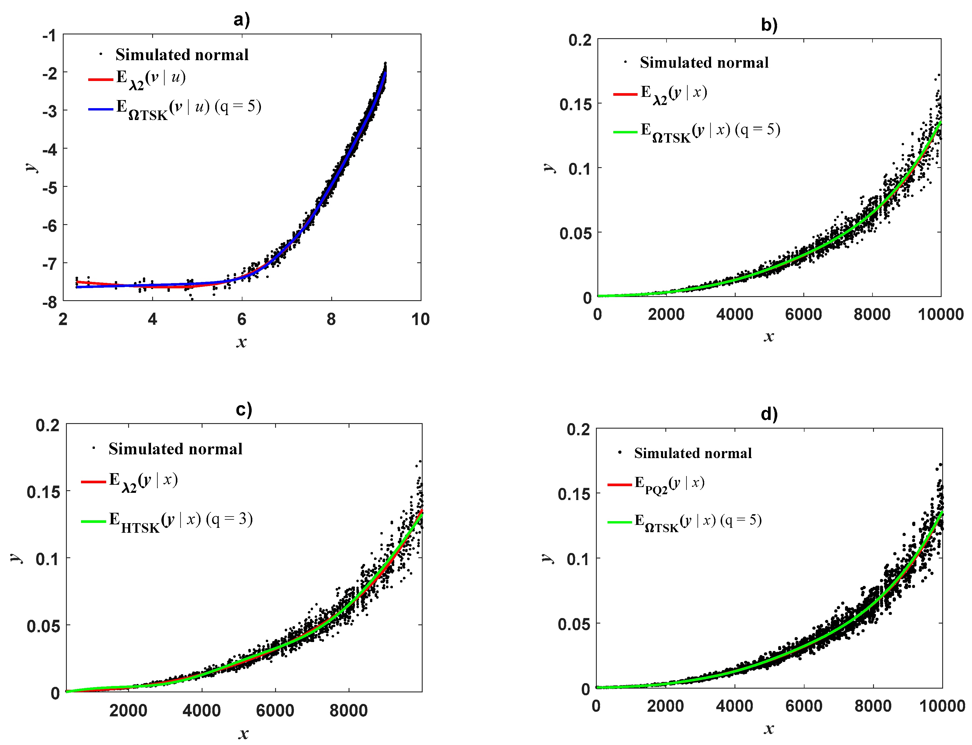
The results of Appendix E also reveal that a logarithmic transformation itself cannot be blamed for curvature detected in geometrical space. Simulation assays exhibit that geometrical space methods provide reliable proxies on condition that CF is chosen in a suitable form. 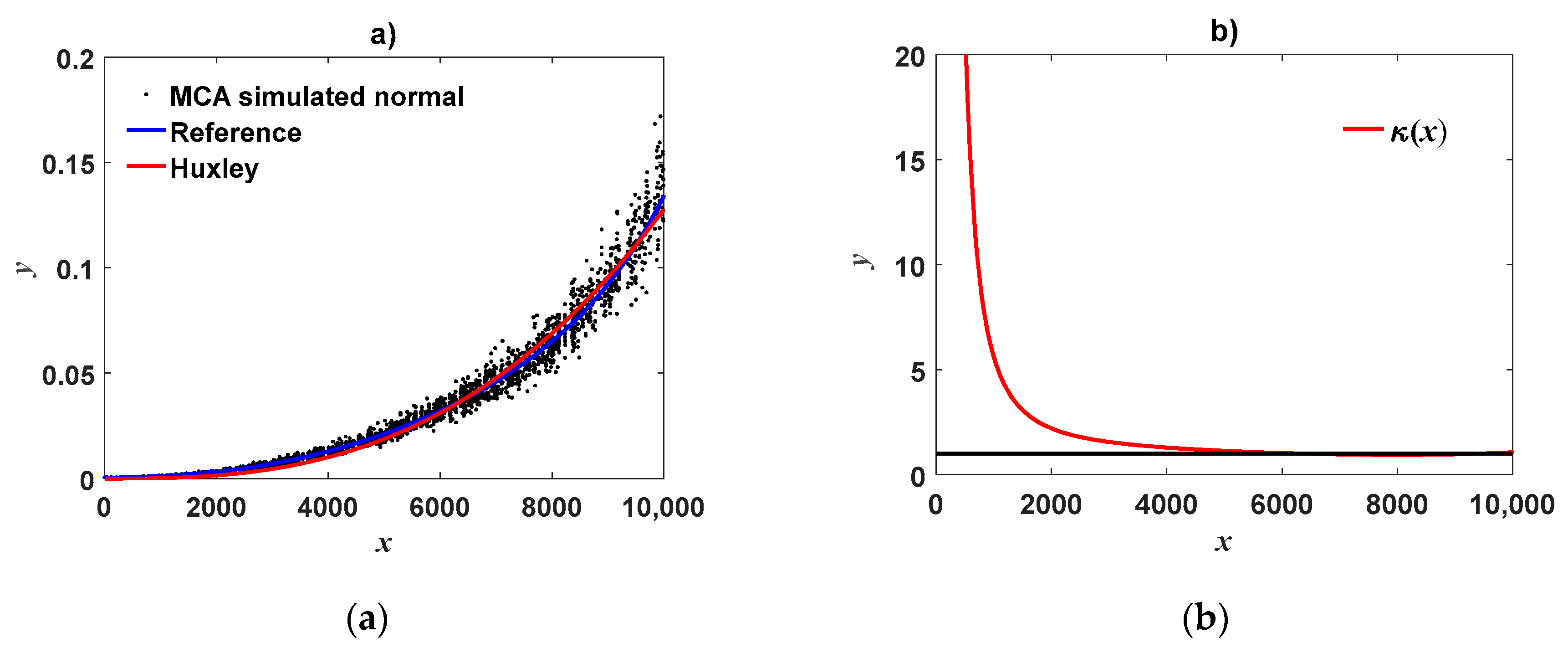However, the ${\lambda }_m\left(u\right)$ scheme could entail steady CF free retransformation to direct scales (Figure 3d and Figure 4d). This suggests that a suitable integration of complexity becomes a key factor in driving dependability of allometric projection based on protocols fitted on log-scales. Adoption of an ORBM approach also allowed adaptation of index κ(x) given by Equation (33) that interprets as a measure of curvature in geometrical space implied by the complexity of inherent allometric pattern in direct scales. Moreover, $\kappa \left(x\right)$ allows parallel criterion to statistical performance metrics for model selection. Results of simulation runs reveal that information based on $\kappa \left(x\right)$ can unravel efficiency of DNLR being only putative. Indeed, visual appraisal of a fit of Huxley’s model of simple allometry to simulated MCA replicates could suggest consistent reproducibility (Figure 1a). However, a concurrent plot of $\kappa \left(x\right)$ index (Figure 1b) exhibits noticeable deviations from the line $y=1$ for small values of the covariate. Similarly marked deviations of the $\kappa \left(x\right)$ from the line $y=1$ are shown in the biphasic fit to the Ramirez-Ramirez et al. [6] data (Figure 8d). Comparable effects are displayed for small eelgrass leaves (Figure 12d). This explains manifestation of curvature that was corroborated by dependability of the biphasic forms of the ${\Omega }_{TSK}\left(u\right), {\Omega }_{BL}\left(u\right)$ and ${\Omega }_{ML}\left(u\right)$ protocols. Therefore, clinging to Huxley’s model, and a non-linear regression protocol in direct scales can at most offer an apparent empirical convenience tied to simplicity, but it may leave behind relevant biological information. This concerns the existence of break points for transition between successive growth phases that are undetected by Huxley’s model of simple allometry and are well recognized by the PLA paradigm [91,93,94,95]. Likewise, identified break point in Zostera marina may perhaps be interpreted as a threshold beyond which the plant promotes generation of a relatively greater amount of tissue in leaves to enhance resistance to drag force effects that induce damage and separation from shoots. As a result, allometric scaling parameters among small and large leaves could be different [30]. Similarly, a break point in the Ramirez-Ramirez [6] data suggest differential allometric rules depending on tree size. Indeed, resource allocation to different tree attributes like diameter or height could differ during growth as a response to changed environmental-biotic conditions, as well as, to variations in resource availability. In this perception, a risk of suppression by competitors may induce small trees to dispense more resources to increase height. Then, beyond a threshold height at which suppression risk is at a minimum, resources may be assigned to horizontal growth parameters like diameter, crown and root cover [6,135]. Thus, since the aim of allometric examination is comprehending the biological processes that bring about covariance among traits, analytical methods entailing break point identification must be preferred. This explains adaptation of the empirical procedure of Appendix A aiming to extending the ${\lambda }_m\left(u\right)$ protocol for break point detection. In particular, the contemplated ${\Omega }_{TSK}\left(u\right)$ approach could be a highly biologically meaningful model of allometry, because it can model the break points while keeping the meanings of allometric exponents as Huxley’s original formulation. Moreover, as exemplified by the addressed study cases, the intersection of firing strength factors provides a reliable criterion to break point identification which could be expected to deliver reliable results in the general settings of allometric examination.

5. Conclusions

We aimed here to address the general identification problem of the MCA model of Equation (2). This conceived using regression protocols and data pairs $\left(x,y\right)$ in order to unfold $\alpha \left(x\right)$ and $\beta \left(x\right)$ as independent functions granting highest reproducibility. This task was addressed here in two ways. A first one was through Weierstrass approximation theory that anticipated $\alpha \left(x\right)$ and $\beta \left(x\right)$ as determined by Equation (8) through Equation (10) and that epitomize by the ${\lambda }_m\left(u\right)$ form in geometrical space. A second way to address the general identification problem relied on an ORBM slant. This conceived $\alpha \left(x\right)$ and $\beta \left(x\right)$ in the forms given by Equation (22) and Equation (23) respectively, and that engendered the ${\Omega }_{\mathit{B}\mathit{L}}\left(u\right)$, ${\Omega }_{ML}\left(u\right)$ and ${\Omega }_{TSK}\left(u\right)$ protocols also intended to be fitted in geometrical space. This ORBM approach is also behind the adaptation of the form $H_{TSK}\left(x\right)$ that takes advantage of the oustanding approximation capabilities of the general output of a first order TSK fuzzy model grants polyphasic interpolation of inherent MCA pattern in arithmetical scales.

A consistent fit of the ${\lambda }_m\left(u\right)$ arrangement could set up reliable reproducibility by direct retransformation to arithmetical scales. Moreover, this approach can also entail estimation of break point inherent to biphasic patterns. Concomitant broken line ${\Omega }_{BL}\left(u\right)$ or weighted linear segment mixture ${\Omega }_{ML}\left(u\right)$ regression could also offer reasonable MCA identification in many instances of allometric examination. Nevertheless, it is opportune to emphasize gains derived from adoption of a ${\Omega }_{TSK}\left(u\right)$ approach. This construct bears a flexible computational assembly that allows intuitive and interactive integration of previous knowledge into the analysis [132]. This gives ${\Omega }_{TSK}\left(u\right)$ a relative advantage over the conventional protocols addressed here. Moreover, analysis of model performance metrics show that the mean response function $E_{\Omega TSK}\left(y|\mathrm{x}\right)$ brings about similar reproducibility strength as its $E_{HTSK}\left(y|x\right)$ counterpart. Therefore, ${\Omega }_{TSK}\left(u\right)$ could grant efficient identification of allometric proxies indistinctly of inherent complexity. This device also drives direct and intuitive identification of multiple break points for transition among successive growth phases comprising a PLA pattern. It is also worth highlighting that the extraordinary approximation capabilities of a first-order KSK fuzzy model that engenders ${\Omega }_{TSK}\left(u\right)$ grant reliable identification of the scaling functions $\alpha \left(x\right)$ and $\beta \left(x\right)$ by retransforming fitted form of ${\Omega }_{TSK}\left(u\right)$ to arithmetical scales. We can then consider that the essential aim of this contribution was fulfilled. The TSK arrangement also allows efficient implementation of the $\kappa \left(x\right)$ criterion for curvature assessment. The identification schemes offered can be conveniently implemented on available data by using the codes provided. In summary, the presented MCA paradigm, along with identification schemes plus a suitable CF form could grant efficient projection of plant biomass units. This may well be also extended to the general settings of allometric examination. Nevertheless, we acknowledge that further substantiation is deemed necessary before proposed MCA could be adopted as a comprehensive tool for the analysis of allometric data. Meanwhile, present results endorse the relevance of the excerpt of Kerkhoff and Enquist [81] on the hopelessness of a divergence between traditional logarithmic transformation and direct non-linear analysis slants in allometry. Surely, the efficiency of the proposed MCA arrangement can elucidate this glowing controversy.

References

1. Litton, C.M.; Kauffman, J.B. Allometric Models for Predicting Aboveground Biomass in Two Widespread Woody Plants in Hawaii. Biotropica 2008, 40, 313–320. [Google Scholar] [CrossRef]
2. Alamgir, M.; Al-Amin, M. Allometric models to estimate biomass organic carbon stock in forest vegetation. J. For. Res. 2008, 19, 101–106. [Google Scholar] [CrossRef]
3. Gomes-de-Araujo, E.J.; Hambrecht-Loureiro, G.; Sanquetta, C.R.; Inoue-Sanquetta, M.N.; Dalla-Corte, A.P.; Péllico-Netto, S.; Behling-Floresta, A. Allometric models to biomass in restoration areas in the Atlantic rain forest. Floresta Ambient 2018, 25, 1–13. [Google Scholar]
4. Diédhiou, I.; Diallo, D.; Mbengue, A.; Hernandez, R.; Bayala, R.; Diémé, R.; Diédhiou, P.; Sène, A. Allometric Equations and Carbon Stocks in Tree Biomass of Jatropha Curcas L. in Senegal’s Peanut Basin. Glob. Ecol. Conserv. 2017, 9, 61–69. [Google Scholar]
5. Djomo, A.N.; Picard, N.; Fayolle, A.; Henry, M.; Ngomanda, A.; Ploton, P.; Mclellan, J.; Saborowski, J.; Adamou, I.; Lejeune, P. Tree Allometry for Estimation of Carbon Stocks in African Tropical Forests. Forestry 2016, 89, 446–455. [Google Scholar] [CrossRef]
6. Ramírez-Ramírez, G.; Avilés, L.R.Y.; Solorio-Sánchez, F.J.; Navarro-Alberto, J.A.; Dupuy-Rada, J.M. Shifts in Tree Allometry in a Tropical Dry Forest: Implications for above-Ground Biomass Estimation. Bot. Sci. 2019, 97, 167. [Google Scholar] [CrossRef]
7. Dube, T.; Onisimo, M.; Riyad, I. Quantifying aboveground biomass in African environments: A review of the trade-offs between sensor estimation accuracy and costs. Trop. Ecol. 2016, 57, 393–405. [Google Scholar]
8. Chen, L.; Ren, C.; Zhang, B.; Wang, Z.; Xi, Y. Estimation of Forest Above-Ground Biomass by Geographically Weighted Regression and Machine Learning with Sentinel Imagery. Forests 2018, 90, 582. [Google Scholar] [CrossRef]
9. Kumar, L.; Mutanga, O. Remote Sensing of Above-Ground Biomass. Remote Sens. 2017, 9, 935. [Google Scholar] [CrossRef]
10. Roy, P.S.; Ravan, S.A. Biomass Estimation Using Satellite Remote Sensing Data—An Investigation on Possible Approaches for Natural Forest. J. Biosci. 1996, 21, 535–561. [Google Scholar] [CrossRef]
11. Xu, Q.; Man, A.; Fredrickson, M.; Hou, Z.; Pitkänen, J.; Wing, B.; Ramirez, C.; Li, B.; Greenberg, J.A. Quantification of Uncertainty in Aboveground Biomass Estimates Derived from Small-Footprint Airborne LiDAR. Remote Sens. Environ. 2018, 216, 514–528. [Google Scholar] [CrossRef]
12. Baccini, A.; Goetz, S.J.; Walker, W.S.; Laporte, N.T.; Sun, M.; Sulla-Menashe, D.; Hackler, J.; Beck, P.S.A.; Dubayah, R.; Friedl, M.A.; et al. Estimated Carbon Dioxide Emissions from Tropical Deforestation Improved by Carbon-Density Maps. Nat. Clim. Chang. 2012, 2, 182–185. [Google Scholar] [CrossRef]
13. Marvin, D.C.; Asner, G.P.; Knapp, D.E.; Anderson, C.B.; Martin, R.E.; Sinca, F.; Tupayachi, R. Amazonian Landscapes and the Bias in Field Studies of Forest Structure and Biomass. Proc. Natl. Acad. Sci. USA 2014, 111, E5224–E5232. [Google Scholar] [CrossRef]
14. Zhu, X.; Liu, D. Improving Forest Aboveground Biomass Estimation Using Seasonal Landsat NDVI Time-Series. ISPRS J. Photogramm. Remote Sens. 2015, 102, 222–231. [Google Scholar] [CrossRef]
15. Kim, Y.; Yang, Z.; Cohen, W.B.; Pflugmacher, D.; Lauver, C.L.; Vankat, J.L. Distinguishing between Live and Dead Standing Tree Biomass on the North Rim of Grand Canyon National Park, USA Using Small-Footprint Lidar Data. Remote Sens. Environ. 2009, 113, 2499–2510. [Google Scholar] [CrossRef]
16. Elzein, T.M.; Blarquez, O.; Gauthier, O.; Carcaillet, C. Allometric equations for biomass assessment of subalpine dwarf shrubs. Alp. Bot. 2011, 121, 129. [Google Scholar]
17. Nordh, N. Above-Ground Biomass Assessments and First Cutting Cycle Production in Willow (Salix Sp.) Coppice—A Comparison between Destructive and Non-Destructive Methods. Biomass Bioenergy 2004, 27, 1–8. [Google Scholar] [CrossRef]
18. Lai, J.; Yang, B.; Lin, D.; Kerkhoff, A.J.; Ma, K. The Allometry of Coarse Root Biomass: Log-Transformed Linear Regression or Nonlinear Regression? PLoS ONE 2013, 8, e77007. [Google Scholar] [CrossRef]
19. Mascaro, J.; Litton, C.M.; Hughes, R.F.; Uowolo, A.; Schnitzer, S.A. Minimizing Bias in Biomass Allometry: Model Selection and Log-Transformation of Data. Biotropica 2011, 43, 649–653. [Google Scholar] [CrossRef]
20. Macfarlane, D.W.; Kuyah, S.; Mulia, R.; Dietz, J.; Muthuri, C.; Noordwijk, M.V. Evaluating a Non-Destructive Method for Calibrating Tree Biomass Equations Derived from Tree Branching Architecture. Trees 2014, 28, 807–817. [Google Scholar] [CrossRef]
21. Hamburg, S.P.; Homann, P.S. Utilization of Growth Parameters of Eelgrass, Zostera Marina, for Productivity Estimation under Laboratory and in Situ Conditions. Mar. Biol. 1986, 93, 299–303. [Google Scholar] [CrossRef]
22. Lu, M.; Caplan, J.S.; Bakker, J.D.; Langley, J.A.; Mozdzer, T.J.; Drake, B.G.; Megonigal, J.P. Allometry Data and Equations for Coastal Marsh Plants. Ecology 2016, 97, 3554. [Google Scholar] [CrossRef]
23. Cabrera, M.; Samboni-Guerrero, V.; Duivenvoorden, J.F. Non-destructive allometric estimates of above-ground and below-ground biomass of high-mountain vegetation in the Andes. Appl. Veg. Sci. 2018, 21, 477–487. [Google Scholar] [CrossRef]
24. Yandle, D.O.; Wiant, H.V., Jr. Estimation of Plant Biomass Based on the Allometric Equation. Can. J. For. Res. 1981, 11, 833–834. [Google Scholar] [CrossRef]
25. Savage, V.M.; Gillooly, J.F.; Woodruff, W.H.; West, G.B.; Allen, A.P.; Enquist, B.J.; Brown, J.H. The Predominance of Quarter-Power Scaling in Biology. Funct. Ecol. 2004, 18, 257–282. [Google Scholar] [CrossRef]
26. Packard, G.C.; Birchard, G.F. Traditional Allometric Analysis Fails to Provide a Valid Predictive Model for Mammalian Metabolic Rates. J. Exp. Biol. 2008, 211, 3581–3587. [Google Scholar] [CrossRef]
27. Hui, D.; Jackson, R.B. Uncertainty in Allometric Exponent Estimation: A Case Study in Scaling Metabolic Rate with Body Mass. J. Theor. Biol. 2007, 249, 168–177. [Google Scholar] [CrossRef]
28. Duncanson, L.; Rourke, O.; Dubayah, R. Small Sample Sizes Yield Biased Allometric Equations in Temperate Forests. Sci. Rep. 2015, 5, 17153. [Google Scholar] [CrossRef]
29. Mckechnie, A.E.; Wolf, B.O. The Allometry of Avian Basal Metabolic Rate: Good Predictions Need Good Data. Physiol. Biochem. Zool. 2004, 77, 502–521. [Google Scholar] [CrossRef]
30. Echavarría-Heras, H.; Leal-Ramírez, C.; Villa-Diharce, E.; Cazarez-Castro, N. On the Suitability of an Allometric Proxy for Nondestructive Estimation of Average Leaf Dry Weight in Eelgrass Shoots I: Sensitivity Analysis and Examination of the Influences of Data Quality, Analysis Method, and Sample Size on Precision. Theor. Biol. Med. Model. 2018, 15, 4. [Google Scholar] [CrossRef]
31. Echavarría-Heras, H.; Leal-Ramírez, C.; Villa-Diharce, E.; Cazarez-Castro, N.R. The Effect of Parameter Variability in the Allometric Projection of Leaf Growth Rates for Eelgrass (Zostera Marina L.) II: The Importance of Data Quality Control Procedures in Bias Reduction. Theor. Biol. Med. Model. 2015, 12, 30. [Google Scholar]
32. Solana-Arellano, E.; Echavarria-Heras, H.; Leal-Ramirez, C.; Lee, K.S. The Effect of Parameter Variability in the Allometric Projection of Leaf Growth Rates for Eelgrass (Zostera Marina L.). Lat. Am. J. Aquat. Res. 2014, 42, 1099–1108. [Google Scholar] [CrossRef]
33. Montesinos-López, A.; Villa-Diharce, E.; Echavarría-Heras, H.; Leal-Ramirez, C. Improved allometric proxies for eelgrass conservation. J. Coast. Conserv. 2018, 23, 71–91. [Google Scholar] [CrossRef]
34. Huxley, J. Problems of Relative Growth, by Sir Julian S. Huxley… With 105 Illustrations; Methuen: London, UK, 1932. [Google Scholar]
35. Myhrvold, N.P. Dinosaur Metabolism and the Allometry of Maximum Growth Rate. PLoS ONE 2016, 11, e0163205. [Google Scholar] [CrossRef] [PubMed]
36. West, G.B.; Brown, J.H. The Origin of Allometric Scaling Laws in Biology from Genomes to Ecosystems: Towards a Quantitative Unifying Theory of Biological Structure and Organization. J. Exp. Biol. 2005, 208, 1575–1592. [Google Scholar] [CrossRef]
37. Mayhew, T.M. Allometric Studies on Growth and Development of the Human Placenta: Growth of Tissue Compartments and Diffusive Conductances in Relation to Placental Volume and Fetal Mass. J. Anat. 2006, 208, 785–794. [Google Scholar] [CrossRef]
38. Paul, R.A.; Smyser, C.D.; Rogers, C.E.; English, I.; Wallendorf, M.; Alexopoulos, D.; Meyer, E.J.; Essen, D.C.V.; Neil, J.J.; Inder, T.E. An Allometric Scaling Relationship in the Brain of Preterm Infants. Ann. Clin. Transl. Neurol. 2014, 1, 933–937. [Google Scholar] [CrossRef]
39. Moore, B.R.; Page-Sharp, M.; Stoney, J.R.; Ilett, K.F.; Jago, J.D.; Batty, K.T. Pharmacokinetics, Pharmacodynamics, and Allometric Scaling of Chloroquine in a Murine Malaria Model. Antimicrob. Agents Chemother. 2011, 55, 3899–3907. [Google Scholar] [CrossRef] [Green Version]
40. Eleveld, D.J.; Proost, J.H.; Vereecke, H.; Absalom, A.R.; Olofsen, E.; Vuyk, J.; Struys, M.M.R.F. An Allometric Model of Remifentanil Pharmacokinetics and Pharmacodynamics. Anesthesiology 2017, 126, 1005–1018. [Google Scholar] [CrossRef]
41. Kwak, H.S.; Im, H.G.; Shim, E.B. A Model for Allometric Scaling of Mammalian Metabolism with Ambient Heat Loss. Integr. Med. Res. 2016, 5, 30–36. [Google Scholar] [CrossRef] [Green Version]
42. Champernowne, D. A model of income distribution. Econ. J. 1953, 63, 318–351. [Google Scholar] [CrossRef]
43. Samaniego, H.; Moses, M.E. Cities as Organisms: Allometric Scaling of Urban Road Networks. J. Transp. Land Use 2008, 1, 21–39. [Google Scholar] [CrossRef] [Green Version]
44. Li, X.; Wang, X.; Zhang, J.; Wu, L. Allometric Scaling, Size Distribution and Pattern Formation of Natural Cities. Palgrave Commun. 2015, 1, 15017. [Google Scholar] [CrossRef]
45. Coccia, M. New directions in measurement of economic growth, development and underdevelopment. J. Econ. Political Econ. 2017, 4, 383–395. [Google Scholar]
46. Coffey, W.J. Allometric growth in urban and regional social-economic systems. Can. J. Reg. Sci. 1979, 11, 49–65. [Google Scholar]
47. Neukum, G.; Ivanov, B.A. Hazards Due to Comets and Asteroids; University of Arizona Press: Tucson, AZ, USA, 1994; pp. 359–416. [Google Scholar]
48. Maritan, A. Network Allometry. Geophys. Res. Lett. 2002, 29. [Google Scholar] [CrossRef]
49. Liu, G.; Li, R.; he, J.; Li, W.; Lu, J.; Long, W.; Gao, P.; Cai, G.; Tang, M. Scaling relation of earthquake seismic data. Phys. A 2018, 492, 2092–2102. [Google Scholar] [CrossRef]
50. Wolinsky, M.A.; Edmonds, D.A.; Martin, J.; Paola, C. Delta Allometry: Growth Laws for River Deltas. Geophys. Res. Lett. 2010, 37. [Google Scholar] [CrossRef]
51. Bull, W.B. Allometric Change of Landforms. Geol. Soc. Am. Bull. 1975, 86, 1489. [Google Scholar] [CrossRef]
52. Zeng, W.S.; Tang, S.Z. Bias Correction in Logarithmic Regression and Comparison with Weighted Regression for Nonlinear Models. Nat. Preced. 2011, 24, 137–143. [Google Scholar] [CrossRef]
53. Robertis, A.D.; Williams, K. Weight-Length Relationships in Fisheries Studies: The Standard Allometric Model Should Be Applied with Caution. Trans. Am. Fish. Soc. 2008, 137, 707–719. [Google Scholar] [CrossRef]
54. Rodríguez, J.M.; Angón, E.; González, M.A.; Perea, J.; Barba, C.; García, A. Allometric Relationship and Growth Models of Juveniles of Cichlasoma Festae (Perciforme: Cichlidae), a Freshwater Species Native in Ecuador. Rev. de Biol. Trop. 2017, 65, 1185. [Google Scholar] [CrossRef] [Green Version]
55. Ofstad, E.G.; Herfindal, I.; Solberg, E.J.; Sæther, B.-E. Home Ranges, Habitat and Body Mass: Simple Correlates of Home Range Size in Ungulates. Proc. R. Soc. B Biol. Sci. 2016, 283, 20161234. [Google Scholar] [CrossRef] [PubMed]
56. Sutherland, G.D.; Harestad, A.S.; Price, K.; Lertzman, K. Scaling of Natal Dispersal Distances in Terrestrial Birds and Mammals. Conserv. Ecol. 2000, 4, 16. [Google Scholar] [CrossRef]
57. Eberhard, W.G. Static Allometry and Animal Genitalia. Evolution 2009, 63, 48–66. [Google Scholar] [CrossRef]
58. Houle, D.; Pélabon, C.; Wagner, G.P.; Hansen, T.F. Measurement and Meaning in Biology. Q. Rev. Biol. 2011, 86, 3–34. [Google Scholar] [CrossRef] [PubMed] [Green Version]
59. Pélabon, C.; Tidière, M.; Lemaître, J.-F.; Gaillard, J.-M. Modelling Allometry: Statistical and Biological Considerations—A Reply to Packard. Biol. J. Linn. Soc. 2018, 125, 664–671. [Google Scholar] [CrossRef]
60. Zar, J.H. Calculation and Miscalculation of the Allometric Equation as a Model in Biological Data. BioScience 1968, 18, 1118–1120. [Google Scholar] [CrossRef]
61. Smith, R.J. Logarithmic Transformation Bias in Allometry. Am. J. Phys. Anthropol. 1993, 90, 215–228. [Google Scholar] [CrossRef]
62. Hayes, J.P.; Shonkwiler, J.S. Allometry, Antilog Transformations, and the Perils of Prediction on the Original Scale. Physiol. Biochem. Zool. 2006, 79, 665–674. [Google Scholar] [CrossRef]
63. Packard, G.C.; Birchard, G.F.; Boardman, T.J. Fitting Statistical Models in Bivariate Allometry. Biol. Rev. 2011, 86, 549–563. [Google Scholar] [CrossRef] [PubMed]
64. Packard, G.C. Is Logarithmic Transformation Necessary in Allometry? Biol. J. Linn. Soc. 2013, 109, 476–486. [Google Scholar] [CrossRef] [Green Version]
65. Tausch, R.J.; Tueller, P.T. Comparison of regression methods for predicting single leaf pinyon phytomass. Great Basin Nat. 1988, 48, 39–45. [Google Scholar]
66. Packard, G.C. On the Use of Logarithmic Transformations in Allometric Analyses. J. Theor. Biol. 2009, 257, 515–518. [Google Scholar] [CrossRef]
67. Fattorini, S. To Fit or Not to Fit? A Poorly Fitting Procedure Produces Inconsistent Results When the Species–Area Relationship Is Used to Locate Hotspots. Biodivers. Conserv. 2007, 16, 2531–2538. [Google Scholar] [CrossRef]
68. Giosa, M.D.; Czerniejewski, P. A Generalized, Nonlinear Regression Approach to the Length-Weight Relationship of European Perch (Perca Fluviatilis L.) from the Polish Coast of the Southern Baltic Sea. Arch. Pol. Fish. 2016, 24, 169–175. [Google Scholar] [CrossRef] [Green Version]
69. Caruso, T.; Garlaschelli, D.; Bargagli, R.; Convey, P. Testing Metabolic Scaling Theory Using Intraspecific Allometries in Antarctic Microarthropods. Oikos 2010, 119, 935–945. [Google Scholar] [CrossRef] [Green Version]
70. Packard, G.C. Is Non-Loglinear Allometry a Statistical Artifact? Biol. J. Linn. Soc. 2012, 107, 764–773. [Google Scholar] [CrossRef] [Green Version]
71. Packard, G.C. On the Use of Log-Transformation versus Nonlinear Regression for Analyzing Biological Power Laws. Biol. J. Linn. Soc. 2014, 113, 1167–1178. [Google Scholar] [CrossRef] [Green Version]
72. Packard, G.C. The Essential Role for Graphs in Allometric Analysis. Biol. J. Linn. Soc. 2017, 120, 468–473. [Google Scholar] [CrossRef] [Green Version]
73. Mosimann, J.E. Size Allometry: Size and Shape Variables with Characterizations of the Lognormal and Generalized Gamma Distributions. J. Am. Stat. Assoc. 1970, 65, 930–945. [Google Scholar] [CrossRef]
74. Klingenberg, C.P. Size, Shape, and Form: Concepts of Allometry in Geometric Morphometrics. Dev. Genes Evol. 2016, 226, 113–137. [Google Scholar] [CrossRef] [PubMed]
75. Frankino, W.A.; Emlen, D.J.; Shingleton, A.W. Experimental Approaches to Studying the Evolution of Animal Form: The Shape of Things to Come. In Experimental Evolution Concepts, Methods, and Applications of Selection Experiments; California Scholarship Online: Berkeley, CA, USA, 2010; pp. 419–478. [Google Scholar]
76. Macleod, C. Exploring and Explaining Complex Allometric Relationships: A Case Study on Amniote Testes Mass Allometry. Systems 2014, 2, 379–392. [Google Scholar] [CrossRef] [Green Version]
77. Bervian, G.; Fontoura, N.F.; Haimovici, M. Statistical Model of Variable Allometric Growth: Otolith Growth in Micropogonias Furnieri(Actinopterygii, Sciaenidae). J. Fish Biol. 2006, 68, 196–208. [Google Scholar] [CrossRef]
78. Lovett, D.L.; Felder, D.L. Application of Regression Techniques to Studies of Relative Growth in Crustaceans. J. Crustacean Biol. 1989, 9, 529–539. [Google Scholar] [CrossRef]
79. Klingenberg, C.P. Heterochrony and Allometry: The Analysis of Evolutionary Change in Ontogeny. Biol. Rev. Camb. Philos. Soc. 1998, 73, 79–123. [Google Scholar] [CrossRef] [PubMed]
80. Nevill, A.M.; Bate, S.; Holder, R.L. Modeling Physiological and Anthropometric Variables Known to Vary with Body Size and Other Confounding Variables. Am. J. Phys. Anthropol. 2005, 128, 141–153. [Google Scholar] [CrossRef] [PubMed]
81. Kerkhoff, A.J.; Enquist, B.J. Multiplicative by Nature: Why Logarithmic Transformation Is Necessary in Allometry. J. Theor. Biol. 2009, 257, 519–521. [Google Scholar] [CrossRef]
82. Xiao, X.; White, E.P.; Hooten, M.B.; Durham, S.L. On the Use of Log-Transformation vs. Nonlinear Regression for Analyzing Biological Power Laws. Ecology 2011, 92, 1887–1894. [Google Scholar] [CrossRef] [Green Version]
83. White, E.P.; Xiao, X.; Isaac, N.J.B.; Sibly, R.M. Methodological Tools. Metab. Ecol. 2012, 1, 7–20. [Google Scholar]
84. Ballantyne, F. Evaluating Model Fit to Determine If Logarithmic Transformations Are Necessary in Allometry: A Comment on the Exchange between Packard (2009) and Kerkhoff and Enquist (2009). J. Theor. Biol. 2013, 317, 418–421. [Google Scholar] [CrossRef] [PubMed]
85. Glazier, D.S. Log-Transformation Is Useful for Examining Proportional Relationships in Allometric Scaling. J. Theor. Biol. 2013, 334, 200–203. [Google Scholar] [CrossRef] [PubMed]
86. Niklas, K.J.; Hammond, S.T. Assessing Scaling Relationships: Uses, Abuses, and Alternatives. Int. J. Plant Sci. 2014, 175, 754–763. [Google Scholar] [CrossRef]
87. Lemaître, J.F.; Vanpé, C.; Plard, F.; Pélabon, C.; Gaillard, J.M. Response to Packard: Make Sure We Do Not Throw out the Biological Baby with the Statistical Bath Water When Performing Allometric Analyses. Biol. Lett. 2015, 11. [Google Scholar] [CrossRef]
88. Mascaro, J.; Litton, C.M.; Hughes, R.F.; Uowolo, A.; Schnitzer, S.A. Is Logarithmic Transformation Necessary in Allometry? Ten, One-Hundred, One-Thousand-Times Yes. Biol. J. Linn. Soc. 2014, 111, 230–233. [Google Scholar] [CrossRef] [Green Version]
89. Huxley, J.S. Constant Differential Growth-Ratios and Their Significance. Nature 1924, 114, 895–896. [Google Scholar] [CrossRef]
90. Huxley, J.S. Further work on heterogonic growth. Biol. Zent. 1927, 47, 151–163. [Google Scholar]
91. Strauss, R.E.; Huxley, J.S. Problems of Relative Growth, new ed.; Johns Hopkins University Press: Baltimore, MD, USA, 1993. [Google Scholar]
92. Echavarría-Heras, H.; Leal-Ramírez, C.; Villa-Diharce, E.; Montesinos-López, A. Examination of the Effects of Curvature in Geometrical Space on Accuracy of Scaling Derived Projections of Plant Biomass Units: Applications to the Assessment of Average Leaf Biomass in Eelgrass Shoots. BioMed Res. Int. 2019, 2019, 3613679. [Google Scholar] [CrossRef]
93. Packard, G.C. Relative Growth by the Elongated Jaws of Gars: A Perspective on Polyphasic Loglinear Allometry. J. Exp. Zool. Part B Mol. Dev. Evol. 2016, 326, 168–175. [Google Scholar] [CrossRef]
94. Gerber, S.; Eble, G.J.; Neige, P. Allometric Space and Allometric Disparity: A Developmental Perspective in the Macroevolutionary Analysis of Morphological Disparity. Evolution 2008, 62, 1450–1457. [Google Scholar] [CrossRef]
95. Hartnoll, R. The Determination of Relative Growth in Crustacea. Crustaceana 1978, 34, 281–293. [Google Scholar] [CrossRef]
96. Heth, C.D.; Pierce, W.D.; Belke, T.W.; Hensch, S.A. The Effect of Logarithmic Transformation on Estimating the Parameters of the Generalized Matching Law. J. Exp. Anal. Behav. 1989, 52, 65–76. [Google Scholar] [CrossRef] [PubMed] [Green Version]
97. Mori, S.; Yamaji, K.; Ishida, A.; Prokushkin, S.G.; Masyagina, O.V.; Hagihara, A.; Hoque, A.T.M.R.; Suwa, R.; Osawa, A.; Nishizono, T.; et al. Mixed-Power Scaling of Whole-Plant Respiration from Seedlings to Giant Trees. Proc. Natl. Acad. Sci. USA 2010, 107, 1447–1451. [Google Scholar] [CrossRef] [PubMed] [Green Version]
98. Snelling, E.P.; Taggart, D.A.; Maloney, S.K.; Farrell, A.P.; Seymour, R.S. Biphasic Allometry of Cardiac Growth in the Developing KangarooMacropus Fuliginosus. Physiol. Biochem. Zool. 2015, 88, 216–225. [Google Scholar] [CrossRef] [PubMed]
99. Duffy, J.E. Ecology and Evolution of Eusociality in Sponge-Dwelling Shrimp. Evol. Ecol. Soc. Sex. Syst. 2007, 387–410. [Google Scholar]
100. Chave, J.; Andalo, C.; Brown, S.; Cairns, M.A.; Chambers, J.Q.; Eamus, D.; Fölster, H.; Fromard, F.; Higuchi, N.; Kira, T.; et al. Tree Allometry and Improved Estimation of Carbon Stocks and Balance in Tropical Forests. Oecologia 2005, 145, 87–99. [Google Scholar] [CrossRef]
101. Niklas, K. Size-Dependent Allometry of Tree Height, Diameter and Trunk-Taper. Ann. Bot. 1995, 75, 217–227. [Google Scholar] [CrossRef]
102. Niklas, K. Mechanical Properties of Black Locust (Robinia Pseudoacacia L.) Wood. Size- and Age-Dependent Variations in Sap- and Heartwood. Ann. Bot. 1997, 79, 265–272. [Google Scholar] [CrossRef] [Green Version]
103. Johansen, T.A.; Foss, B.A. Operating Regime Based Process Modeling and Identification. Comput. Chem. Eng. 1997, 21, 159–176. [Google Scholar] [CrossRef] [Green Version]
104. Johansen, T.A.; Foss, B.A. ORBIT—Operating Regime Based Modeling and Identification Toolkit. IFAC Proc. Vol. 1998, 30, 921–926. [Google Scholar] [CrossRef] [Green Version]
105. Baskerville, G.L. Use of Logarithmic Regression in the Estimation of Plant Biomass. Can. J. For. Res. 1972, 2, 49–53. [Google Scholar] [CrossRef]
106. Newman, M.C. Regression Analysis of Log-Transformed Data: Statistical Bias and Its Correction. Environ. Toxicol. Chem. 1993, 12, 1129–1133. [Google Scholar] [CrossRef]
107. Duan, N. Smearing Estimate: A Nonparametric Retransformation Method. J. Am. Stat. Assoc. 1983, 78, 605–610. [Google Scholar] [CrossRef]
108. Manning, W.G.; Newhouse, J.P.; Duan, N.; Keeler, E.B.; Leibowitz, A.; Marquis, M.S. Health insurance and the demand for medical care: Evidence from a randomized experiment. Am. Econ. Rev. 1987, 77, 251–277. [Google Scholar] [PubMed]
109. Koch, R.W.; Smillie, G.M. Comment on “River Loads Underestimated by Rating Curves” by R. I. Ferguson. Water Resour. Res. 1986, 22, 2121–2122. [Google Scholar] [CrossRef]
110. Manning, W.G. The Logged Dependent Variable, Heteroscedasticity, and the Retransformation Problem. J. Health Econ. 1998, 17, 283–295. [Google Scholar] [CrossRef]
111. Lin, L.I.-K. A Concordance Correlation Coefficient to Evaluate Reproducibility. Biometrics 1989, 45, 255. [Google Scholar] [CrossRef]
112. Brosowski, B.; Deutsch, F. An Elementary Proof of the Stone-Weierstrass Theorem. Proc. Am. Math. Soc. 1981, 81, 89–92. [Google Scholar] [CrossRef]
113. Faria, S.; Soromenho, G. Fitting Mixtures of Linear Regressions. J. Stat. Comput. Simul. 2010, 80, 201–225. [Google Scholar] [CrossRef]
114. Quandt, R.E.; Ramsey, J.B. Estimating Mixtures of Normal Distributions and Switching Regressions: Rejoinder. J. Am. Stat. Assoc. 1978, 73, 730–738. [Google Scholar] [CrossRef]
115. Muggeo, V.M.R. Segmented: An R Package to Fit Regression Models with Broken-Line Relationships. R News 2008, 8, 20–25. [Google Scholar]
116. Turner, T.R. Estimating the Propagation Rate of a Viral Infection of Potato Plants via Mixtures of Regressions. J. R. Stat. Soc. Ser. C (Appl. Stat.) 2000, 49, 371–384. [Google Scholar] [CrossRef]
117. Veaux, R.D.D. Mixtures of Linear Regressions. Comput. Stat. Data Anal. 1989, 8, 227–245. [Google Scholar] [CrossRef]
118. Viele, K.; Tong, B. Modeling with mixtures of linear regressions. Stat. Comput. 2002, 12, 315–330. [Google Scholar] [CrossRef]
119. Ding, C. Using regression mixture analysis in educational research. Pract. Assess. Res. Eval. 2006, 11, 1–11. [Google Scholar]
120. Takagi, T.; Sugeno, M. Fuzzy Identification of Systems and Its Applications to Modeling and Control. IEEE Trans. Syst. Manand Cybern. 1985, SMC-15, 116–132. [Google Scholar] [CrossRef]
121. Sugeno, M.; Kang, G. Structure Identification of Fuzzy Model. Fuzzy Sets Syst. 1988, 28, 15–33. [Google Scholar] [CrossRef]
122. Chiu, S.L. Fuzzy Model Identification Based on Cluster Estimation. J. Intell. Fuzzy Syst. 1994, 2, 267–278. [Google Scholar]
123. Castro, J.R.; Castillo, O.; Sanchez, M.A.; Mendoza, O.; Rodríguez-Diaz, A.; Melin, P. Method for Higher Order Polynomial Sugeno Fuzzy Inference Systems. Inf. Sci. 2016, 351, 76–89. [Google Scholar] [CrossRef]
124. Jang, J.S.; Sun, C.T.; Mizutani, E. Neuro-Fuzzy and Soft Computing: A Computational Approach to Learning and Machine Intelligence; Prentice-Hall: Upper Saddle River, NJ, USA, 1997. [Google Scholar]
125. Wang, L.-X.; Mendel, J. Fuzzy Basis Functions, Universal Approximation, and Orthogonal Least-Squares Learning. IEEE Trans. Neural Netw. 1992, 3, 807–814. [Google Scholar] [CrossRef]
126. McBride, G.B. A Proposal for Strength-of-Agreement Criteria for Lin’s Concordance Correlation Coefficient; National Institute of Water & Atmospheric Research: Hamilton, New Zeeland, 2005. [Google Scholar]
127. Gupta, H.V.; Sorooshian, S.; Yapo, P.O. Toward Improved Calibration of Hydrologic Models: Multiple and Noncommensurable Measures of Information. Water Resour. Res. 1998, 34, 751–763. [Google Scholar] [CrossRef]
128. Hauduc, H.; Neumann, M.B.; Muschalla, D.; Gamerith, V.; Gillot, S.; Vanrolleghem, P.A. Towards Quantitative Quality Criteria to Evaluate Simulation Results in Wastewater Treatment—A Critical Review. In Proceedings of the 8th Symposium on Systems Analysis and Integrated Assessment, St. Sebastian, Spain, 20 June 2011. [Google Scholar]
129. Zeng, W.; Duo, H.; Lei, X.; Chen, X.; Wang, X.; Pu, Y.; Zou, W. Individual Tree Biomass Equations and Growth Models Sensitive to Climate Variables for Larix Spp. in China. Eur. J. For. Res. 2017, 136, 233–249. [Google Scholar] [CrossRef]
130. Zeng, W.S.; Tang, S.Z. Goodness evaluation and precision analysis of tree biomass equations. Sci. Silvae Sin. 2011, 47, 106–113. [Google Scholar]
131. Martin, R.D.; Genoud, M.; Hemelrijk, C.K. Problems of allometric scaling analysis: Examples from mammalian reproductive Biology. J. Exp. Biol. 2005, 208, 1731–1747. [Google Scholar] [CrossRef] [PubMed] [Green Version]
132. Echavarria-Heras, H.; Castro-Rodriguez, J.R.; Leal-Ramirez, C.; Villa-Diharce, E. Assessment of a Takagi-Sugeno-Kang fuzzy model assembly for examination of polyphasic loglinear allometry. PeerJ 2019. Accepted. [Google Scholar]
133. Ying, H. General SISO Takagi-Sugeno Fuzzy Systems with Linear Rule Consequent Are Universal Approximators. IEEE Trans. Fuzzy Syst. 1998, 6, 582–587. [Google Scholar] [CrossRef]
134. Zeng, K.; Zhang, N.-Y.; Xu, W.-L. A Comparative Study on Sufficient Conditions for Takagi-Sugeno Fuzzy Systems as Universal Approximators. IEEE Trans. Fuzzy Syst. 2000, 8, 773–780. [Google Scholar]
135. Weiner, J. Allocation, Plasticity and Allometry in Plants. Perspect. Plant Ecol. Evol. Syst. 2004, 6, 207–215. [Google Scholar] [CrossRef]
136. Echavarría-Heras, H.; Leal-Ramírez, C.; Castro-Rodríguez, J.R.; Villa-Diharce, E.; Castillo, O. A Takagi-Sugeno-Kang Fuzzy Model Formalization of Eelgrass Leaf Biomass Allometry with Application to the Estimation of Average Biomass of Leaves in Shoots: Comparing the Reproducibility Strength of the Present Fuzzy and Related Crisp Proxies. In Fuzzy Logic Augmentation of Neural and Optimization Algorithms; Castillo, O., Melin, P., Kacprzyk, J., Eds.; Springer: Basel, Switzerland, 2018; pp. 329–362. [Google Scholar]
137. Parresol, B.R. Assessing tree and stand biomass: A review with examples and, critical comparisons. For. Sci. 1999, 45, 573–593. [Google Scholar]
138. Schlaegel, B.E. Testing, reporting, and using biomass estimation models. In Southern Forest Biomass Workshop; Gresham, C.A., Ed.; Belle W. Baruch Force Science Institute, Clemson University: Clemson, SC, USA, 1982; pp. 95–112. [Google Scholar]
139. Meyer, H.A. The standard error of estimate of tree volume from logarithmic volume equation. J. For. 1938, 36, 340–342. [Google Scholar]
Figure 1. Huxley’s model of simple allometry fitted on multiple-parameter complex allometry (MCA) data simulated based on a lognormal distribution Panel (a) displays spread of y k ( i ) ( ϵ ) replicates around the reference curve y = e x p ( P 2 ( x ) ) exp ( Q 2 ( x ) l n x ) compared to the fitted Huxley’s mean response. Panel (b) shows the plot of curvature index κ ( x ) . We can ascertain that deviations from linearity in geometrical space can be expected for this data.
Applsci 09 04965 g001
Figure 2. Fit of MCA on simulated data ( u i , v c k ( i ) ( ϵ ) ) . Regression Equation (46) was fitted to simulated ( u i , v k ( i ) ) data pairs. Panel (a) shows dispersion of v k ( i ) about the mean response function λ 2 ( u ) . This plot also shows the traditional analysis method of allometry’s (TAMA) fitted mean response λ 0 ( u ) . We can ascertain notorious bias by this last approach. Panel (b) shows corresponding retransformation results. Compared to significant reproducibility of mean response E λ 2 ( y | x ) TAMA’s counterpart E λ 0 ( y | x ) entails significant bias.
Applsci 09 04965 g002
Figure 3. Comparison of λ 2 ( u ) and Ω T S K ( u ) fits on lognormally distributed data. Panel (a) comparison of mean response functions fitted by means of a λ 2 ( u ) and a Ω T S K ( u ) proxies. Panel (b) compares related retransformed forms E λ 2 ( y | x ) and E Ω T S K ( y | x ) .   Panel (c) compares E λ 2 ( y | x )   to E H T S K ( y | x ) fitted by the regression model of Equation (33) in direct arithmetical scales. Panel (d) is a comparison of E Ω T S K ( y | x ) to E P Q 2 ( y | x ) , the directly acquired projection function. This can be obtained by replacing the fitted parameter vector P Q into addressed MCA form in arithmetical space. We can be aware of reliable projections even without a CF.By acquiring non lognormally distributed replicates y k ( i ) ( ξ ) = β exp ( α l n x i + ξ k ) according to procedure of Equation (44), we examined error structure effects on performance of addressed proxies. Figure 4 displays plots corresponding to retransformed forms. Table 2 presents related model performance statistics. Results reveal that reliability of the MCA and TSK approaches does not depend in error structure for the present assay.
Applsci 09 04965 g003
Figure 4. Comparison of λ 2 ( u ) and Ω T S K ( u ) MCA fits the simulated non-lognormally distributed data. Panel (a) comparison of mean response functions E λ 2 ( u | v ) and E Ω T S K ( u | v ) . Panel (b) compares related retransformed forms E λ 2 ( y | x ) and E Ω T S K ( y | x ) .   Panel (c) compares E λ 2 ( y | x ) to E H TSK ( y | x ) acquired from regression model of Equation (34) fitted in direct arithmetical scales. Panel (d) is a comparison of E Ω T S K ( y | x ) to E P Q 2 ( y | x ) , the directly acquired projection function. This is obtained by replacing fitted parameter vector P Q into addressed MCA form in arithmetical space. We can be aware of dependable projections even without a correction factor (CF).
Applsci 09 04965 g004
Figure 5. MCA proxies fitted in geometrical space for the Ramirez-Ramirez et al. [6] data. Panel (a) dispersion of response v about mean functions E λ 1 ( v | u ) . Panel (b) corresponding spreading about E Ω B L ( v | u ) . Panel (c) shows deviations of v values around polynomial mean response E π 3 ( v | u ) . Panel (d) shows scattering about E Ω M L ( v | u ) . The plots suggest consistency of MCA fits in all cases.
Applsci 09 04965 g005
Figure 6. Fit of the Ω TSK ( u ) proxy fitted for the Ramirez-Ramirez et al. [6] data. Panel (a) shows firing strengths ϑ 1 ( u ) and ϑ 2 ( u ) for the biphasic characterization ( q = 2 ) of Ω TSK ( u ) intersecting at break point. Panel (b) exhibits dispersion of v about fitted TSK mean response, vertical segment signposts estimated break point. Panel (c) shows residual dispersion about the zero line. Panel (d) displays normal QQ (quantile-quantile) plot.
Applsci 09 04965 g006
Figure 7. Plots of retransformed mean response functions identified for the Ramirez-Ramirez et al. [6] data. Panel (a) presents dispersion of observed values response values about mean response function E λ 1 ( y | x ) . Panel (b) displays corresponding spread about E Ω B L ( y | x ) . Panel (c) shows this around E π 3 ( y | x ) and panel (d) associates to named scattering about E Ω M L ( y | x ) panel (a), broken line Ω B L ( u ) (panel (b)), polynomial π 3 ( u ) (panel (c)) and mixture lines Ω ML ( u ) (panel (d)).
Applsci 09 04965 g007aApplsci 09 04965 g007b
Figure 8. Retransformed biphasic Ω T S K ( u ) (panel (a)), direct scales fitted biphasic H TSK ( x ) (panel (b)), Huxley’s model of simple allometry (panel (c)) and curvature index κ ( x ) (panel (d)). Deviations of fitted Huxley’s power function relative to E H T S K ( y | x ) in panel c) explain deviations of κ ( x ) from line y = 1 shown in panel (d).
Applsci 09 04965 g008
Figure 9. MCA protocols fitted in geometrical space for the Zostera marina data set. Panel (a) dispersion of response v about mean functions E λ 2 ( v | u ) . The break point signposted by vertical segment is determined by the interpolation lines criterion presented in Appendix A. Panel (b) shows corresponding spreading about E Ω B L ( v | u ) . Panel (c) shows deviations of v values around polynomial mean response E π 5 ( v | u ) . Panel (d) is for v spread about E M L ( v | u ) . Plots suggest consistency of MCA fits in all cases.
Applsci 09 04965 g009
Figure 10. Fit of the Ω T S K ( u ) proxy on the eelgrass data. Panel (a) shows firing strengths ϑ 1 ( u ) and ϑ 2 ( u ) for the biphasic characterization of Ω T S K ( u ) . Panel (b) exhibits dispersion of v about fitted TSK mean response E Ω T S K ( v | u ) vertical segment signposts estimated break point. Panel (c) shows residual dispersion about the zero line. Panel (d) displays normal QQ plot.
Applsci 09 04965 g010
Figure 11. Plots of retransformed MCA protocols fitted on logtransformmed eelgrass data. Panel (a) E λ 2 B I ( y | x ) function obtained by retransformation of interpolation lines E λ 2 B I ( v | u ) (Figure 9a) Panel (b) spread about E Ω B L ( y | x ) . Panel (c) presents dispersion around mean function E π 5 ( y | x ) produced by the π 5 ( u ) polynomial. Panel (d) displays spread about mean funcion E Ω M L ( y | x ) deriving from retransformation of the mixture lines proxy Ω M L ( u ) . These plots suggest remarkable consistency of the retransformed MCA output.
Applsci 09 04965 g011
Figure 12. Plots of retransformed Ω T S K ( u ) and direct H T S K ( x ) proxies identified on eelgrass data. Panel (a) shows spread about E Ω T S K ( y | x ) . Panel (b) depicts dispersion about fitted biphasic form H T S K ( x )   , ( q = 2 ) . Panel (c) compares H T S K ( x ) , ( q = 2 ) , to the power function by Huxley’s model of simple allometry fitted on direct scales. Panel (d) displays the plot of curvature index κ ( x ) . This plot exhibits curvature effects more pronounced for the smaller leaves.
Applsci 09 04965 g012