Abstract
With the advancement of robotics, the importance of service robots in society is increasing. It is crucial for service robots to understand their environment so that they can offer suitable responses to humans. To realize the use of space, robots primarily use an environment model. This paper is focused on the development of an environment model based on human behaviors. In this model, a new neural network structure called dynamic highway networks is applied to recognize humans’ behaviors. In addition, a two-dimensional pose estimator, Laban movement analysis, and the fuzzy integral are employed. With these methods, two new behavior-recognition algorithms are developed, and a method to record the relationship between behavior and environment is proposed. Based on the proposed environmental model, robots can identify abnormal behavior, provide an appropriate response and guide a person toward the desired normal behavior by identifying abnormal behavior. Simulations and experiments justify the proposed method with satisfactory results.
1. Introduction
With the rapid development of robots nowadays, service robots are becoming increasingly popular in ageing societies. It is necessary that such robots be capable of gathering information about their external environment. However, most robots are only able to consider physical information, such as images captured from cameras or depth information provided by a laser rangefinder. Given the wide variety of objects encountered in the environment, it is impossible to collect all possible appearances of objects to train robots to recognize them, regardless of whether the data are in the form of laser points or images. Therefore, it is necessary to develop a solution for this problem.
To extract extra information in the environment model, there are two principal methods: the semantic map and cognitive map. In the semantic map, semantic labels are recorded for the object in the environment so that the map can provide a semantic level of understanding of the environment. Nüchter and Hertzberg [1] defined this as “a map that contains, in addition to spatial information about the environment, assignments of mapped features to entities of known classes. Further knowledge about these entities, independent of the map contents, is available for reasoning in some knowledge base with an associated reasoning engine”. The semantic map focuses on tagging an object or area so that robots can understand the meaning of a statement and perform the appropriate action [2,3,4]. A cognitive map is a mentality model of a person to explain the mechanism of recording information from an environment. The cognitive map is constructed by the abstract information, such as landmarks, path and nodes [5].
Humans learn about an object and its function by imitating the interactions of other people with the object. Like animals can learn new behavior by observing other animals [6], people can gain benefit from imitating other people, and so do robots [7,8,9]. By learning the behavior that happens in a specific position, robots can understand the use of space. Therefore, recording human behavior in a specific position is the primary idea involved in creating a cognitive map.
In biology, a cognitive map is regarded as a cognitive representation of a specific location in space and is constructed from place cells, which are found in the hippocampus [10,11]. The activity of place cells in the cognitive map is associated with a specific location in the environment and the corresponding location is called the place field. Place cells provide the location in the environment in the same way as the global positioning system (GPS). The activity of place cells will be reset, called remapping, as seen in studies on rats in another environment. This explains the plasticity of the hippocampus and the rats’ ability to adapt. With the development of the brain, grid cells have been found in the entorhinal cortex [12]. The activity of a grid cell is associated not only with a specific location but with several locations in the environment. Grid cells provide an internal coordinate system for navigation. The cognitive map is formed of place cells and grid cells such that it memorizes and understands the use of space.
A lot of research that adapts the cognitive map to robot applications is focused on creating a mathematical model for navigation or building a map for navigation because the cognitive map tries to classify the mechanism of navigation and memory for the use of space [13,14]. There are some research works [15,16] that associate the use of space with behavior. However, the behavior of moving still remains unsolved, such as busy walking, idle walking, wandering and stopping [17].
However, the cognitive map is rarely recording the low-level human behavior in the map such as standing, sitting, picking up and object, waving a hand, etc. In [18], the authors proposed a behavior-based map which is divided into many sub-regions. For each region, all human movement directions are described as transition probabilities. This method described the relationship between human behaviors and the environment. Inspired by these articles, we devise a method to enable robots to understand an environment through human behavior not only on physical information alone. This method also records human behaviors in each cell of map and describes the human behaviors that are suitable for the specific location. Moreover, the proposed method can enable a robot to understand an environment automatically according to the behaviors of humans in that environment. To these ends, we focus on developing a behavior cognitive map that can recognize and record human behaviors. Robots based on this map can be used in diverse applications, for example, as exhibition assistants and patrol robots. In general, the task of creating a cognitive map can be divided into two steps: recognition of human behaviors and recording of human behaviors.
A system based on the proposed method can understand the use of space to enable robots to respond correctly to human behavior. The aforementioned behavior cognitive map that records the use of space by humans is designed based on two dimensions of human behavior models, namely the hand dimension and the body dimension. After fusing the behavioral features of humans, robots can identify whether a behavior is normal and provide an appropriate response. A block diagram of the structure of the proposed behavior cognitive map is shown in Figure 1. The aforementioned system has several functional components, including two-dimensional (2D) pose estimator using part affinity fields (PAFs), body behavior recognition using gated-recurrent-units (GRU)-based dynamic highway network (DHN), behavior-identification using Laban movement analysis, and behavior cognitive map. The first functional component is the 2D pose estimator using PAFs [19], which employs a convolutional neural network (CNN) and can draw a human skeleton on images. The second functional component, that is, the GRU-based DHN, is a combination of highway networks [20] and GRU neural networks [21]. The GRU-based DHN uses the skeleton position with the 2D pose estimator to predict body behavior. The third functional component is behavior identification. LMA [22,23] (Laban movement analysis) is applied to the skeleton positions to extract the features associated with hand behaviors. In LMA, 22 features are defined, and a similarity function is defined to calculate the similarity for the same behavior for each feature. Integrated similarity values estimated with the fuzzy integral algorithm [24]. Meanwhile, the positions of humans in images are estimated with simultaneous localization, mapping, and moving object tracking (SLAMMOT). Based on the estimated positions of humans, the normal behaviors recorded in the behavior cognitive map can be extracted and compared with observed behaviors.
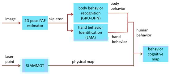
Figure 1.
Structure of a behavior cognitive map.
The remaining parts of this paper are organized as follows: Section 2 presents two modules for human behavior recognition and introduce the 2D pose estimator using PAFs and the GRU-based DHN. With these two functional components, a behavior-recognition model is constructed. In the behavior identification, the Laban movement analysis (LMA) is applied to identify the features that represent specific hand behaviors. The SLAMMOT is applied to construct the environment map. Section 3 introduces the behavior cognitive map. The interval recording method used in pedagogy is employed to record features into the behavior cognitive map. The similarity function and the fuzzy integral are applied to associate behaviors with specific positions. Identification of normal behaviors help robots react expediently. In Section 4, a series of simulations and experiments is presented and discussed. Finally, the results of the study are summarized in Section 5 and an outline for future work is given.
2. Human Behavior Recognition
Before building the cognition behavior map, the robot has to understand the human behavior. The first step is to establish a mechanism for recognizing human behavior. The task of human behavior recognition is divided into two parts: human pose estimation and behavior-recognition models. In 2D pose estimation, human postures are described with a skeleton. The information presented by the skeleton was used to train the two behavior-recognition models, namely, GRU-based DHN and similarity calculations of the Laban features.
2.1. 2D Pose Estimation
Cao at al. [19] proposed the 2D pose estimator using PAFs to address the human pose. The PAFs (part affinity fields) are the sets of 2D vector fields which describe the relation between human body joints. These vector fields can be used to extract the original position and location of each limb. This method retains the advantages of the heatmap and addresses several of its disadvantages. Thus, it will be used to estimate 2D poses from images.
A two-branch multi-stage CNN was used to calculate the PAFs and the joint confidence maps for each limb. The transformation function of the first branch of CNN, which is represented by ρ, is designed to predict the joint confidence maps. The set S = (S1, S2, …, SJ) contains J confidence maps, where denotes the confidence map of each body joint. The other branch’s transformation function of CNN, which is represented by φ, employs PAFs to express associations between joints. The set L = (L1, L2, …, LC) contains C vector fields, where denotes the 2D vector field in the relationship between body joints, also called limbs. In the first stage, the confidence maps and PAFs are represented as S1 = ρ1(F) and L1 = φ1(F). F is the output of a CNN initialized by the first 10 layers of VGG-19 [25]. Therefore, the 2D pose estimator using PAFs can be expressed as Equations (1) and (2):
where the superscript t denotes the variables at stage t. ρt and φt are the transformation function of CNN at the stage t. Finally, S and L follow the definitions given in the paragraph above.
To train the subnetworks ρ, it is necessary to generate the ground truth confidence map. The ground truth of confidence map satisfies the following equation:
where denotes any position on the confidence map; the ground truth position of the body joint j for person k; and σ the spread of joint j, which is set by the designer.
Instead of solving an integer linear programming problem, this method assembles body joints via 2D vector fields, called the PAFs. The PAFs are calculated by using CNNs, and they can consider large-scale features in an adjacent region. The PAF is a 2D vector field of each limb, and it preserves the position and orientation information. We formulate the ground truth of the PAF for training as (4):
where denotes any position on the PAF, the ground truth positions of body joints j1 and j2 for person k, and limb c the connection between and . To verify whether position x is on limb c, we define Equations (5) and (6). If position x satisfies Equations (5) and (6), then it is on limb c:
where x, and follow the definition in Equation (4), is a vector perpendicular to , and σl is a constant that controls the width of the vectors for each limb. Consequently, Equation (5) constrains the vectors that only exist between two joints, and Equation (6) constrains the vectors that exist at a specific distance from each other.
After training, the CNN can estimate a PAF that shows the possibility of association between two joints. Equations (7) and (8) are advanced to evaluate this probability:
where and denote the estimated positions of joints j1 and j2, respectively, and x(u) the interpolation of two joints. Using Equation (7), we can determine with certainty the relationship between two joints. After computing the relation of all joints, the human skeleton can be obtained. The axes of each joint, described as X, are collected as the inputs for two behavior-recognition models to identify the human behavior.
2.2. Body Behavior Recognition Model
The 2D pose estimator using PAF is useful for recognizing human behavior. Because human behavior is relative to time, the GRU (gated-recurrent-units) is necessary for learning temporal characteristics. Therefore, a new type of neural networks called GRU-based DHN is proposed.
Srivastava et al. [20] proposed highway networks based on the idea of bypassing a few upper layers and transmitting information to the deeper layers. In highway networks, a transform T(WTX+bT) is additionally defined to control the weights of the combination of input x and the output of the transform H(WHX+bH). However, the X is the axis of each joint from the human skeleton. The detailed function (Equation (9)) is illustrated in Figure 2:
where denote the input and output of a layer, respectively; the weights and bias in the transform T(WTX+bT); H an activation function, which is a rectified linear unit here; and T an activation function, which is a sigmoid function here. The dot operator denotes element-wise multiplication, and 1 denotes column vector with elements of 1.
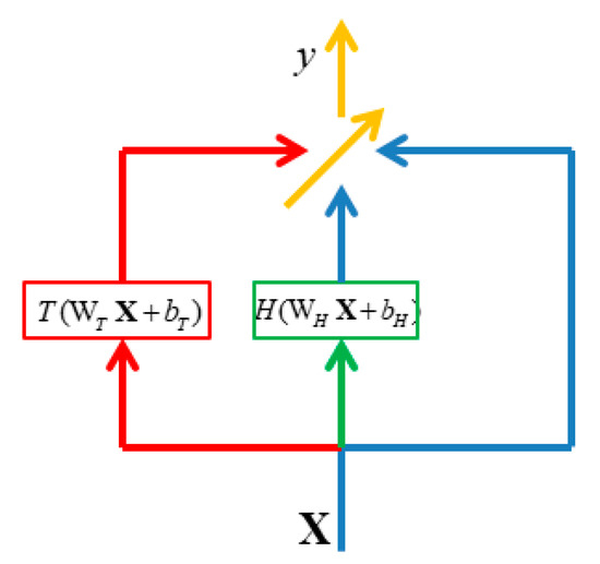
Figure 2.
Illustration of highway networks.
In addition, Equation (9) shows that y is a linear combination of input x and the output of the transform H(WHX+bH) in which the output of function T ranges between 0 and 1. Recalling the idea of the output of T(WTX+bT) the output denotes the weights of the combination of input x and the output of the transform H(WHX+bH) and backpropagation tunes the weights to minimize loss function. We can consider the weights to be tuned according to the utility of input and the output of the transform H(WHX+bH) through backpropagation.
Based on the idea of the output of T(WTX+bT) the utility of input x and the output of the transform H(WHX+bH) can be compared. The proposed dynamic high network (DHN) is expressed as Equations (10) and (11), and it is shown in Figure 3:
where denote the input, output, and middle input of the entire layer, respectively. denote the weights and the bias in the first and second layers, respectively, while H1, H2, T1, T2 are the activation functions. Here, X and y are called pass units, and d indicates growing units.
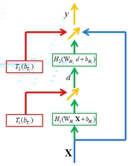
Figure 3.
Illustration of DHNs.
In DHNs, the function of the first layer is expressed as Equation (10). In this layer, compares the utility of ) with 0. Based on the values of , one can determine whether the number of neurons in the growing units is adequate. Consequently, the dimensionality of the growing units, n, can be raised until the values of are adequately small or the maximum permissible number of growing units is achieved. As a result, n can change dynamically according to the utility of ).
A GRU was proposed in [21]. The GRU is a structure of nodes. It is used in recurrent neural networks to learn the temporal features. The GRU introduces reset gates and update gates. Update gates avoid gradient diverging or gradient vanishing owing to the recurrent use of the same weights. The GRU is used instead of long short-term memory (LSTM) because the GRU model contains fewer parameters, which means the model can be trained faster and with lower memory usage. Information on human behavior is dependent on time. Therefore, extending the DHNs with the GRU model improves the behavior-recognition performance. The structure of the proposed GRU-based DHNs is illustrated in Figure 4.
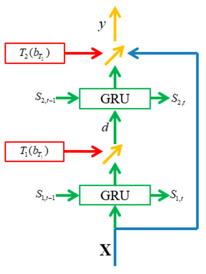
Figure 4.
Illustration of GRU-based DHNs.
In DHNs, the neurons are used as the normal nodes. There is no recurrent ability in the nodes, so they are unable to cope with temporal characteristics. In GRU-based DHNs, the neurons in the two sublayers are replaced with the GRU model to extend the model’s ability to address human behavior. Moreover, we use gates and in this model, with the same purpose as the forget gate in the LSTM model. This sublayer structure is intermediate between the GRU and the LSTM models.
As a result, the new model combining the 2D pose estimator using PAF and GRU-based DHNs is used to perform human skeleton estimation first, followed by behavior recognition, and it is shown in Figure 5. In other words, the 2D pose estimator using PAF first determines the 2D positions of the body joints; then, a GRU-based DHN is constructed to estimate human behavior from the movements of the body joints with time.
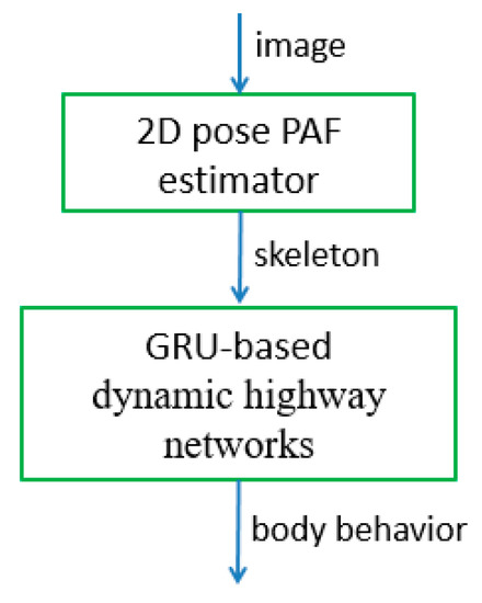
Figure 5.
Illustration of body behavior-recognition model.
2.3. Hand Behavior Identification Model
The human hand behavior is identified by using Laban movement analysis (LMA), which was proposed by Rudolf von Laban [22] to evaluate the similarity between the data and actual human action. This system combines psychology, anatomy, and kinesiology. It was developed for recording body language in dancing and has subsequently been widely used for behavior analysis. LAM not only records the positions of body joints but also describes the relationships among body representations, initial states, intentions, and emotions [26]. It divides human movement into the following elements: body, effort, shape, and space. These elements provide different aspects of information pertaining to human movement. In addition, they offer a few features to describe human movement, such as a dancer can adopt the correct pose for dancing based on the same foundation. Therefore, any dancer can recreate a masterpiece by using these basic elements, regardless of their cultural or language background.
The behavior of hands is represented by LMA. Laban movement analysis can be used to ascertain the principal information in a movement so that the movement can be identified easily based on the calculated LMA features. The 2D pose estimator using PAF estimates the skeletons of the people from a given image. With the skeleton information, the LMA features are extracted based on the description of the given LMA. These features are considered on the frontal plane because they only consist of 2D information and are normalized by shoulder width and height. Based on these features, the diverse behaviors of the hands can be recorded in the behavior cognitive map. The features used in each element are defined as follows:
- Body: The body feature describes the relationships between each limb while moving. We use nine distance features to describe the relationships and connections of each body joint. Therefore, we employ the distances from the hands to the shoulders, from the elbows to the shoulders, from the right hand to the left hand, from the hands to the head, and from the hands to the hips to represent the body.
- Effort: The effort features are used to understand the people’s inner intention, strength, timing, and control of movement. We use abrupt motions (jerky motion) of the hands and the hips as the features for the flow factor. We use acceleration of the hands as the feature for the weight factor. The time factors are extracted from the velocities of the hands. The above eight features are extracted as effort features.
- Shape: The shape describes the relationship between the body and environment. This research focuses on the hand’s behavior. So, we select three features to describe the shape features which are the height of both hands and the ratio of the distance from the hands to the center of the shoulder.
- Space: Space relates the motion and environment. It can be described as the space in which the human’s limbs can occupy. The area of the body can explain the relationship between the body and the environment. As a result, we use two area features, which are the area covered by the hands to the head and the hands to the hip, to indicate the space element.
We extract a total of 22 features, including nine distance features, two velocity features, two acceleration features, four jerk features, two position features, one distance ratio feature and two area features as the LMA features. These calculated features are recorded in the behavior cognitive map. Meanwhile, the behavior of the hand is predicted using the behavior-recognition model. The complete behavior-identification algorithm is illustrated in Figure 6.
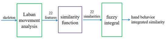
Figure 6.
Illustration of the hand behavior-identification algorithm.
A series of features is recorded, and these features are used to construct the corresponding vectors of the features that describe each behavior. The vector that contains the series of data for a specific feature f at time t is expressed as Vf(t). The vector that contains the series of data for a specific feature f and is recorded in the behavior cognitive map is expressed as . Therefore, the similarity between two behaviors for feature f can be calculated as the Euclidean distance between two vectors, as in Equations (12) and (13):
where the parameters of (13) are determined by trial and error.
The similarity value of the LMA features extracted from two similar hand behaviors is high. When the behavior resembles the recording behavior, the Euclidean distance is close to 0 and the similarity value is close to 1. Conversely, the similarity value is close to 0. After using Equation (13), the 22 similarity values of 22 features are obtained. In order to speed up the system and collect more gestures as possible, we use a fuzzy integral to fuse 22 features instead of using a model to identify what kind of behavior, and the fusing result is the final similarity value.
2.4. SLAMMOT (Simultaneous Localization, Mapping, and Moving Object Tracking)
The SLAMMOT [27,28] algorithm is widely used in mobile robotics so that robots are able to know their environment and also track moving objects. In this research, we use this method to track the moving objects by treating the participants who actively interact with one another in the area as the targeted moving objects. The SLAMMOT problem can be approximated as the posterior estimation, which can be shown as Equation (14):
where t is the time index, gt is the state of the robot, ot is the state of the moving object. Zt is observation, Ut is the control input. and denote measurements of stationary and moving objects, respectively. M is the environment map. It is used as a reference to record the location where the behavior arises from the body behavior model and hand behavior model. The detailed introduction to SLAMMOT, can be found in [8]. In the next section, the process of building the behavior cognitive map is carried out.
3. Behavior Cognitive Map
After recognizing human behavior, the next step is to record the behavior in the cognitive map in order to distinguish the normality of human motion. In biology, a cognitive map is regarded as a cognitive representation of a specific location in space, which is composed of place cells and grid cells, such that it memorizes and understands the use of space.
A cognitive map has been recognized as a mechanism for navigation and memory related to the use of space. Many robot applications [13,14] were focused on creating a mathematical model or building a navigation map. In the present study, we further develop the cognitive map and add records of human behavior to it to enhance the realization of the use of space. The proposed cognitive map, called a behavior cognitive map, establishes a relationship between a behavior and the location associated with the behavior. A few studies have associated the use of space with behavior. However, in those studies, the unclear motivation behaviors are related to states of movement, such as busy walking, idle walking, wandering, and stopping. In contrast, we introduce a variety types of behavior into the behavior cognitive map so that it can supply more information about the environment.
3.1. Recording Behavior
It is necessary to discuss the relevant human behaviors before creating the behavior cognitive map. In this study, we consider only those human behaviors that are associated with actions. The behaviors recorded in the behavior cognitive map should be daily or routine behaviors rather than unusual behaviors because the purpose of the behavior cognitive map is to learn the normal use of space. Thus, we collected datasets of daily behavior to determine representative daily behaviors.
Table 1 summarizes the contents of eight datasets: kth [29], IXMAS [30], MuHAVi [31], ACT4 [32], UCLA [33], HuDaAct [34], ASTS [35], and AIC [36]. We employ these datasets to determine the types of behavior that can be classified as representative daily behaviors based on the frequency of their occurrence, as highlighted in Table 1.

Table 1.
Behaviors in datasets.
The selected datasets contain only instances of low-level behaviors. High-level behaviors describe the interactions between a human and specific objects, i.e., behaviors that involve holding something and paying attention to it, such as a person using a smartphone or reading a book. The behavior cognitive map expresses the relationship between behavior and location, and records the use of space, it should describe how people tend to perform a specific behavior in a given location. Thus, the object of a person’s attention is not important for the behavior cognitive map, and such high-level behavior should be ignored. Moreover, it is impractical to consider such objects because a great number of them can be found in real environments. Therefore, we selected the datasets covering low-level behaviors as opposed to high-level behaviors.
As shown in Table 1, we choose seven representative daily highly repeated behaviors, namely, standing, walking, running, sitting, punching, hand waving, and picking up. In this study, we regard people as pedestrians if they are walking or running. Although the behavior cognitive map connects behavior with location, the behavior of pedestrians is not relative to their locations because they simply want to move toward their destination. For this reason, pedestrians are neglected in the behavior cognitive map. The remaining representative daily behaviors can be separated into two dimensions: the body and the hands. In the body dimension, standing, sitting, and picking up denote different body positions. In the hands dimension, punching and hand waving denote different hand positions.
This is illustrated in Figure 7.
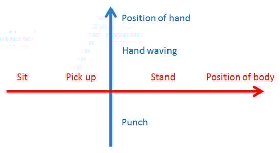
Figure 7.
Illustration of classic daily behaviors.
From the hand behaviors in Table 1, it is evident that the behaviors of the hands are not expressed adequately by punching and hand waving due to the great diversity of hand behaviors. To expand the behavior-recording capacity, hand behaviors are described with LMA in the behavior cognitive map. Unlike hand behaviors, body behaviors can be represented accurately by standing, picking up, and sitting. Therefore, the behavior-recognition model classifies the body behaviors as standing, picking up, and sitting. After this classification, the position information pertaining to these behaviors is recorded in the behavior cognitive map.
3.2. Structure of Behavior Cognitive Map
The behavior cognitive map is divided into three maps—sitting, picking up, and standing—because it is impossible for these three states to occur simultaneously. As one of these behaviors occurs, the behavior of the body is predicted, and the features of the behavior of the hands are calculated in accordance with the definition of body behaviors above. These features are recorded in the behavior map where the body is in the corresponding position. These maps are illustrated in Figure 8.
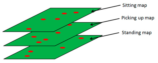
Figure 8.
Illustration of behavior cognitive map.
The red dots indicate that features are recorded at those locations. Thus, the behavior cognitive map is defined, and it can record the relationships between behaviors and the locations at which they occur. Therefore, a behavior can be decomposed into the body dimension and the hand dimension. In the body dimension, three body behaviors (standing, sitting, picking up) represent the body behavior. In the hand dimension, LMA is employed due to the large number of possible hand behaviors. The model structure is shown in Figure 9.
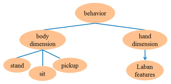
Figure 9.
Illustration of algorithms for behaviors in cognitive map.
In the behavior cognitive map, recording the frequency of behaviors is helpful for constructing a more ideal map. Based on the frequency of a behavior, a robot can determine whether that behavior is normal or not. Therefore, the behavior cognitive map can learn online and revise itself to adjust to dynamic environments.
Many methods have been proposed to record behavior, such as continuous recording, duration recording, time sampling, and interval recording. Of these methods, interval recording is suitable for our purpose and has been employed in the proposed behavior cognitive map. Interval recording records the occurrence of a given behavior in specified periods. The total observation time is divided into smaller intervals. Therefore, the total observation time should be decided first. According to the AVA dataset [37], an observation period of 1 s is adequate to recognize a behavior. Thus, we selected this observation period. The number of intervals is determined by the processing time of the program. In each interval, each feature is calculated and recorded.
3.3. Behavior Identification
To clarify the use of space, comparing the behavior in the behavior cognitive map and the behavior of a person at a given moment is an essential function of robots. A robot that can judge whether a behavior is normal can help a person to complete a task or prevent a person from completing a prohibited task.
In the behavior cognitive map, we have not selected specific behaviors as classifiers because it is impossible to classify all possible behaviors through the integration of all possible features and infer the results. Therefore, we have employed a similarity function to estimate similarities and integrated these similarities by using a fusion algorithm. From the final similarity, hand behaviors are identified as being either distinct or not distinct. To this end, we have applied a fusion algorithm called fuzzy integral to compute the extent of the similarity between hand behavior database and online testing data based on the features proposed. Sugeno introduced a non-additive “fuzzy” measure by replacing the additive property with the weaker monotonicity property [24], based on which the fuzzy integral was proposed. The fuzzy integral combines information from different sensors according to a non-linear function based on a fuzzy measure. Because of the concept of the fuzzy measure, the fuzzy integral has been widely applied. The principles of the fuzzy measure and fuzzy integral are introduced as Equation (15):
where r(ε) denotes the final similarity of all features. ε is the set for each measure feature that is represented as ε = {ε1, ε2, …, ε22}. ∨ and ∧ denote the maximum operator and minimum operator. h(mi) is the measure result for model mi. There are 22 models which use the thresholds to classifier the feature is similar or not. The finite set is defined as and a subset and g is a -fuzzy measure, the value of g(Ai) can be determined as:
and the λ value can be calculated by Equation (18):
In this research, we use F-score defined gi to perform the fuzzy integral operations. After computing the λ value, the final similarity can be obtained.
An F-score set is created to express the reliability of each model for a positive class. In the F-score set, each F-score serves as a measure to judge the evaluation of a model. Two parts are considered for calculating the F-score—precision p and recall r. The precision p expresses the proportion of correct estimates of a positive result among all positive estimations. The recall r expresses the proportion of correct estimates of a positive result among all correct estimations. The detailed calculation is shown in Figure 10.
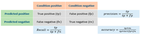
Figure 10.
Classification context.
The F-score can be regarded as a weighted average of the precision and the recall for evaluating the performance of a model. The precision, recall, and F-score are related as follows:
The behaviors of the body can be represented by standing, picking up, and sitting. In relative terms, the behaviors of the hands are too wide-ranged, which makes it difficult to select representative behaviors. Therefore, the behaviors of the hands are described with LMA. Laban movement analysis defines 22 features, and these features are adequate to represent the behaviors of the hands. As a result, these features are recorded in the behavior cognitive map at the corresponding positions. With these features, the similarity of each feature can be calculated between two behaviors. The fuzzy integral is then introduced to integrate all features. Thereafter, the final similarity between two behaviors can be calculated. Consequently, a robot can determine whether a behavior is normal and select the correct response to interact with a person.
4. Experimental Results
4.1. Human Behavior Recognition Experiments
We used a camera to capture images of humans, from which skeletons were extracted. This camera was capable of capturing images at the rate of 5 frames per second with a resolution of 640 × 480 pixels. The height of the camera was 80 cm, which is suitable for capturing the human body. The distance between the camera and the human was set to approximately 260 cm.
Data were collected from six participants. Moreover, to enrich the dataset, we scaled down and randomly shifted the original data. The details of the resulting dataset are presented in Table 2. The three-fold cross validation method was used to validate the proposed behavior-recognition model.
Table 2.
Behavior in datasets.
Because GRU-based DHNs need a data sequence, we must truncate serial data. According to the interval recording method, the truncated size is 5 frames. The sliding window algorithm was employed to perform data preprocessing for the GRU model. The sliding window was shifted one sample each time to reserve as much data as possible. To ensure the superiority of GRU-based DHNs over DHNs in terms of behavior recognition, we created a GRU-based DHN and a DHN with 10 layers and 128 neurons in each layer.
The test results are shown in Figure 11 and summarized in Table 3. In Figure 11, DHN denotes DHNs and GRU-DHN denotes GRU-based DHNs. The GRU-based DHNs exhibit superior behavior-recognition performance, with accuracy exceeding 99.5%.
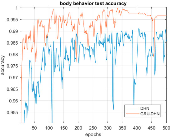
Figure 11.
Test results obtained with the behavior-recognition model.
Table 3.
Confusion matrix of GRU-based DHN.
Figure 11 shows the training process. With the increase of training epoch, GRU-based DHNs has maintained better performance than DHNs in most cases until the training process is completed. It proves that the temporal property must be considered to recognize the human behavior. The accuracy of GRU-based DHNs is higher than DHNs because they use a greater quantity of features (temporal property).
The following series of figures show the results of online continuous testing, which illustrate this inference. Figure 12 shows continuous frames extracting from a video and each panel shows three sub-images (Figure 12; see the video for Supplementary Materials S1, https://youtu.be/oHLd-O9n_Og). For each panel, the top sub-image shows the original image captured using the camera. The bottom-left sub-image shows the skeleton predicted by the DHN. The bottom-right sub-image shows the skeleton predicted by the GRU-based DHN. For example, in Figure 12a, the original image shows the participant stands. The predictions of body posture for two different classifiers are stand. It shows that both classifiers can be recognized correctly. Figure 12b,c,e also show the same situation. However, some moments indicate distinct situations.
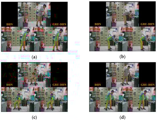
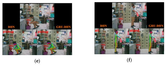
Figure 12.
Online continuous testing of the behavior-recognition model. (a) Stand motion at 23 s (b) Pick up motion at 33 s (c) Sit motion at 40 s (d) Stand motion with different prediction result at 57.5 s (e) Pick up motion at 78 s (f) Stand motion with different prediction result at 85.5 s (sec).
In Figure 12d,f, the original images show obviously the participant stand, and the GRU-DHN recognizes correct prediction as stand, but the DHN recognizes the wrong result as sit. The above results show that the temporal characteristics contribute to the identification of body movements. For this reason, GRU-based DHN can effectively improve classification performance. As a result, the GRU-based DHNs are selected to recognize body postures.
4.2. Experiments Involving Abnormal Behaviors
In order to fuse the similarities of the features by using the fuzzy integral algorithm, the reliability of each similarity is necessary. The reliability of each similarity was calculated in terms of the F-score. From Table 1, five representative hand behaviors, namely, hand waving, throwing, eating, punching, and making a phone call, were selected. To calculate the F-score and the accuracy of each feature, a threshold was set for each feature. If the calculated similarity was greater than the corresponding threshold, the two behaviors were regarded as the same behavior for the feature in question.
The λ value in the λ-fuzzy measure theory of the Sugeno fuzzy integral can be calculated. The λ value is shown as follows:
After obtaining the λ value, the Sugeno fuzzy integral can be calculated, and the prediction result can be obtained from the classification of the fuzzy integral.
The numbers in Table 4 shows how many data are classified as learnt behaviors. For example, the first column shows the numbers of each behavior recognized as hand waving. From the results in Table 4, the accuracy is 84.98%.
Table 4.
Confusion matrix of GRU-based DHN.
The behavior cognitive map is constructed with many blocks. Each block represents an area measuring 30 cm × 30 cm in the real world, and the behaviors occurring in this area are recorded in the same block. In this experiment, the robot constructs behavior cognitive map for an exhibition. The size of the room used in experiments is 700 cm × 700 cm. Figure 13 shows the physical map obtained with laser points and the behavior cognitive map. The physical map is shown in Figure 13a. The physical map only records the spatial relation to locate the robot, static objects, and participants. The red points represent the static objects, and the blank space represents the space people can walk. According to the physical map, the robot can only know the range of the visitors’ activities.
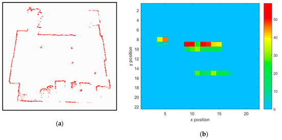
Figure 13.
Comparison of physical map and behavior cognitive map. (a) Physical map (b) Behavior cognitive map.
Figure 13b shows an example of the behavior cognitive map in which each grid represents the number of occurrences of human behavior. Because the behavior cognitive map records the features of behaviors directly, it can only show the number of features in each block to illustrate the use of space. The color bar represents the number of times of the behavior has occurred. Red means more times and blue means no behavior appeared. From the recorded behavior cognitive map, people tend to stand in front of tables and perform some behaviors when they visit the exhibition. In the exhibition room, there are guidebooks on a small table at the location (5.8) and some posters at the locations (8, 9) to (15, 9) and (10, 14) to (17, 14). The following human behavior is collected: People read books in front of a small table at the location (5, 8) and enjoy exhibitions from the locations (8, 11) to (15, 11) and from the locations (10, 15) to (17, 15). Clearly, the red color denotes the space where people visit most frequently, and the blue color denotes the space where the robot does not record any behavior. The behavior cognitive map indicates that visitors keep a distance from the posters to appreciate the exhibitions. So, the behavior recording locations are different from the poster location. However, the guidebooks are taken directly, so the reading behavior is recorded at the same location.
From the behavior cognitive map, we can determine the frequency of each behavior. A frequency threshold was defined to determine whether a behavior is normal. This threshold was calculated as the ratio of the number of records of a specific behavior to the total number of records. In real-time abnormal behavior recognition, we divided the number of records of specific behavior by the total number of records and compared this frequency ratio with the threshold to determine whether it was the abnormal behavior or not. Moreover, we defined a response threshold in the behavior cognitive map to judge whether a robot should respond and accumulate variables for each block in each block of the behavior cognitive map. If any value at any position in the map reaches the threshold, the robot should approach the human and offer the corresponding response. If some abnormal behaviors happen, the robot goes to stop the behavior and then goes back to the original position.
4.3. Summary
The aforementioned experiments attempted to demonstrate the abilities of the behavior-recognition model, behavior identification, and behavior cognitive map respectively. To demonstrate the implementations of the human–robot interaction, we conducted an experiment involving a robot providing a guided tour of our laboratory to human visitors by using the behavior cognitive map proposed herein. The mobile robot, called Bunny, is constructed by our laboratory. Bunny is equipped with a LMS-291 laser range finder (SICK, Waldkirch, Germany) with 180 degrees’ visibility range used for location and path planning purposes. It is equipped with sonar sensors and four camera sensors and a Kinect depth camera sensor (Microsoft, Redmond, Washington, USA). Beside its high performance main computer, Bunny also has an on-board Jetson TX2 module NVIDIA (Santa Clara, California, USA). In our case, the TX2 module is responsible for highly computationally complex tasks requiring parallel computing. Figure 14 shows a scenario in which some visitors obstruct the tour path. (Figure 14; see Supplementary Materials video for S2, https://youtu.be/zdXxsIIVGR8).
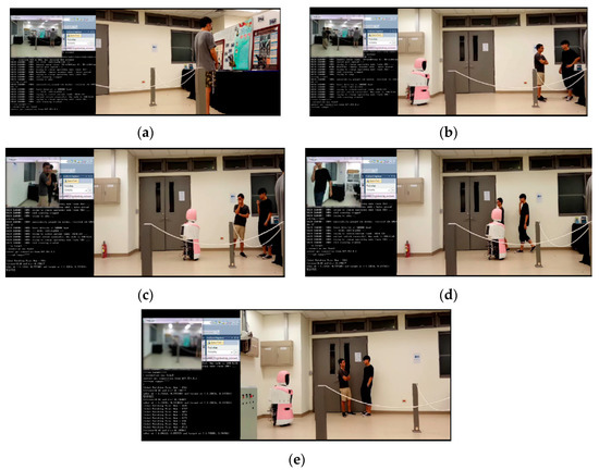
Figure 14.
Scenario of some visitors obstructing the tour path (a) A visitor looks the exhibit at 4 s (b) Two visitors obstruct the path at 13 s. (c) Bunny detects the abnormal behavior and asks two visitors to leave at 26 s. (d) Two visitors move to other location at 32 s. (e) Bunny goes back the original position at 70 s (sec).
Figure 14a shows that the robot recognizes the normal behavior of the person in the gray T-shirt and does not offer any response. However, Figure 14b shows two people obstructing the tour path. Immediately, the robot figured out that people tend to not stand in this location. Therefore, the robot approached them and suggested that they should not stand in that location, as shown in in Figure 14c,d. After they left the position, the robot returned to its original position and waited for the next contingency.
5. Conclusions
In this paper we have proposed a behavior cognitive map that can help mobile service robots understand the use of space. Using the proposed behavior cognitive map, robots can recognize normal and abnormal behaviors at specific locations in the environment. To construct the behavior-recognition model, we combined the 2D pose estimator using PAF and GRU-based DHNs to create a behavior-recognition model that can recognize postures of the human body. We then proposed a behavior-identification algorithm to determine whether the behaviors of two hands are identical. Multi-feature fusion, which can dynamically balance the result based on objective predictions and the importance or reliability of the features, was realized through Sugeno fuzzy integral fusion. These behaviors were recorded on the behavior cognitive map directly based on the location of their occurrence. Therefore, the use of space was realized, and any abnormal behavior can be identified by the proposed system. Finally, the aforementioned behavior-recognition system and the behavior cognitive map were implemented on a mobile robot, and behavior-recognition and servicing experiments were conducted. The results of the experiments showed that the robot can easily identify abnormal behavior and provide appropriate responses in human–robot interaction tasks.
The behavior cognitive map is used to build the human behaviors. This method complements the cognitive map without considering low-level human behaviors. This model lets the robot know what kinds of human behaviors usually occur at the specific space. However, this method does not consider the situation that the surrounding environment may change. For instance, the exhibitions are moved to other locations and the visiting traffic flow is changed. These situations will invalidate the behavior cognitive map.
In future work, there are three aspects in our research. First, add objects in the environment to the behavior cognitive map. It may help the cognitive map more complete and provide the ability to identify the abnormal behaviors that human interact with objects. Furthermore, it protects human to avoid the dangerous or inappropriate situation. Second, add adaptive functions. The behavior cognitive map can be adjusted as the spatial relationship changes. Finally, our approach will be extended to record high-level behaviors. Based on this extension, the robot can recognize more complex human behaviors.
Supplementary Materials
The following are available online at https://www.mdpi.com/2076-3417/9/23/5026/s1. There are two supplementary videos. The video S1 is the full video showing the online continuous testing experiment of the behavior-recognition model. Video S2 is the full video about the cognitive behavior map experiment—scenario of some visitors obstructing the tour path.
Author Contributions
Conceptualization, W.-Z.L., S.-H.W., and H.-P.H.; methodology, W.-Z.L., S.-H.W., and H.-P.H.; software, W.-Z.L. and S.-H.W.; validation, W.-Z.L. and S.-H.W.; formal analysis, W.-Z.L. and S.-H.W.; investigation, W.-Z.L., S.-H.W., and H.-P.H.; resources, W.-Z.L., S.-H.W., and H.-P.H.; data curation, W.-Z.L. and S.-H.W.; writing—original draft preparation, W.-Z.L. and S.-H.W.; writing—review and editing, W.-Z.L., S.-H.W. and H.-P.H.; visualization, W.-Z.L., S.-H.W. and H.-P.H.; supervision, H.-P.H.; project administration, H.-P.H.; funding acquisition, H.-P.H.
Funding
This research received no external funding.
Conflicts of Interest
The authors declare no conflict of interest.
References
- Nüchter, A.; Hertzberg, J. Towards Semantic Maps for Mobile Robots, Robotics and Autonomous System. Robot. Auton. Syst. 2008, 56, 915–926. [Google Scholar] [CrossRef]
- Liu, Z.; Wang, W. A Coherent Semantic Mapping System based on Parametric Environment Abstraction and 3D Object Localization. In Proceedings of the European Conference on Mobile Robots, Barcelona, Spain, 25–27 September 2013; pp. 234–239. [Google Scholar] [CrossRef]
- Rusu, R.B.; Marton, Z.C.; Blodow, N.; Holzbach, A.; Beetz, M. Model-based and Learned Semantic Object Labeling in 3D Point Cloud Maps of Kitchen Environments. In Proceedings of the IEEE/RSJ International Conference on Intelligent Robots and Systems, St. Louis, MO, USA, 10–15 October 2009; pp. 3601–3608. [Google Scholar] [CrossRef]
- Zhou, H.; Jiang, M. Building a Grid-point Cloud-semantic Map based on Graph for the Navigation of Intelligent Wheelchair. In Proceedings of the 21st International Conference on Automation and Computing (ICAC), Glasgow, UK, 11–12 September 2015; pp. 267–274. [Google Scholar] [CrossRef]
- Kitchin, R. Cognitive maps. In International Encyclopedia of the Social & Behavioral Sciences; Smelser, N., Baltes, P., Eds.; Elsevier: Pergamon, Turkey; Oxford, UK, 2001; pp. 2120–2124. [Google Scholar] [CrossRef]
- Rizzolatti, G.; Craighero, L. The mirror-neuron system. Annu. Rev. Neurosci. 2004, 27, 169–192. [Google Scholar] [CrossRef] [PubMed]
- Gaussier, P.; Moga, S.; Banquet, J.P.; Quoy, M. From Perception-action Loop to Imitation Processes: A Bottom-up Approach of Learning by Imitation. Appl. Artif. Intell. 1998, 12, 701–727. [Google Scholar] [CrossRef]
- Lagarde, M.; Andry, P.; Gaussier, P.; Boucenna, S.; Hafemeister, L. Proprioception and Imitation: On the Road to Agent Individuation. Stud. Comput. Intell. 2010, 264, 43–63. [Google Scholar]
- Laroque, P.; Gaussier, N.; Cuperlier, N.; Quoy, M.; Gaussier, P. Cognitive map plasticity and imitation strategies to improve individual and social behaviors of autonomous agents. Paladyn J. Behav. Robot. 2010, 1, 25–36. [Google Scholar] [CrossRef]
- O’Keefe, L.N.J. The Hippocampus as a Cognitive Map; Oxford University: Oxford, UK, 1987. [Google Scholar]
- O’Keefe, J.; Conway, D.H. Hippocampal Place Units in the Freely Moving Rat: Why They Fire Where They Fire. Exp. Brain Res. 1978, 31, 573–590. [Google Scholar] [CrossRef] [PubMed]
- Sargolini, F. Conjunctive Representation of Position, Direction, and Velocity in Entorhinal Cortex. Science 2006, 312, 758–762. [Google Scholar] [CrossRef] [PubMed]
- Tang, H.; Yan, R.; Tan, K.C. Cognitive Navigation by Neuro-Inspired Localization, Mapping and Episodic Memory. IEEE Trans. Cognit. Dev. Syst 2017, 10, 751–761. [Google Scholar] [CrossRef]
- Yan, W.; Weber, C.; Wermter, S. A Neural Approach for Robot Navigation based on Cognitive Map Learning. In Proceedings of the International Joint Conference on Neural Networks, Brisbane, QLD, Australia, 10–15 June 2012; pp. 1–8. [Google Scholar] [CrossRef]
- Sugawara, R.; Wada, T.; Liu, J.; Wang, Z. Walking Characteristics Extraction and Behavior Patterns Estimation by using Similarity with Human Motion Map. In Proceedings of the IEEE International Conference on Robotics and Biomimetics (ROBIO), Zhuhai, China, 6–9 December 2015; pp. 2047–2052. [Google Scholar] [CrossRef]
- Xiao, S.; Wang, Z.; Folkesson, J. Unsupervised Robot Learning to Predict Person Motion. In Proceedings of the IEEE International Conference on Robotics and Automation (ICRA), Seattle, WA, USA, 26–30 May 2015; pp. 691–696. [Google Scholar] [CrossRef]
- Kanda, T.; Glas, D.F.; Shiomi, M.; Hagita, N. Abstracting Peoples Trajectories for Social Robots to Proactively Approach Customers. IEEE Trans. Robot. 2009, 25, 1382–1396. [Google Scholar] [CrossRef]
- Wang, Z.; Jensfelt, P.; Folkesson, J. Building a Human Behavior Map from Local Observations. In Proceedings of the 25th IEEE International Symposium on Robot and Human Interactive Communication (RO-MAN), New York, NY, USA, 26–31 August 2016; pp. 64–70. [Google Scholar] [CrossRef]
- Cao, Z.; Simon, T.; Wei, S.; Sheikh, Y. Realtime Multi-person 2D Pose Estimation Using Part Affinity Fields. In Proceedings of the IEEE Conference on Computer Vision and Pattern Recognition, Honolulu, HI, USA, 21–26 July 2017; pp. 1302–1310. [Google Scholar] [CrossRef]
- Srivastava, R.K.; Greff, K.; Schmidhuber, J. Training Very Deep Networks. In Proceedings of the 28th International Conference on Neural Information Processing Systems, Montréal, QC, Canada, 7–12 December 2015; pp. 2377–2385. [Google Scholar]
- Chung, J.; Gulcehre, C.; Cho, K.; Bengio, Y. Empirical Evaluation of Gated Recurrent Neural Networks on Sequence Modeling. In Proceedings of the Neural Information Processing Systems: Deep Learning and Representation Learning Workshop, Montréal, QC, Canada, 12 December 2014; pp. 1–9. [Google Scholar]
- Laban, R.V.; Ullmann, L. The Mastery of Movement, 3rd ed.; Macdonald & Evans: London, UK, 1971. [Google Scholar]
- Aristidou, A.; Charalambous, P.; Chrysanthou, Y. Emotion Analysis and Classification: Understanding the Performers’ Emotions Using the LMA Entities. Comput. Graph. Forum 2015, 34, 262–276. [Google Scholar] [CrossRef]
- Sugeno, M. Theory of Fuzzy Integrals and Its Applications; Tokyo Institute of Technology: Tokyo, Japan, 1974. [Google Scholar]
- Simonyan, K.; Zisserman, A. Very Deep Convolutional Networks for Large-Scale Image Recognition. In Proceedings of the International Conference on Learning Representations, San Diego, CA, USA, 7–9 May 2015; pp. 1–8. [Google Scholar]
- Li, S.T. Multi-Modal Emotion Recognition for Human-Robot Interaction; National Taiwan University: Taiwan, 2016. [Google Scholar]
- Wang, C.C.; Thorpe, C.; Thrun, S. Online Simultaneous Localization and Mapping with Detection and Tracking of Moving Objects: Theory and Results from a Ground Vehicle in Crowded Urban Areas. In Proceedings of the IEEE International Conference on Robotics and Automation, Taipei, Taiwan, 14–19 September 2003; pp. 842–849. [Google Scholar] [CrossRef]
- Chung, S.Y.; Huang, H.P. SLAMMOT-SP: Simultaneous SLAMMOT and Scene Prediction. Adv. Robot. 2010, 24, 972–1002. [Google Scholar] [CrossRef]
- Schuldt, C.; Laptev, I.; Caputo, B. Recognizing Human Actions: A Local SVM Approach. In Proceedings of the 17th International Conference on Pattern Recognition, Cambridge, UK, 26–26 August 2004; pp. 32–36. [Google Scholar] [CrossRef]
- Weinland, D.; Ronfard, R.; Boyer, E. Free Viewpoint Action Recognition Using Motion History Volumes. Comput. Vis. Image Underst. 2006, 104, 249–257. [Google Scholar] [CrossRef]
- Singh, S.; Velastin, S.A.; Ragheb, H. MuHAVi: A Multicamera Human Action Video Dataset for the Evaluation of Action Recognition Methods. In Proceedings of the IEEE International Conference on Advanced Video and Signal Based Surveillance, Boston, MA, USA, 29 August–1 September 2010; pp. 48–55. [Google Scholar] [CrossRef]
- Cheng, Z.; Qin, L.; Ye, Y.; Huang, Q.; Tian, Q. Human Daily Action Analysis with Multi-view and Color-depth Data. In Proceedings of the European Conference on Computer Vision Workshops and Demonstrations, Florence, Italy, 7–13 October 2012; pp. 52–61. [Google Scholar] [CrossRef]
- UCLA, D. Northwestern. 2014. Available online: http://users.eecs.northwestern.edu/~jwa368/my_data.html (accessed on 24 October 2018).
- Ni, B.; Wang, G.; Moulin, P. RGBD-HuDaAct: A Color-depth Video Database For Human Daily Activity Recognition. In Proceedings of the IEEE International Conference on Computer Vision Workshops, Barcelona, Spain, 6–13 November 2011; pp. 1147–1153. [Google Scholar] [CrossRef]
- Blank, M.; Gorelick, L.; Shechtman, E.; Irani, M.; Basri, R. Actions as Space-time Shapes. In Proceedings of the 10th IEEE International Conference on Computer Vision, Beijing, China, 17–21 October 2005; pp. 1395–1402. [Google Scholar] [CrossRef]
- Marszalek, M.; Laptev, I.; Schmid, C. Actions in Context. In Proceedings of the IEEE Conference on Computer Vision and Pattern Recognition, Miami, FL, USA, 20–25 June 2009; pp. 2929–2936. [Google Scholar] [CrossRef]
- Gu, C.; Sun, C.; Ross, D.A.; Vondrick, C.; Pantofaru, C.; Li, Y.; Vijayanarasimhan, S.; Toderici, G.; Ricco, S.; Sukthankar, R.; et al. AVA: A Video Dataset of Spatio-temporally Localized Atomic Visual Actions. In Proceedings of the IEEE Conference on Computer Vision and Pattern Recognition, Salt Lake City, UT, USA, 18–22 June 2018; pp. 1–15. [Google Scholar] [CrossRef]


© 2019 by the authors. Licensee MDPI, Basel, Switzerland. This article is an open access article distributed under the terms and conditions of the Creative Commons Attribution (CC BY) license (http://creativecommons.org/licenses/by/4.0/).