Abstract
With the rapid progress in the development of multimedia devices, earphones have become increasingly important as audio output tools. Hybrid earphones combining balanced-armature (BA) and dynamic receivers can produce better performance over a wider range when compared to the earphones with BA receiver alone (BA earphones) or dynamic receiver alone (dynamic earphones). BA and dynamic earphones are multi-physics products that exhibit coupling between the electromagnetic, mechanical, and acoustic domains. In this study, an analysis tool is developed to design a hybrid earphone based on the conventional BA and dynamic earphones. Using the developed analysis tool, an acoustic tube is optimized to match the earphone target curve and obtain improved sound quality. A prototype is manufactured and tested, and the experimental results verify the feasibility and effectiveness of the developed analysis tool. The root-mean-square value of the sound pressure level (SPL) deviation of the hybrid earphone with the optimized acoustic tube is 4.60, whereas those for the dynamic and BA earphones are 8.94 and 6.04, respectively. Thus, it is verified that the frequency response is improved using the hybrid earphone developed herein.
1. Introduction
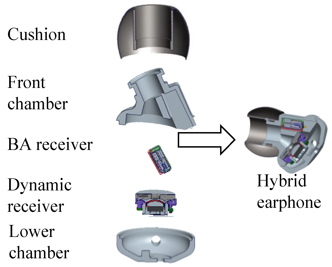
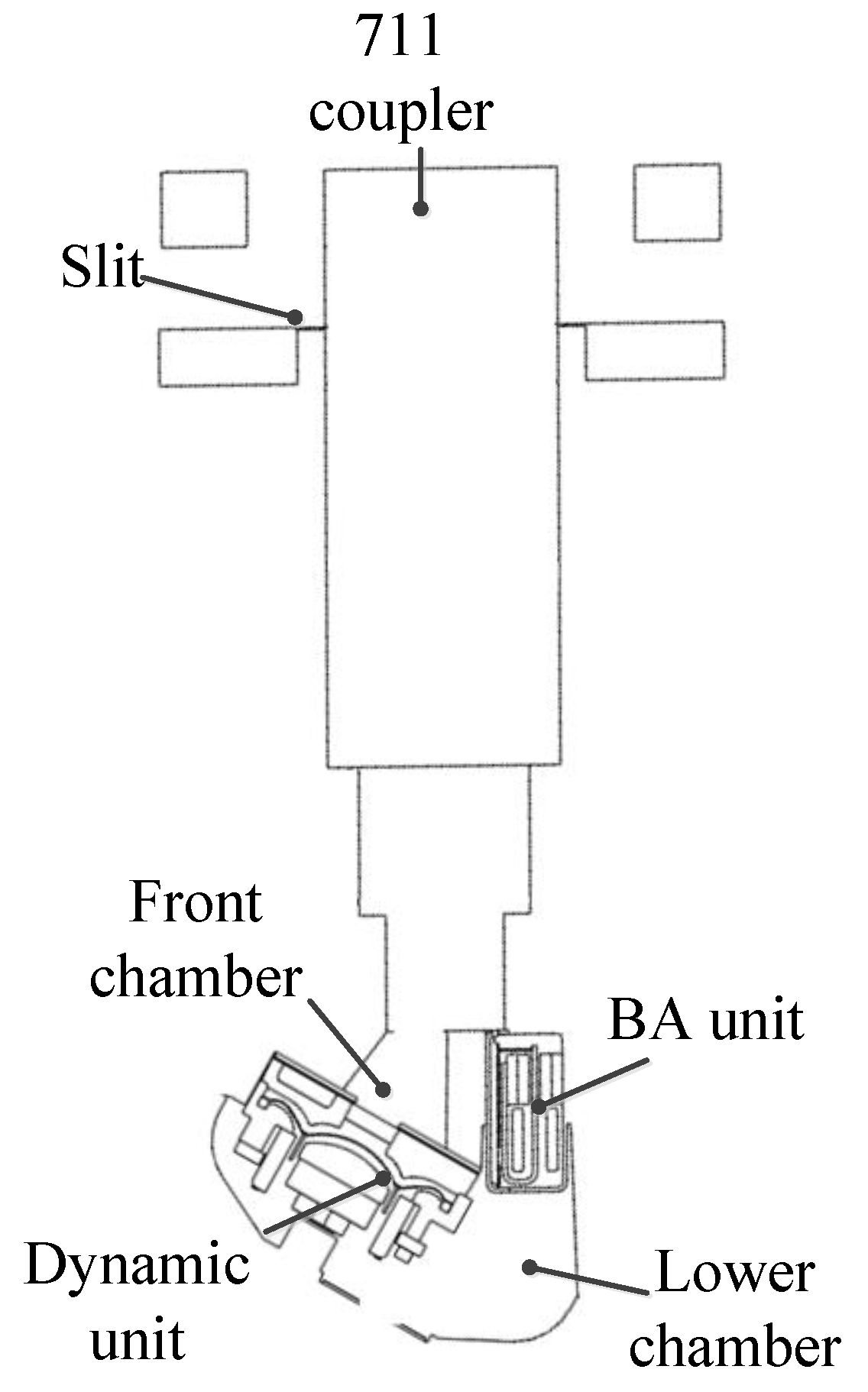
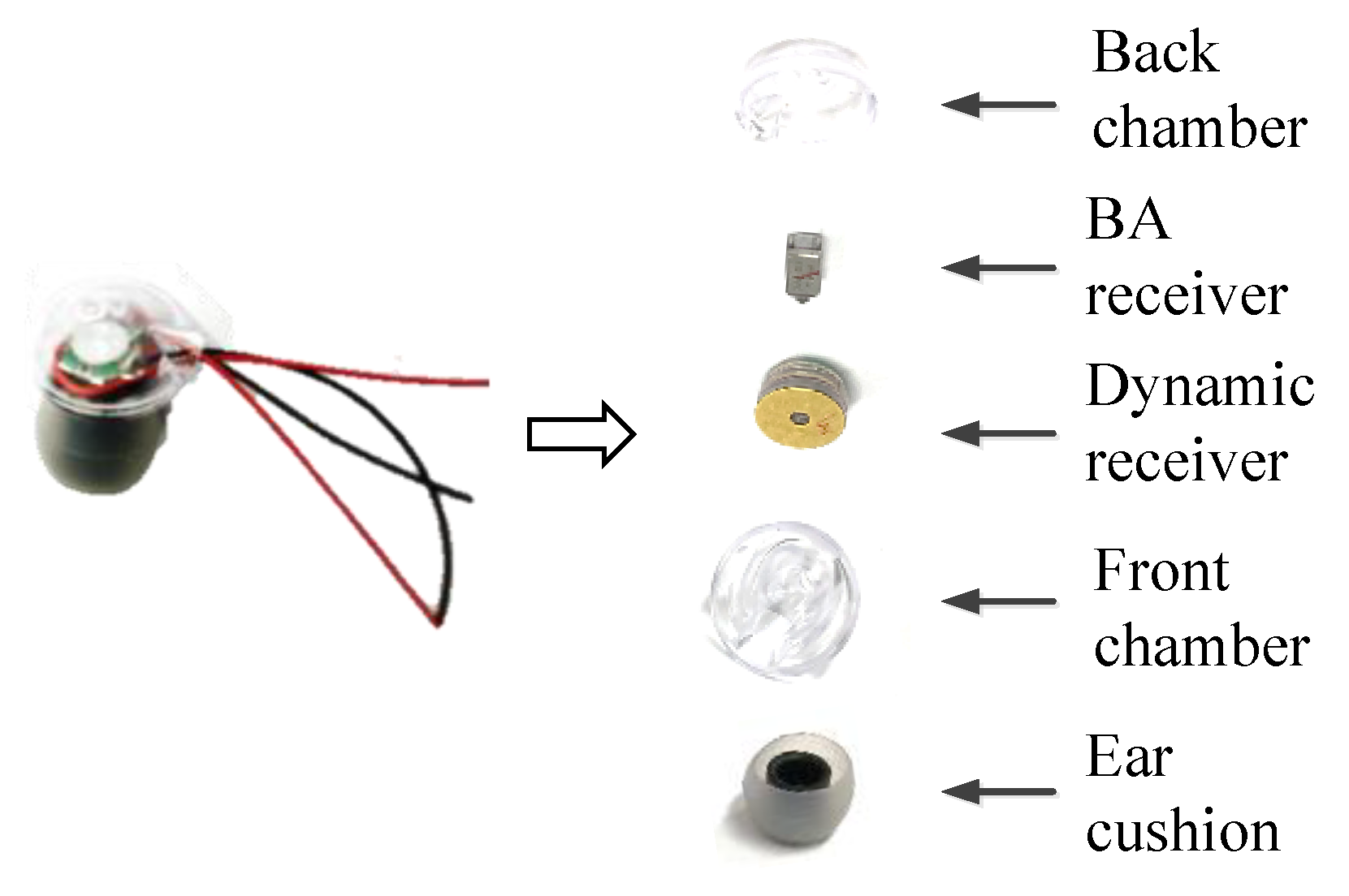
Nowadays, earphones are inseparable companions of multimedia devices such as mobile phones, notebook computers, video recorders, dictation devices, personal digital assistants, MP4 players, and personal music systems. The acoustic transducers generally used in these earphones include microelectromechanical system (MEMS) receivers [1,2], dynamic receivers [3], and balanced-armature (BA) receivers [4,5]. In this work, the BA receiver and dynamic receiver were combined in a hybrid earphone to improve the sound pressure level (SPL) over a wide range. The hybrid earphone components are depicted in Figure 1. The BA receiver and dynamic receiver were inserted in the front chamber, and both shared the same sound-propagation duct. The hybrid earphone can combine the advantages of the BA and dynamic earphones.

Figure 1.
Hybrid earphone components.
Some previous works had developed an analytical method to measure the performance of earphones. Because the electromagnetic, mechanical, and acoustic domain characteristics can be described by the second-order partial differential equation, which can be modeled by an equivalent circuit [6,7], the lumped-parameter method (LPM) was used in the analysis [8,9]. Based on the LPM, the coupling between the headphone and ear was investigated in artificial ears and models. The influence of the back volume was also considered in the analysis [10]. A model of a dynamic driver in an enclosure was developed using the lumped-parameter analysis and analogous circuits [11]. Because the LPM model considers every acoustic structure as a circuit unit, such as capacitance or resistance, the acoustic structure should have an ideal regular shape such as a cylinder or rectangular tube. Thus, the LPM has a limitation in that if the acoustic structure is irregular, the LPM will not work. Olive conducted listening tests of various types of earphones to determine the best response curve. Based on his research, the target curve for an insert earphone was defined [12,13]. To improve the performance of earphones, porous materials were used, and their properties were investigated to check their influence on the SPL of the insert earphone [3].
The previous works have focused on the analysis of dynamic earphones alone. In this work, the hybrid earphone (a combination of dynamic and BA earphones) is analyzed and designed, for the first time, to achieve full-range improved performance. In this analysis, a combination of LPM in the electromagnetic and mechanical domains and finite-element model (FEM) in the acoustic domain is used to model the irregular acoustic structure.
The remainder of this paper is organized as follows: first, the analysis tool for the hybrid earphone is explained in terms of the electromagnetic–mechanical LPM and acoustic FEM. The analysis method is verified by the experiment results. Second, based on the analysis tool, an acoustic tube is optimized to reduce the difference between the analyzed earphones and target SPL. Finally, samples with the optimized tube are manufactured and tested. The root-mean-square value of the SPL deviation of the hybrid earphone is considerably smaller than that of the dynamic and BA earphones.
2. Analysis Method
2.1. Electromagnetic Analysis
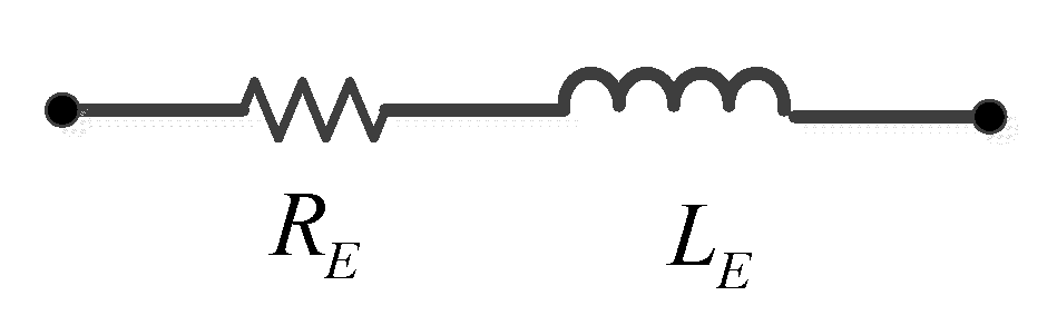
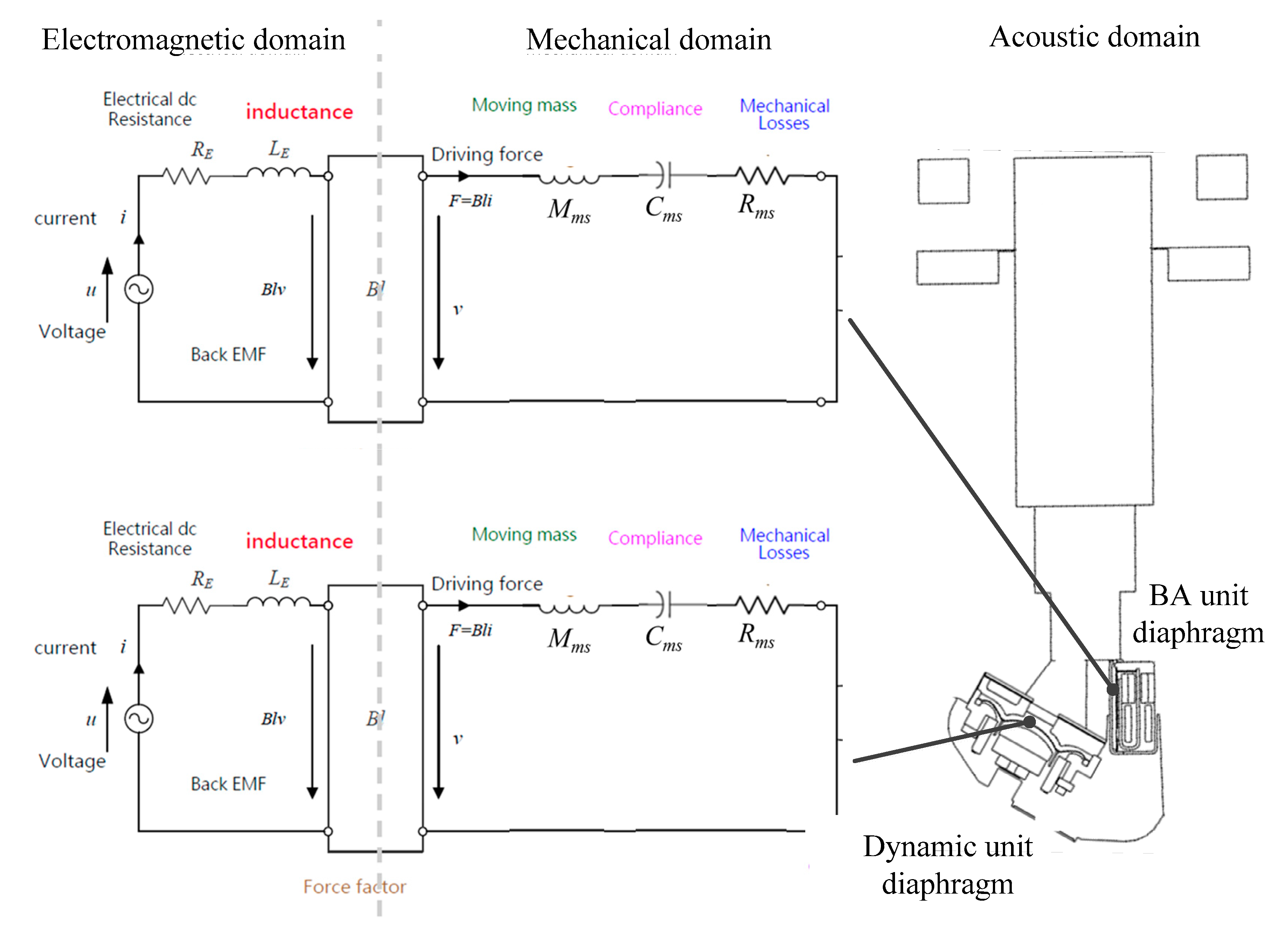
The electromagnetic part is depicted in Figure 2. The mathematical equation is as follows:
where RE is the electrical voice-coil direct current resistance, LE is the voice-coil inductance, and Z is the electrical impedance.

Figure 2.
Equivalent circuit of electromagnetic part.
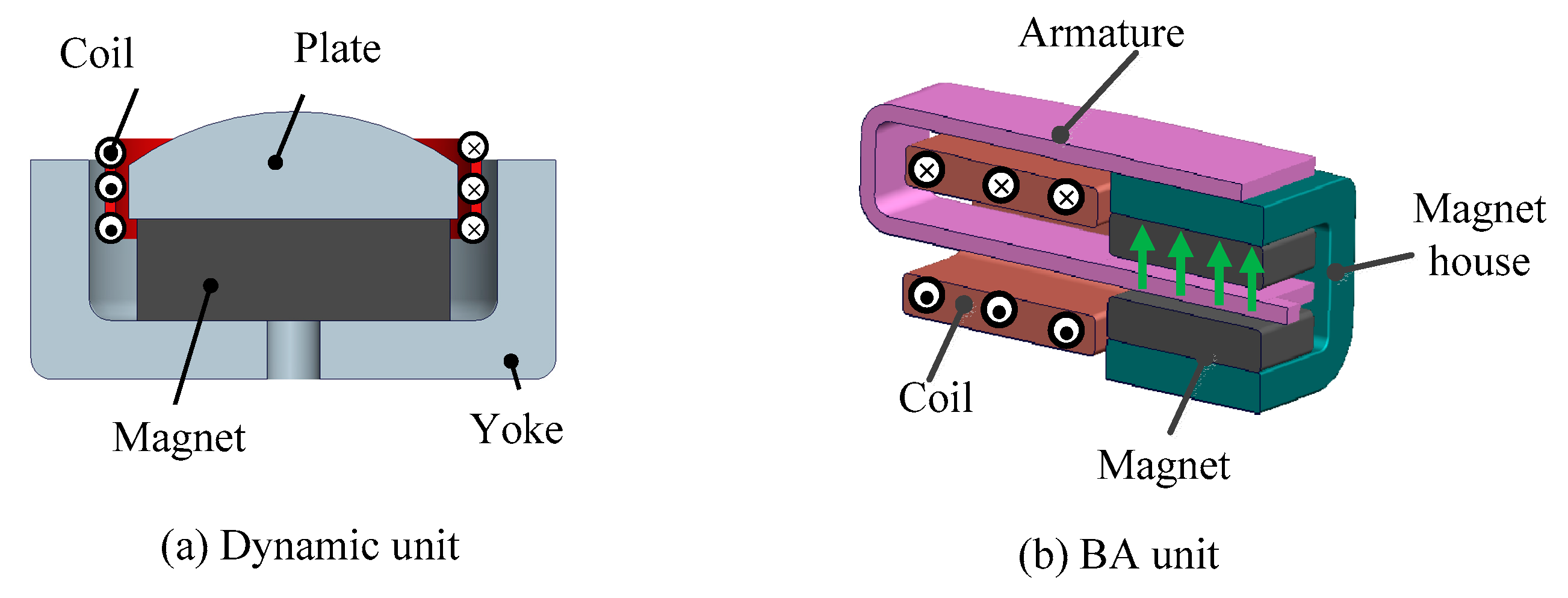
In order to analyze the electromagnetic performance of the dynamic receiver, the three dimension FEM is adopted, as depicted in Figure 3. The flux density in the air gap can be obtained by solving the Maxwell equations. For the dynamic receiver, the force factor is defined as the product of flux density and coil length. For the BA receiver, the force factor is defined as the current force divided by the current [4].
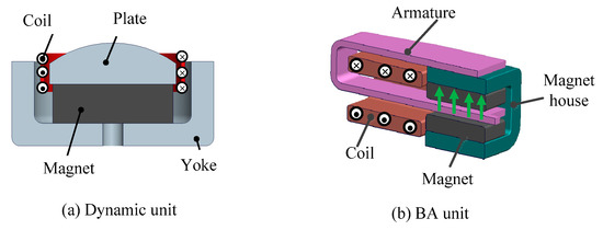
Figure 3.
Electromagnetic domain boundary conditions.
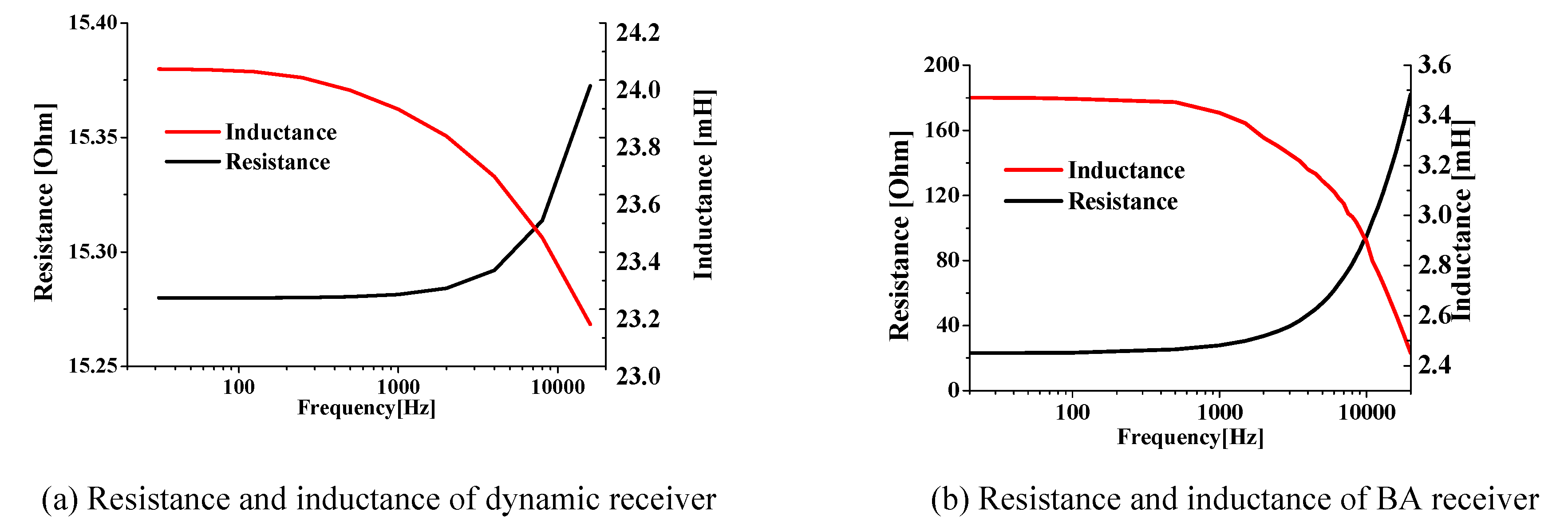
To solve the resistance and inductance, the transient electromagnetic FEM is used. The input is the voltage in the time domain. The permanent magnet’s influence on flux density is considered in the electromagnetic domain. The voltage is the input in the coil. After the transient electromagnetic FEM is solved, the current waveform in the coil is obtained. Based on the voltage waveform and current waveform, the coil impedance is solved. The impedance consists of inductance and resistance, which is shown in Equation (2). Figure 4 demonstrates the inductance and resistance change in terms of frequency. Because of a more serious eddy current, the resistance and inductance of the BA receiver have more change compared with dynamic receivers.
where w, ZE, LE, and RE are the angular frequency, impedance, inductance, and resistance, respectively. The real part is resistance. The imaginary part is the product of inductance and angular frequency.
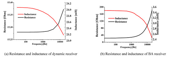
Figure 4.
Calculated resistance and inductance.
2.2. Mechanical Analysis
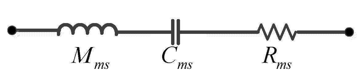
The mechanical domain is modeled as the classical mass–spring system. The 1–degree-of-freedom (DOF) vibration system depicted in Figure 5 is adopted for the mechanical domain.

Figure 5.
Equivalent circuit of mechanical domain.
The governing equation is as follows:
where Mms is the mechanical mass of the vibration system, Rms is the mechanical resistance of the total driver losses, and Cms is the mechanical compliance of the vibration system. To figure out the mechanical parameters, the mechanical FEM is used. The boundary condition is described in Figure 6.
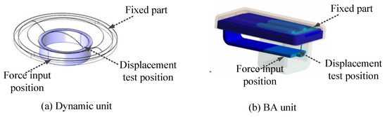
Figure 6.
Mechanical domain boundary conditions.
To figure out the stiffness Kms, the initial force is the input. By solving the mechanical FEM equation, the displacement can be tested. Then, the stiffness is calculated as the force divided by the displacement.
The resonance frequency can be obtained by performing a modal simulation of the mechanical system, and the mass can be calculated using the following equation
Using the parameter-identification method described above, the electromagnetic and mechanical parameters are obtained and are listed in Table 1.

Table 1.
Parameters of the dynamic speaker unit.
2.3. Acoustic Analysis
The acoustic model of a hybrid earphone includes the following parts: the air region in the test jig (IEC 60711 coupler), front chamber, back chamber, dynamic unit, and BA unit. The acoustic model of hybrid earphone is depicted in Figure 7. Based on the dimension differences, different acoustic parts use different acoustic analysis methods to obtain accurate results and save time.

Figure 7.
Acoustic model of the hybrid earphone.
2.3.1. Standard Acoustic Modeling
Acoustic waves are created by the propagation of small linear fluctuations in pressure over a background stationary (atmospheric) pressure [14]. The governing equations is
where w is angular frequency, ρ0 is the background density, u is the node velocity, c is the sound velocity. In the standard acoustic modeling, the acoustic pressure of every node can be solved by inputting the appropriate velocity boundary conditions. To save time, the air region in the 60711 coupler chamber, front chamber, and lower chamber are modeled using the standard acoustic model.
2.3.2. Thermal Acoustic Modeling
For the standard acoustic simulation, assumptions are made to simplify the equations. The system is assumed as lossless and isentropic (adiabatic and reversible). If both the viscous and heat-conduction effects are maintained [15,16,17], the continuity equation of the thermo viscous acoustics in the frequency domain is
where ρ is the density.
The momentum equation is
where µ is the dynamic viscosity, μB is the bulk viscosity, u is velocity, p is sound pressure, and I is the identity tensor.
The energy-conservation equation is
where Cp is the heat capacity at constant pressure, k is the thermal conductivity, α0 is the coefficient of thermal expansion (isobaric), and Q is a possible heat source; and finally, the linearized equation of state, which relates the variations in pressure, temperature, and density, is given by
where βT is the isothermal compressibility. If the acoustic component dimensions are similar to those of the viscous and thermal boundary layers, velocity and temperature gradients will be present at the boundaries of the walls. The viscous loss energy and thermal loss energy per unit volume are described in the following equation:
where τ is the viscous stress tensor. T0 is the background equilibrium temperature. It can be concluded that the energy loss is related to the velocity and temperature gradients. The energy loss contributes to the acoustic energy attenuation. Therefore, the thermal acoustic model needs to be considered when the acoustic component dimension is small. There are four slits in the IEC-60711 coupler. The slit heights cannot be ignored when compared to the thickness of the boundary layer. Therefore, the slits must be modeled in terms of the thermal acoustics.
2.3.3. Narrow-Region Acoustics
The thermal acoustic model involves five DOFs—temperature, sound pressure, and velocity in three directions. Therefore, the thermal acoustic model is time consuming. To obtain a more efficient simulation method, narrow-region acoustics are used. The narrow-region acoustics can be used when the acoustic component is regular. The acoustic tube in front of the dynamic unit will use a circular type in the optimization procedure, which can be modeled by the narrow-region acoustics. The circular duct model is based on a low reduced frequency model that describes the propagation of acoustic waves in small waveguides (ducts and slits), including thermal and viscous losses. In a narrow waveguide, the complex wave number, kc, and complex specific acoustic impedance, Zc, are given by [18,19]
The fluid density ρ, speed of sound c, and angular frequency w define the free-space wave number k0 and specific acoustic impedance Z0. The relationships can be k0 = w/c, Z0 = ρc. γ is the ratio of specific heats. In addition, Ψv, and Ψh are geometry and material-dependent functions, which can be derived by solving the full set of linearized Navier–Stokes equations by splitting these into an isentropic (adiabatic), a viscous, and a thermal part.
2.4. Multiphysics Coupling Modeling
2.4.1. Electromagnetic–Mechanical Coupling
The electromagnetic domain and mechanical domain are coupled by the force factor. On the one hand, the electromagnetic current contributes to the vibration force of the driver unit. The electromagnetic force can be calculated as
where F is the vibration force, Bl is the force factor, and i is the current. In the above equation, the current is solved in the electromagnetic domain. On the other hand, the mechanical vibration velocity can influence the electromagnetic domain. The velocity can contribute to a back electromotive force (emf), which can be calculated as
where V is the back electromotive force, and u is the velocity. In the above equation, the velocity is solved by the 1-DOF equation in the mechanical domain.
F = Bli,
2.4.2. Mechanical–Acoustic Coupling
The mechanical domain and acoustic domain are coupled by the diaphragm. For the acoustic domain, the input is the acceleration, which is in a direction normal to the diaphragm of the dynamic unit and BA unit. The acceleration is solved from the mechanical domain and is described as
The coupling between the mechanical and acoustic domains is the back-chamber acoustic pressure, which is based on the front-chamber acoustic simulation. The velocity of the diaphragm is the source of sound pressure. By solving the standard acoustic governing equation, the sound pressure can be solved with the acceleration input. The pressure is calculated in the following equations
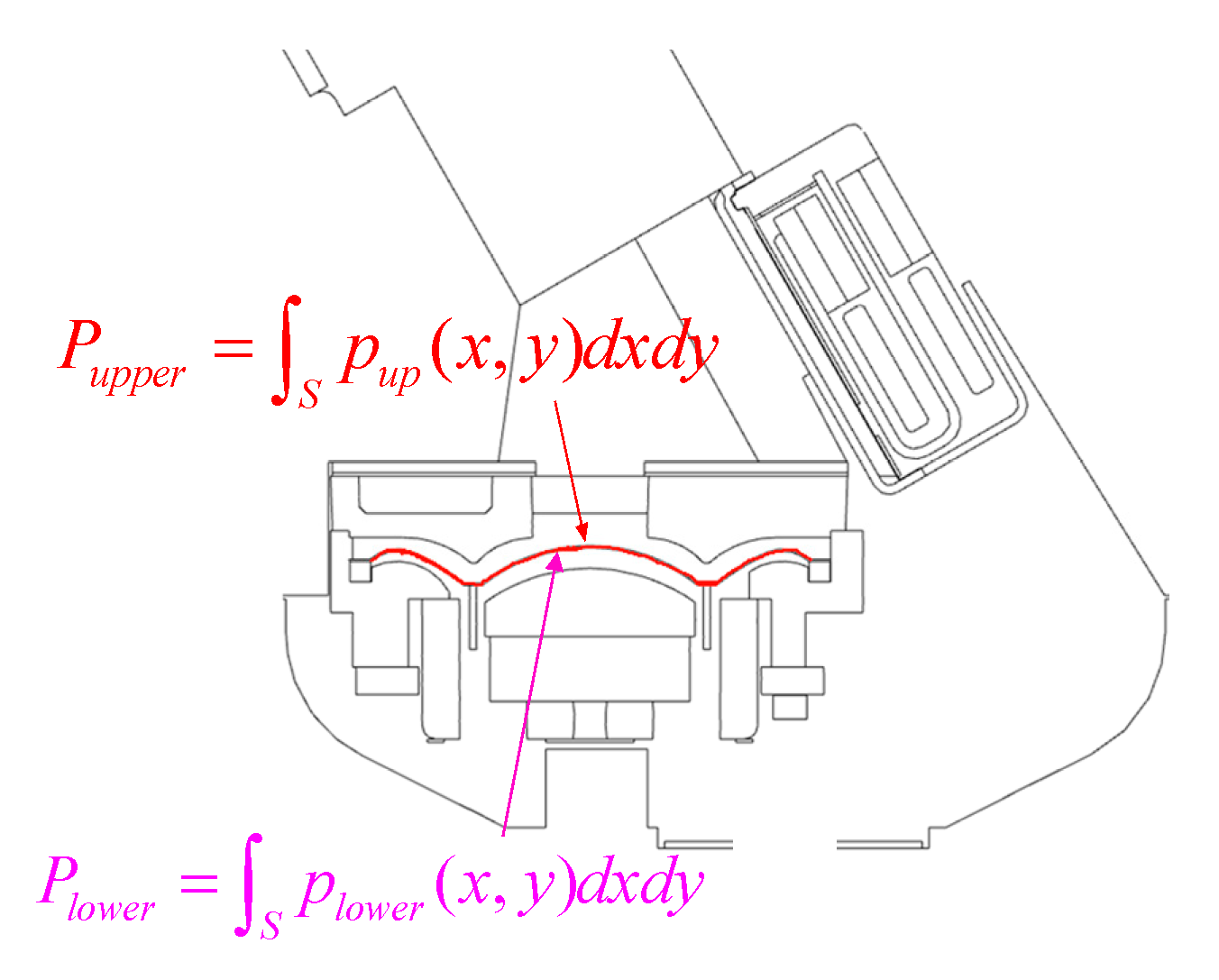
If the diaphragm vibrates up and down, the air pressure forces in the back and front chambers will change. The back chamber and front chamber air pressures are defined as Plower and Pupper, respectively. Plower and Pupper are obtained by integrating the node pressure force over the diaphragm surface. The difference between the pressures is defined as Pair. The air pressure force is depicted in Figure 8. In addition, a current force drives the unit except for the air pressure force. The current force is defined as Fcurrent. The total force acting on the vibration system is F. It can be concluded that the total force can influence the mechanical velocity. Therefore, the mechanical domain and acoustic domain are considered to be coupled with each other.
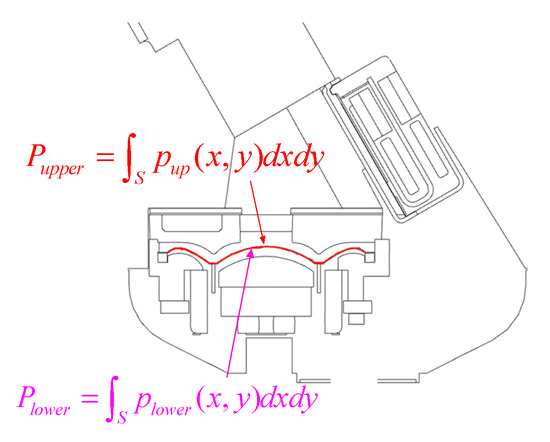
Figure 8.
Air pressure force definition.
The analysis tool is described in Figure 9. In the electromagnetic and mechanical domains, the dynamic and BA units are modeled separately. In the acoustic domain, the dynamic and BA units share the front chamber. In other words, the sound radiated by the BA unit will reach the acoustic cavity in the dynamic unit.
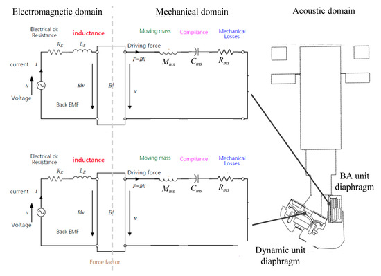
Figure 9.
Analysis tool for hybrid earphone.
3. Experiment
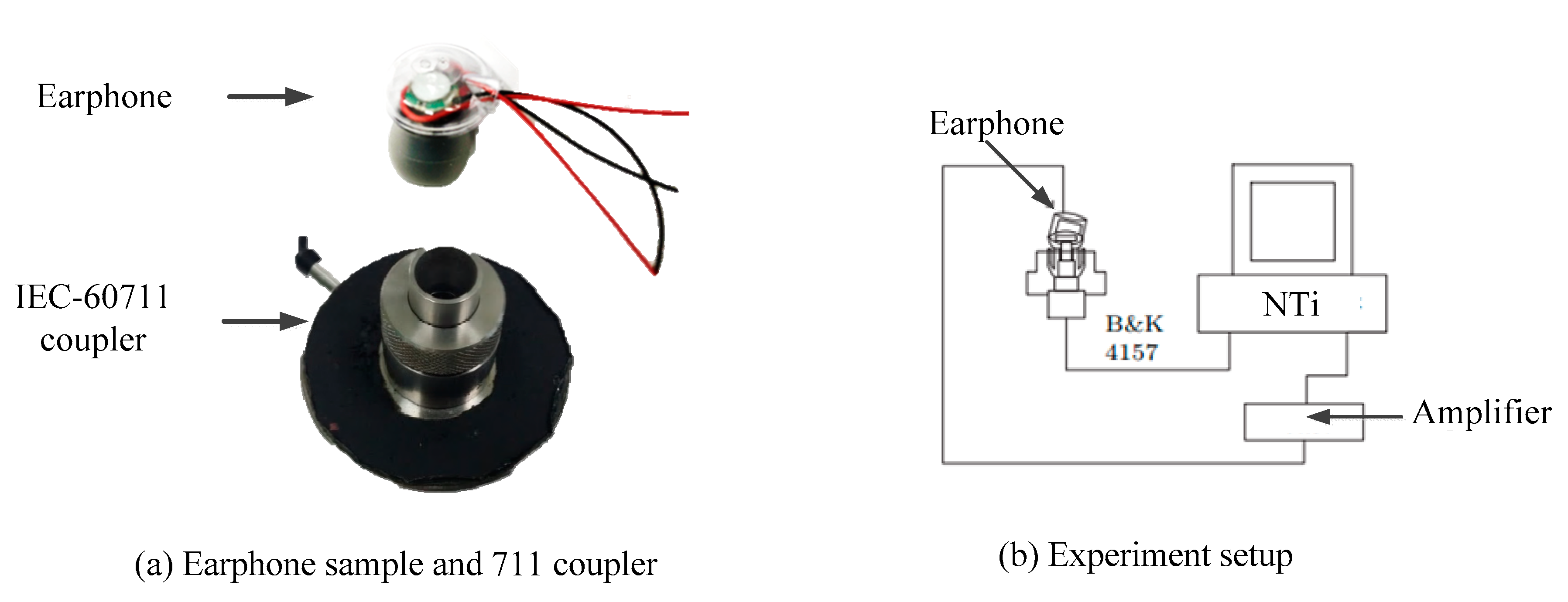
To verify the performance of the hybrid earphone, prototypes were manufactured. Figure 10 presents the sample parts, and Figure 11 shows the sample experiment jig and the setup for the SPL experiment. An NTI system (NTi Audio AG, Schaan, Liechtenstein) was used in the experiments. The IEC-60711 (GRAS, Holte, Denmark) was used to detect the SPL of the earphone. The testing frequency range was from 20 Hz to 20 kHz. A swept sinusoidal signal was used. In the NTI system, the received sound signal was transformed to the frequency domain by the fast Fourier transform.
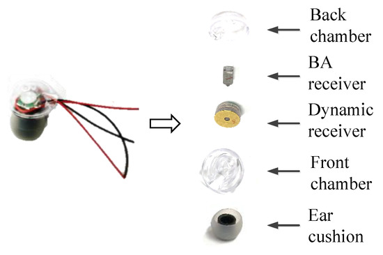
Figure 10.
Components of the earphone.

Figure 11.
Sample and experiment setup.
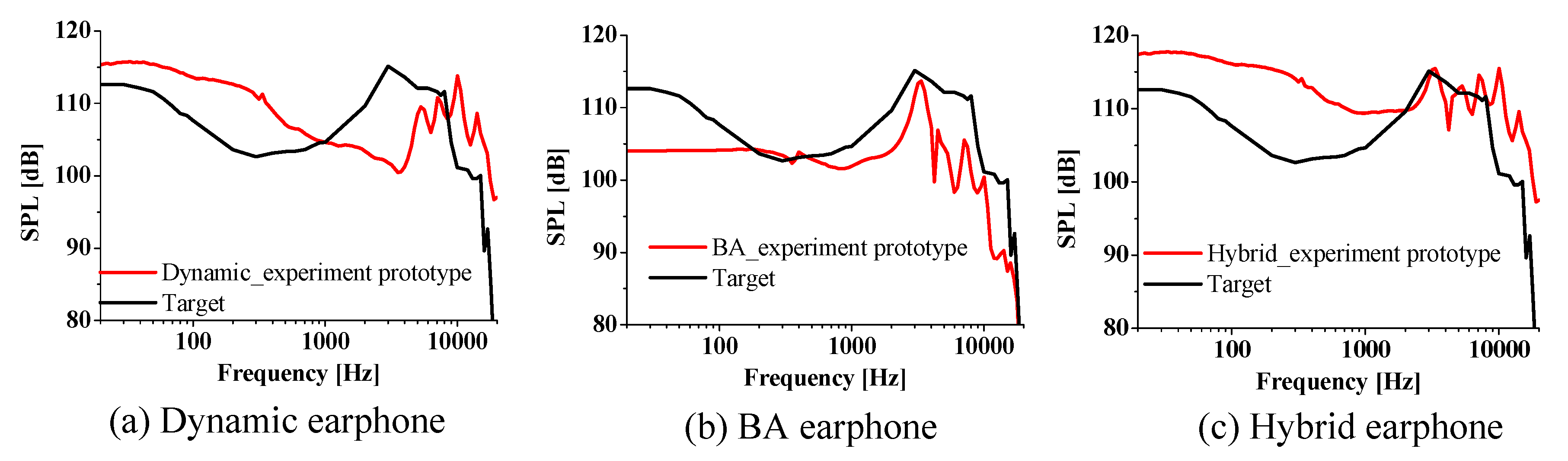
The simulation results can be obtained using the analysis tool and 3D modeling. The dynamic earphone, BA earphone, and hybrid earphone are defined in Table 2. Figure 12 shows the comparison between the experimental and simulated SPL results. The comparison shows that the simulation method can be verified by the experiment. Figure 13 shows the comparison between dynamic, BA, hybrid earphone SPL and the target curve. The target curve is from the previous research by Olive [12,13]. According to Figure 13, the SPL of a hybrid earphone can be treated as the summation of the SPLs of the dynamic and BA earphones. In addition, the dynamic, BA, and hybrid earphones have the same peak frequency in the SPL curve because they have the same front chamber. The SPLs of the dynamic, BA, and hybrid earphones are all different from that of the target earphone.
Table 2.
Earphone definition and root-mean-square value of sound pressure level (SPL) deviation.
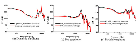
Figure 12.
Earphone sound pressure level (SPL) comparison between experiment and simulation.
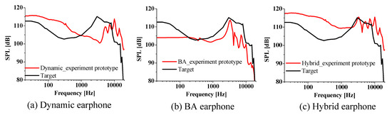
Figure 13.
Earphone experiment results and SPL target.
To quantify the performance of the earphone from 20 to 20 k, the root-mean-square value of SPL deviation is used. The SPL deviation is defined as the SPL difference from the target curve over the region from 20 to 20 k. The equation for SPL deviation is described as follows:
where y and ytarget are the SPL value of the designed earphone and target SPL value, respectively. The root-mean-square value of the SPL deviation for the dynamic, BA, and hybrid earphones with the prototype acoustic tube are 8.94, 6.04, and 9.70, respectively.
According to the comparison between the analyzed earphone SPL curve and target SPL curve, the BA earphone has the best performance at high frequencies. Therefore, the BA earphone will be responsible for the high-frequency components, and the dynamic earphone will be responsible for the low-frequency components. To realize this, the acoustic tube in front of the dynamic receiver needs to be designed again.
4. Acoustic Tube Design
To check the influence of tube on hybrid earphone SPL, the acoustic tube position and acoustic tube diameter were investigated.
4.1. Tube Position Influence
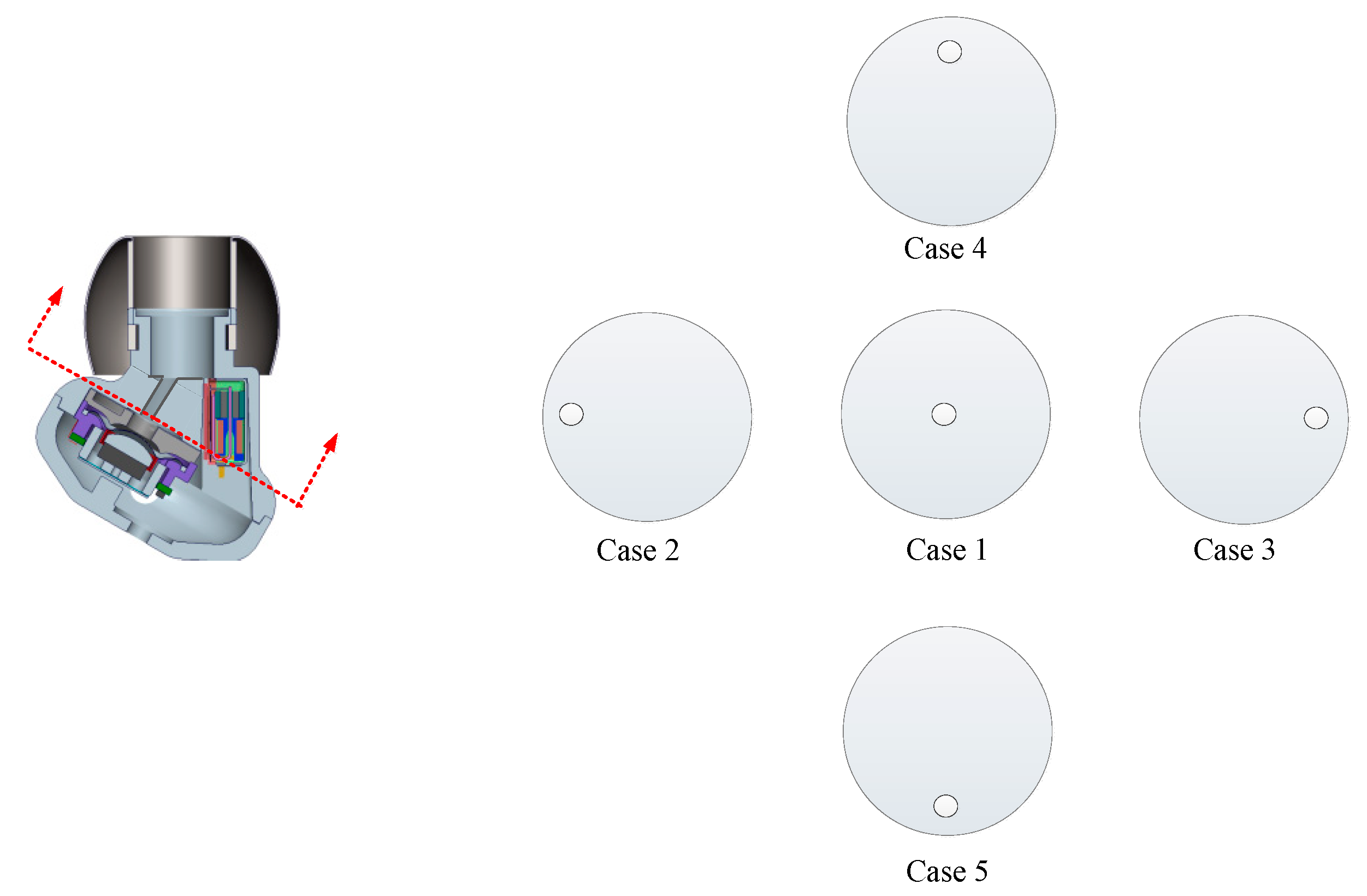
The acoustic tube position influence is depicted in Figure 14. The acoustic tube can be treated as the acoustical mass and acoustical resistance. The acoustical mass has the function of blocking the high-frequency response of the dynamic earphone. Figure 15 demonstrates the results of the tube position influence. It can be concluded that the tube position has no influence on the frequency response of the hybrid earphone.
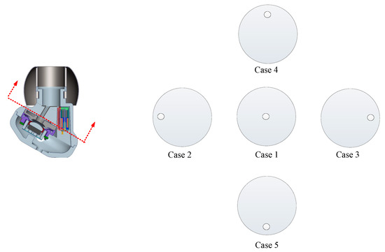
Figure 14.
Acoustic tube position definition.
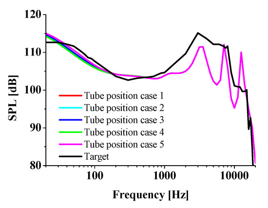
Figure 15.
Acoustic tube position influence and target SPL (simulation result).
4.2. Tube Diameter Influence
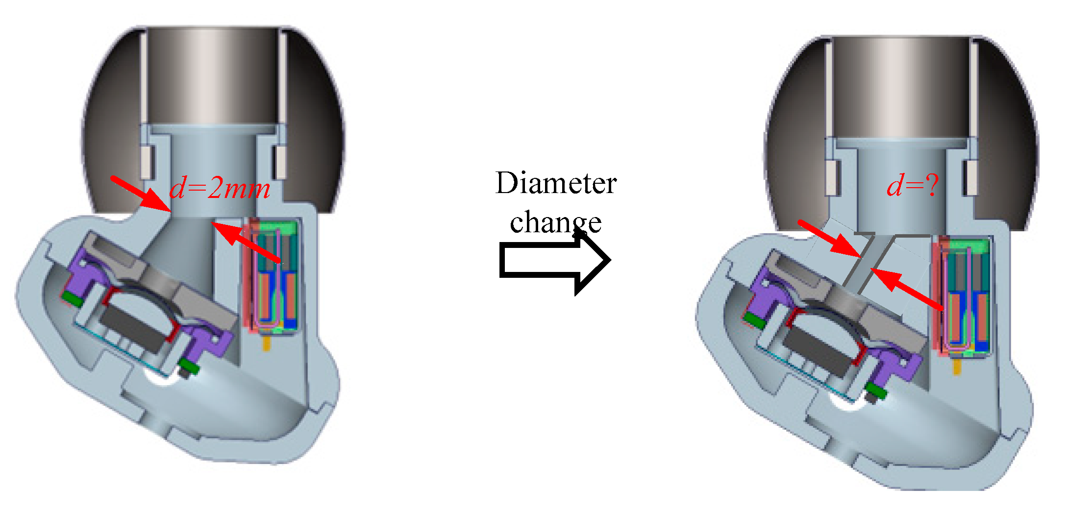
The acoustic tube diameter influence is depicted in Figure 16. Figure 17 demonstrates the results of the tube diameter influence. It can be concluded that when the tube diameter increases, the low frequency response of hybrid earphone increases.

Figure 16.
Acoustic tube diameter definition.
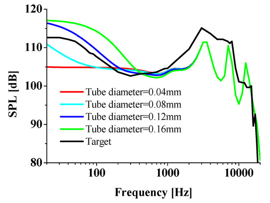
Figure 17.
Acoustic tube diameter influence and target SPL (simulation result).
4.3. Tube Optimization
According to the sensitivity analysis of the tube position and tube diameter, the tube position almost has no influence on hybrid earphone SPL. So, a tube diameter change is treated as the method to improve the SPL of the hybrid earphone.
The diameter determination is accomplished by optimization. According to the manufacture precision and tube-space limitations, the diameter is selected between 0.1 mm and 2 mm. The objective function is the difference between the analyzed SPL and the Harman target curve, which is defined by the following equation
To minimize the difference between the analyzed hybrid earphone SPL and target SPL, the Nelder–Mead algorithm is used to determine the tube diameter [20]. The optimized diameter is determined to be 0.1 mm. The sound tube is manufactured according to the determined diameter and is inserted in front of the dynamic unit. The SPL of the hybrid earphone with an optimized acoustic tube is presented in Figure 18. It can be concluded that the acoustic tube blocks the high-frequency sound pressure of the dynamic unit. The low-frequency sound energy goes through the tube and is combined with the sound of the BA unit. The high-frequency response of the hybrid earphone is from the BA unit. By combining the dynamic and BA units, the hybrid earphone can match the target SPL.

Figure 18.
SPL of earphone with optimized acoustic tube and target SPL (simulation result).
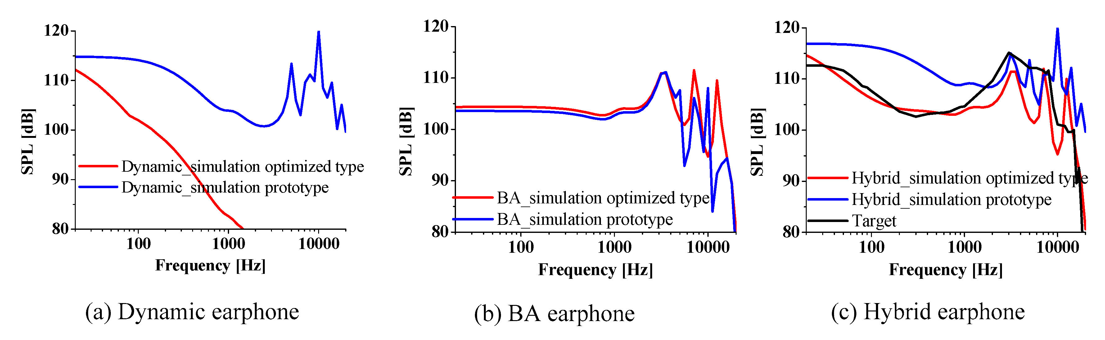
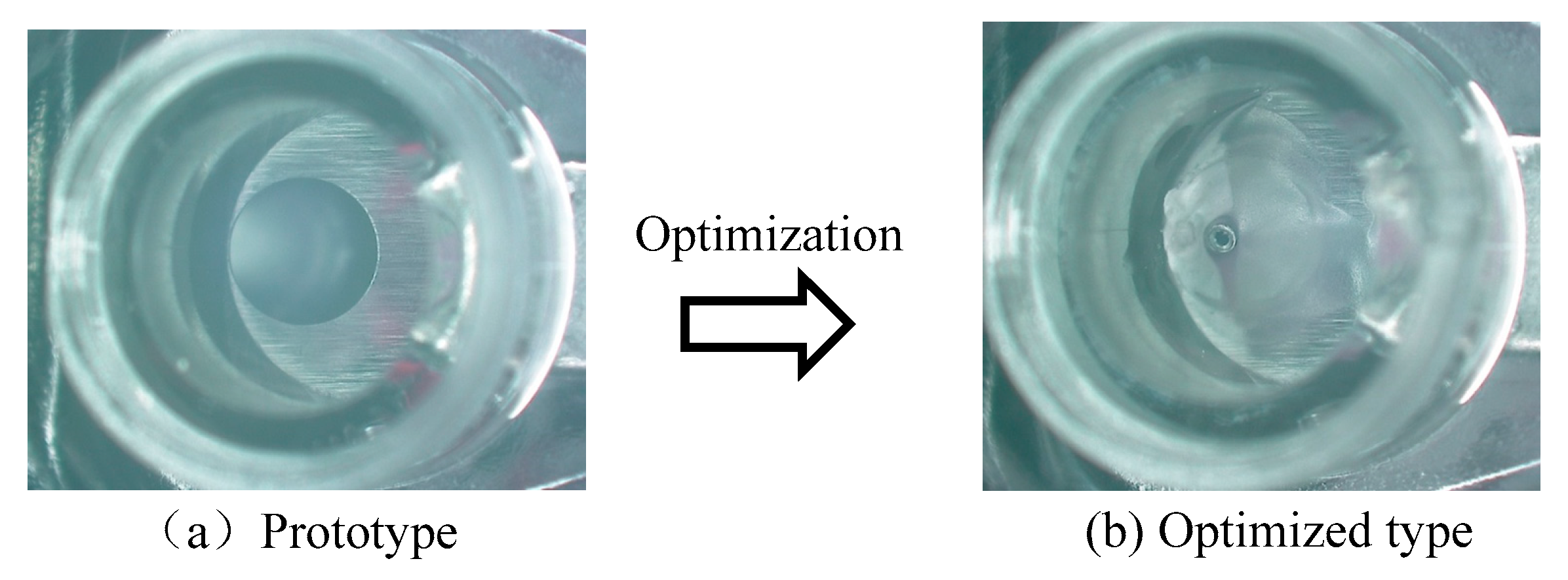
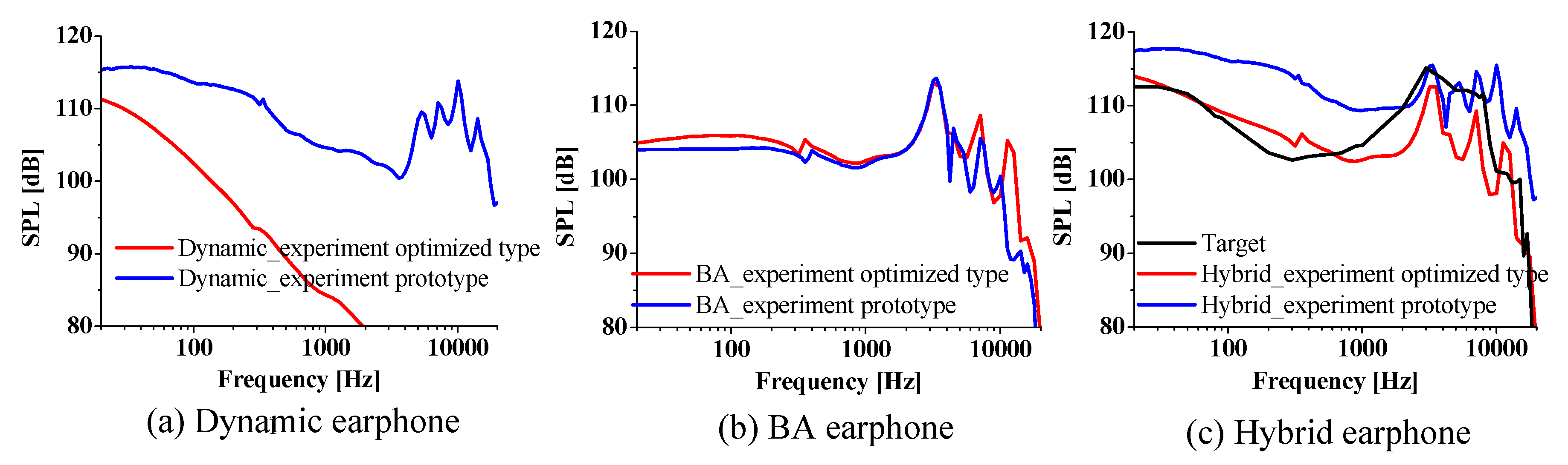
The acoustic tube is manufactured based on the simulated diameter. The samples are shown in Figure 19. After the optimized tube is used in the front chamber, the dynamic and BA units work together to produce sound. Figure 20 depicts the SPL experiment results of the dynamic, BA, and hybrid earphones with the acoustic tube (optimized type and prototype). After the optimized acoustic tube is used, the high-frequency response of the dynamic earphone does not exist. The BA earphone is responsible for the high-frequency response. The dynamic earphone improves the low-frequency response.
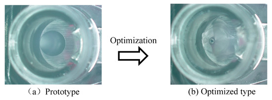
Figure 19.
Acoustic tube in front chamber (prototype and optimized type).
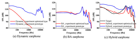
Figure 20.
SPL of earphone with acoustic tube (optimized type and prototype) and target SPL (experiment result).
The root-mean-square value of the SPL deviation for the earphone with the optimized acoustic tube is calculated to be 4.60. Thus, it is found that the full-range response is improved when the hybrid earphone with the optimized acoustic tube is used.
5. Conclusions
This work modeled the dynamic earphone and BA earphone in the electromagnetic and mechanical domains using LPM and in the acoustic domain using FEM, to analyze the SPL. The analysis tool was verified through experiments performed on the dynamic earphone, BA earphone, and hybrid earphone. According to the experimental SPL results, the difference in the RMS values of SPLs of the dynamic, BA, and hybrid earphones, with a prototype acoustic tube, were 8.94, 6.04, and 9.70, respectively. To decrease the difference in the RMS SPL values and improve the full-range performance of the hybrid earphone, an acoustic tube was optimized based on the analysis tool and the Nelder–Mead optimization algorithm. The diameter of the optimized acoustic tube was determined to be 0.1 mm. After applying the acoustic filter, the difference in the RMS value of the hybrid earphone became 4.60.
Author Contributions
Data curation, Y.-W.J. and J.-H.K.; Formal analysis, Y.-W.J., D.-P.X. and Z.-X.J.; Funding acquisition, S.-M.H.; Investigation, Y.-W.J. and D.-P.X.; Methodology, Y.-W.J. and D.-P.X.; Project administration, Y.-W.J. and S.-M.H.; Resources, Y.-W.J. and D.-P.X.; Software, Z.-X.J. and J.-H.K.
Funding
This research received no external funding.
Conflicts of Interest
The authors declare no conflict of interest.
References
- Zhao, C.; Knisely, K.E.; Grosh, K. Design and fabrication of a piezoelectric MEMS xylophone transducer with a flexible electrical connection. Sens. Actuators A Phys. 2018, 275, 29–36. [Google Scholar] [CrossRef]
- Zhao, C.; Knisely, K.E.; Grosh, K. Modeling, Fabrication, and Testing of a MEMS multichannel aln Transducer for a Completely Implantable Cochelar Implant. In Proceedings of the 2017 19th International Conference on Solid-State Sensors, Actuators and Microsystems, Kaohsiung, Taiwan, 18–22 June 2017; pp. 16–19. [Google Scholar]
- Tsai, Y.T.; Shiah, Y.C.; Huang, J.H. Effects of porous materials in an insert earphone on its frequency response-experiments and simulations. IEEE Trans. Ultrason. Ferroelectr. Freq. Control 2012, 59, 2537–2547. [Google Scholar] [PubMed]
- Xu, D.P.; Lu, H.W.; Jiang, Y.W.; Kim, H.K.; Kwon, J.H.; Hwang, S.M. Analysis of sound pressure level of a balanced armature receiver considering coupling effects. IEEE Access 2017, 5, 8930–8939. [Google Scholar] [CrossRef]
- Jiang, Y.W.; Xu, D.P.; Hwang, S.M. Electromagnetic-mechanical analysis of a balanced armature receiver by considering the nonlinear parameters as a function of displacement and current. IEEE Trans. Magn. 2018, 54, 1–4. [Google Scholar]
- Bauer, B.B. Equivalent circuit analysis of mechano-acoustic structures. J. Audio Eng. Soc. 1976, 24, 643–652. [Google Scholar]
- Leach, W.M., Jr. Analogous circuits for acoustical systems and analogous circuits for mechanical systems. In Introduction to Electroacoustic and Audio Amplifer Design, 3rd ed.; Kendall Hunt Publishing: Dubuque, IA, USA, 2003; pp. 33–62. [Google Scholar]
- Huang, C.H.; Pawar, S.J.; Hong, Z.J.; Huang, J.H. Insert earphone modeling and measurement by IEC-60711 coupler. IEEE Trans. Ultrason. Ferroelectr. Freq. Control 2011, 58, 461–469. [Google Scholar] [CrossRef] [PubMed]
- Huang, C.H.; Pawar, S.J.; Hong, Z.J.; Huang, J.H. Earbud-type earphone modeling and measurement by head and torso simulator. Appl. Acoust. 2012, 73, 461–469. [Google Scholar] [CrossRef]
- Blanchard, L.; Agerkvist, F. Concha Headphones and Their Coupling to the Ear. In Audio Engineering Society Convention 126; Audio Engineering Society: New York, NY, USA, 2009. [Google Scholar]
- Avis, M.R.; Kelly, L.J. Principles of Headphone Design—A Tutorial Review. In Audio Engineering Society Conference: UK 21st Conference: Audio at Home; Audio Engineering Society: New York, NY, USA, 2006. [Google Scholar]
- Olive, S.; Welti, T.; Khonsaripour, O. The Preferred Low Frequency Response of In-Ear Headphones. In Proceedings of the Audio Engineering Society Conference: 2016 AES International Conference on Headphone Technology, Aalborg, Denmark, 24–26 August 2016. [Google Scholar]
- Olive, S.; Welti, T.; Khonsaripour, O. The Influence of Program Material on Sound Quality Ratings of In-Ear Headphones. In Proceedings of the 142nd Audio Engineering Society Convention, Berlin, Germany, 20–23 May 2017. [Google Scholar]
- Kinsler, L.E.; Frey, A.R.; Coppens, A.B.; Sanders, J.V. Fundamentals of Acoustics, 4th ed.; Wiley-VCH: Weinheim, Germany, 1999. [Google Scholar]
- Nijhof, M.J.J. Viscothermal Wave Propagation. Ph.D. Thesis, University of Twente, Drienerlolaan, The Netherlands, 2010. [Google Scholar]
- Kampinga, W.R. Viscothermal Acoustics Using Finite Elements-Analysis Tools for Engineers. Ph.D. Thesis, University of Twente, Drienerlolaan, The Netherlands, 2010. [Google Scholar]
- Beltman, W.M.; Van der Hoogt, P.J.M.; Spiering, R.M.E.J.; Tijdeman, H. Implementation and experimental validation of a new viscothermal acoustic finite element for acousto-elastic problems. J. Sound Vib. 1998, 216, 159–185. [Google Scholar] [CrossRef]
- Myers, M.K. Transport of energy by disturbances in arbitrary steady flows. J. Fluid Mech. 1991, 226, 383–400. [Google Scholar] [CrossRef]
- Stinson, M.R. The propagation of plane sound waves in narrow and wide circular tubes, and generalization to uniform tubes of arbitrary cross-sectional shape. J. Acoust. Soc. Am. 1991, 89, 550–558. [Google Scholar] [CrossRef]
- Conn, A.R.; Scheinberg, K.; Vicente, L.N. Introduction to Derivative-Free Optimization. Siam. 2009. Available online: https://books.google.com.ph/books?hl=en&lr=&id=7c7X6tlcaHEC&oi=fnd&pg=PP2&dq=Introduction+to+Derivative-Free+Optimization&ots=lmQGro6TxJ&sig=VbiLNrwzTovGcfR5aYbwpLDX184&redir_esc=y#v=onepage&q=Introduction%20to%20Derivative-Free%20Optimization&f=false (accessed on 7 August 2019).


© 2019 by the authors. Licensee MDPI, Basel, Switzerland. This article is an open access article distributed under the terms and conditions of the Creative Commons Attribution (CC BY) license (http://creativecommons.org/licenses/by/4.0/).