Abstract
Aiming at aerodynamic drag reduction for transportation systems, a new active surface is proposed that combines a bionic nonsmooth surface with a jet. Simulations were performed in the computational fluid dynamics software STAR-CCM+ to investigate the flow characteristics and drag reduction efficiency. The SST K-Omega model was used to enclose the equations. The simulation results showed that when the active surface simultaneously reduced the skin friction and overcame the sharp increase of pressure drag caused by a common nonsmooth surface, the total net drag decreased. The maximum drag reduction ratio reached 19.35% when the jet velocity was 11 m/s. Analyses of the turbulent kinetic energy, pressure distribution, and velocity profile variations showed that the active surface reduced the peak pressure on the windward side of the nonsmooth unit cell, thereby reducing the total pressure drag. Moreover, the recirculation formed in the unit cell transformed the fluid–wall sliding friction into fluid–fluid rolling friction like a rolling bearing, thereby reducing the skin friction. This study provides a new efficient way for turbulent drag reduction to work.
1. Introduction
Flow control and drag reduction are important research focuses that should be fully considered in a range of engineering fields. High efficiency of drag reduction can improve propulsion efficiency and reduce fuel consumption [1]. Turbulence is a common flow state in most situations, and the skin friction on the turbulent wall is much greater than that on the laminar wall [2,3]. Therefore, the study of drag reduction in wall turbulence has important practical significance.
To control the flow, a variety of methods have been proposed. Changing the wall conditions by the super-hydrophobic wall was considered as an effective method [4,5]. Changing the fluid properties by adding polymers also achieved control effects [6]. Moreover, the application of external motions and forces to the original wall to generate controllable disturbance and achieve the flow control was also studied [7,8,9]. These methods have achieved certain effects in specific working conditions.
Taking inspiration from nature, researchers started to study the turbulent drag reduction on grooved surfaces, which was inspired by the nonsmooth structures on shark skin. Most studies focused on drag reduction characteristics and its mechanisms [10]. The shape and size of the groove structure were shown to have significant impacts on drag reduction characteristics. Simulations and physical experiments showed that the groove surface can achieve a maximum drag reduction ratio of 10% when the dimensionless spacing (S+) was between 16 and 20 and the dimensionless height (H/S) was between 0.5 and 0.8 [11,12]. A study of an airfoil model with longitudinal microgrooves also showed that the drag reduction effect can be obtained by setting the scale of the micro-groove equal to the scale of the turbulent vortex near the wall [13].
The decrease in the exchange of flow momentum is one of the main causes of drag reduction. Bechert et al. [11] found that the existence of the groove can inhibit the frequency of momentum exchange along the spreading direction. Although the existence of the groove will increase the surface area, the spikes can destroy the streamwise vortex and restrain the spreading motion, thereby restraining the formation of low-speed strips and reducing the turbulent kinetic energy exchange. Moreover, the fluid in the groove valley can be maintained at a low-speed state, and the shear stress in the trough can be greatly reduced, resulting in a net reduction in skin friction [14,15]. Therefore, the drag reduction enhancement mechanism of microgrooves can be considered as the restriction effect [16]. Direct numerical simulations intended to study the relationship between vortices at the bottom of the trench and energy dissipation also confirmed the above conclusions [17]. The existence of the groove will also affect the transition process, which can be a two-dimensional linear process or a three-dimensional process [18].
In recent years, another natural phenomenon, named a “super-hydrophobic surface”, has attracted increasing research interest. This type of surface has significant effects on drag reduction [19,20,21]; so much so that the drag reduction ratio even approached 50% in some experiments with low speed [22]. There are two ways to obtain a super-hydrophobic surface: (1) by modifying a high-surface-energy rough surface with low-surface-energy materials and (2) by constructing a micro-rough structure on a low-surface-energy surface. One of the important ways to study drag reduction characteristics is via direct numerical simulation (DNS). In such simulations, a hydrophobic surface is always represented by a slip boundary condition. When the slip boundary condition was used in the streamwise direction, the skin friction drag decreased. However, when the slip boundary condition was used in the spanwise direction, the drag increased [23,24].
The flow slip on the wall is considered to be the main cause of drag reduction. An average slip velocity of over 75% of the bulk velocity was obtained on a super-hydrophobic surface via DNS, and the corresponding wall shear stress reduction was found to be nearly 40% [25]. The apparent flow slip was verified with a confocal surface metrology system [26,27]. Costantini et al. [28] suggested that the mean slip velocity at the wall increases the flow rate at a fixed pressure drop in turbulent pipe flow. Therefore, slip length is the key to drag reduction that is related to the flow state. In a laminar flow state, the effective slip length only depends on the surface geometry (i.e., the slip length is independent of the Reynolds number). In a turbulent flow state, the effective slip length is a function of the Reynolds number, indicating that the slip length is dependent on the flow conditions near the surface [29].
Some special flow patterns in nature also inspired new drag reduction methods. Sand dune flow is one of the most common flow patterns. Under the transport of wind, grains of sand migrate to inclined windward slopes and deposit on steep slip slopes, thereby forming dunes. Herrmann and Sauermann [30] pointed out that sand dunes are aerodynamic objects because their shape is adapted to allow the air flow with the least effort. Hesp and Hastings [31] also reported that the shape of dunes is directly controlled by aerodynamic processes. The drop-in velocity and shear stress at the base of a dune has been widely predicted and observed [32]. Some researchers have even applied the aerodynamic characteristics of sand dunes to practical engineering applications. Gao and Ning [33] proposed a new barchan dune (BD) vortex generator, which exhibited 75–80% less drag when compared with a V-gutter at the same blockage ratio. Li et al. [34] proposed a new dune-shaped combustion chamber to reduce the total pressure loss and obtain a stable trapped vortex, whose simulation results showed that there is an optimal leeward angle with small total pressure loss.
Shark gills were also adapted as a bionic prototype to reduce drag. As a fast-moving marine animal, sharks can travel very fast during predation. Moreover, sharks have interesting broad gill plates located on the front of the body. Sharks inhale sea water through a half-open mouth, which flows out of the gills to exchange gas; however, the function of these gills is closely related not only to respiration, but also to drag reduction [35]. Lighthill [36] found that fish will close the gill slits on the inside bend during turns and shunt the gill efflux into the gills on the outside bend, a separation-prone region of the body, to obviate separation drag. Babenko and Koval [37] proposed that the orientation and placement of the gill openings are particularly well suited to the jet-blowing technique. Inspired by shark gills, Li et al. [38] studied the drag reduction characteristics of bionic jet surfaces, in which they obtained a maximum drag reduction rate of 9.51%. Similarly, Zhang et al. [39] studied the drag reduction characteristics of a revolving body with a bionic jet surface, in which they achieved a maximum friction reduction rate of 10.8%.
A preceding study on grooved surfaces mostly focused on single V-shaped grooves parallel to the mainstream, only considering some simple morphology for nonsmooth surfaces. Moreover, the maximum drag reduction ratio reached approximately 10%, and it was hard to make further breakthroughs. The microstructures of super-hydrophobic surfaces are micron-sized, which are commonly generated via laser processing. However, from an economic point of view, super-hydrophobic surfaces are not suitable for large-scale applications in engineering fields.
Based on bionics, the current study tried to provide a new drag reduction method. The study broke the limitations in a single morphology and proposed a new nonsmooth surface inspired by sand dunes. The nonsmooth surface can effectively reduce the skin friction. However, the decrease in skin friction was accompanied by a sharp increase in pressure drag. An active surface that combines a bionic nonsmooth surface with a jet was then proposed. The active surface overcame the common problem of the rapid increase in pressure drag in designing nonsmooth surfaces and achieved better drag reduction effects. The study provides a new idea for drag reduction in the next generation of transportation systems.
In the second part of this paper, the physical model of the bionic nonsmooth surface is established and the hypothesis in the calculation process is verified. In the third part, the results of numerical simulations are analyzed, and the drag reduction mechanism of the active surface is explained with three aspects: Turbulent kinetic energy, pressure distribution, and velocity characteristics. A summary of the whole work is made in the last part.
2. Physical Model Establishment and Hypothesis Verification
2.1. Model of A Bionic Nonsmooth Surface
Due to the excellent aerodynamic characteristic, a sand dune was selected as the bionic object of the nonsmooth unit cell (Figure 1).
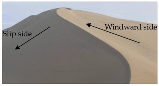
Figure 1.
Morphology of the sand dune.
Claudin et al. [40] studied the sand dune located on the western edge of the Erg Oriental near Merzouga in Eastern Morocco (), where the dune was an elongated dome with no avalanche slip face, showing that no flow separation occurred. According to the measured results, the cross-section of the dune can be expressed by the following Equation:
where is the starting point of the dune, A is the half-height of the dune, and k is the number of waves (the wavelength ). According to Equation (1), the shape equation of the sand dune involves two parameters: The half-height (A) and the wavelength () (Figure 2).
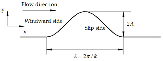
Figure 2.
Mathematical model of the dune.
Preliminary research has found that turbulent drag is most influenced by the near-wall turbulent region of the boundary layer, defined as , where y is the normal distance between the fluid and the wall and is the thickness of the boundary layer [41]. By disturbing the near-wall turbulent region with a nonsmooth unit cell, a new turbulent boundary layer will be generated. It is suggested that the depth of the nonsmooth unit cell (2A) should be smaller than the thickness of the near-wall turbulent region to obtain the best disturbance effect, which can be expressed as follows:
As a result, to satisfy Equation (2), the depth of the nonsmooth unit cell (2A) was defined as 0.0015 m. The wave number was set to 2000; thus, the wavelength (λ) was 0.0031 m. To ensure the stability of the fluid, a flat surface was set behind the nonsmooth unit cell, and the length (d) was set to 0.005 m. The cross-section of the bionic nonsmooth surface is shown in Figure 3.
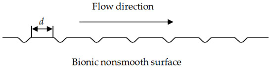
Figure 3.
Cross-section of the bionic nonsmooth surface.
2.2. Computational Domain Selection and Grid Division
The computational domain of the simulations is the same as the classical boundary layer transition experiment [42]. The computational domain has been divided into three sections: An inlet smooth section (surface A), a test section (nonsmooth surface), and an outlet smooth section (surface B), as shown in Figure 4. The total length was set to 1.5 m, and the length of the test section was set to 0.3 m. To form a fully developed turbulent boundary layer at the inlet of the test section, a smooth section with a length of 1 m was arranged upstream. The normal distance from the far field boundary to the wall was 0.2 m.
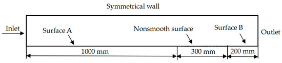
Figure 4.
Computational domain of the numerical simulation.
To ensure that the fully developed turbulent boundary layer was obtained before the test section, the transition model was used to solve the computational domain. Figure 5 shows that the simulation accurately captures the flow transition phenomenon. The location of the transition starting point (point A) and the length of the transition region (region B) are in good agreement with the experimental results. The simulation also shows that the boundary layer in the test section fully developed and became a turbulent boundary layer.
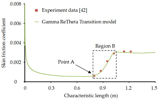
Figure 5.
Of the flow state in the test region.
For the accuracy of the real near-wall flow field, the prism layer grids, which were determined by the thickness of the near-wall cell layer and stretch factor, were adapted (Figure 6), and the grids near the wall were refined. To reach y+ < 1, the thickness of the near-wall cell layer was set to m, and the stretch factor was set to 1.2. In addition, the inlet and outlet areas were also refined (Figure 7).
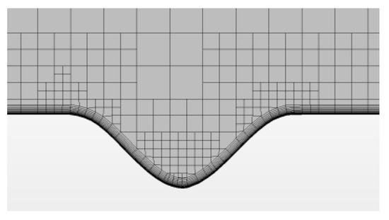
Figure 6.
Inflation layer.
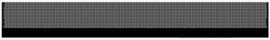
Figure 7.
Grid settings of models.
To verify the independence of the computational grid, the skin friction coefficients of the test section were calculated under five grids with multiple densities (Table 1). The results showed that when the number of grids reached 251,215, the calculated value of the skin friction remained unchanged, and the difference between the model with 251,215 and 308,794 elements was 0.615%. Therefore, the mesh with 251,215 was chosen for this study.

Table 1.
Grid independence.
2.3. Calculation Model
The inlet velocity of the simulation was set to 50.1 m/s, which is consistent with available experiments. The fluid in this study was considered incompressible, and there was also no temperature difference in the flow, so it was not necessary to consider the energy conservation equation. Therefore, only the mass conservation equation and the momentum conservation equation were established.
The mass Equation (continuity equation) is as follows:
The momentum Equation (viscous fluid motion equation) is as follows:
The SST K-Omega turbulence model is a two-equation eddy viscosity model. The model accounts for the transfer of turbulent shear stress, enabling the model to accurately predict the beginning of flow and the separation position under negative pressure gradients [43,44]. The eddy viscosity will also not be over-predicted due to the consideration of turbulent shear stress. Therefore, this model is well suited for simulating flow in the viscous sublayer [45,46] and was adapted to enclose the equations in this paper. The turbulent kinetic energy equation and specific dissipation rate equation are as follows:
where is the turbulent kinetic energy produced by the laminar velocity gradient; is the turbulent kinetic energy produced by the equation; and are the diffusion ratios of and , respectively; and are the turbulence generated by the diffusion; and is the orthogonal divergence term.
2.4. Boundary Conditions
The software STAR-CCM+ 10.01 was used for the numerical simulations. The inlet velocity was set to 50.1 m/s, the density was set to 1.2 kg/m3, the viscosity coefficient was set to 1.8 × 10⁻⁵ kg∙ms−1, the turbulence intensity was set to 0.18%, and the viscosity ratio was set to 5. The definitions of these parameters were the same as those used for the wind tunnel experiment [42].
For incompressible flow, the inlet boundary was set as the uniform velocity inlet. The velocity components in three vector directions were set as follows:
It is considered that the flow reaches full development when exporting, so the outlet boundary was set as the pressure outlet. The pressure and velocity were set as follows:
Considering that the object of study is viscous flow, the sliding velocity of the wall was 0 and the pressure gradient of the wall was equal to 0. The pressure and velocity were set as follows:
2.5. Simulation Parameter Settings
The discretization scheme had an important influence on the stability of the numerical simulation. The finite volume method (FVM), which is a widely used discretization method characterized by high computational efficiency, was adopted in this paper. It has been recognized that the stability of the discretized equation depends on the difference scheme [35,47,48]. The multidimensional results obtained by the classical stability analysis of the von Neumann method also showed that the numerical stability in solving the resulting discretization equations depends on the finite-difference scheme [49].
The second-order upwind scheme was used as the discretization scheme of the convective term in this paper. The critical grid Peclet number is always thought of as the stability criterion of a discretized equation. According to the calculation, regardless of the Peclet number, the second-order upwind scheme remained stable. This means that the second-order upwind scheme was unconditionally stable [50]. The SIMPLEC algorithm, which has a fast convergence speed, was used to iteratively solve the flow field. The residual accuracy was set as 10−4.
3. Results and Discussion
3.1. Validation of the Numerical Model
To verify the accuracy of the calculation model, the skin friction coefficients obtained from simulations were compared to the available experimental results. As shown in Figure 8, the boundary layer was in a laminar state when the fluid flowed through the inlet section, and the skin friction coefficient was stable at 0.0006. For the Gamma ReTheta Transition model, the transition process began at 0.8 m (), at which point the skin friction coefficient notably increased. The transition process ended at 1 m (), after which the skin friction coefficient remained unchanged at approximately 0.003. The boundary layer changed from the laminar state to the turbulent state. The simulation results show that the skin friction coefficient was 0.00325 in the turbulent state, whereas the experimental value was 0.00331. The average relative error between the calculated value and the experimental value of the skin friction coefficient was 1.81%, which verifies the accuracy of the calculation model.
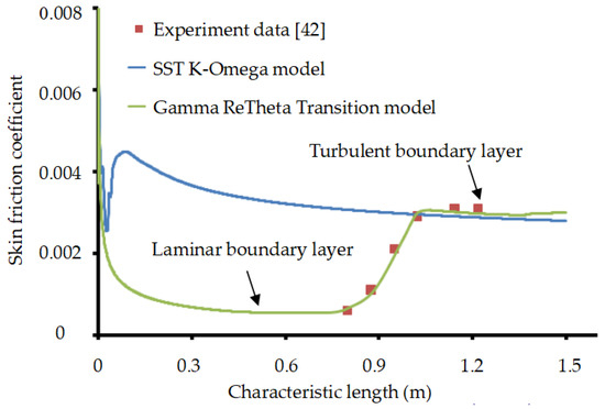
Figure 8.
Validation of the computational setup using the SST K-Omega model.
Figure 9 compares the velocity profiles of the turbulent region obtained by the numerical simulations and experiments [42]. Considering that the parameters in the available literature [42] are in dimensional forms, to facilitate comparison, the x-axis (Y) is not dimensionless in Figure 9. The calculated results show good agreement with the experimental results; thus, the accuracy of the numerical simulations was verified from the perspective of the velocity profile.
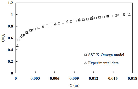
Figure 9.
Mean velocity profiles of physical experiments and simulations.
3.2. Analysis of the Nonsmooth Surface Inspired by Sand Dunes
To study the characteristics of drag reduction, the drag force of the smooth surface and nonsmooth surface were calculated. The drag reduction ratios were defined as follows:
where is the total drag reduction ratio (including pressure drag and skin friction), is the total drag of the model with a smooth surface, is the total drag of the model with a nonsmooth surface, is the skin friction reduction ratio, is the skin friction of the model with a smooth surface, and is the skin friction of the model with a nonsmooth surface.
The results of drag reduction are shown in Table 2, which show that the nonsmooth surface effectively reduced the skin friction with a reduction ratio () of 39.86%. However, the decrease in skin friction was accompanied by a sharp increase in pressure drag, which lead to a net increase in total drag.
Table 2.
Drag reduction ratio of the nonsmooth surface.
As shown in Figure 10, the nonsmooth unit cell changed the wall pressure distribution, and a peak pressure point was formed in the front of the nonsmooth unit cell (windward side). The difference in pressure between the windward side and the slip side constitutes the pressure drag, which eventually leads to a net increase in total drag. The rapid increase in pressure drag is a common problem in designing nonsmooth surfaces [41,51,52,53].
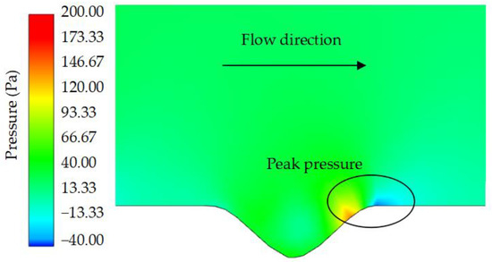
Figure 10.
Pressure contour of the nonsmooth unit cell.
3.3. Analysis of Nonsmooth Surface with a Jet
To solve the drastic increase in the pressure drag of the nonsmooth surface, a new active surface based on a bionic nonsmooth surface with a jet was proposed. The bionic inspiration came from sharks. Previous studies have shown that the jetting mechanism of shark gills has a remarkable drag reduction effect; therefore, the shark gill was adopted as the bionic prototype. Accordingly, the jet hole was set on the leeward side of the nonsmooth unit cell, wherein the jet hole was oriented in the direction of the incoming flow. When the fluid flowed through the active surface, the jet hole injected low-speed fluid.
Figure 11 shows a schematic diagram of the active surface unit. The jet hole was set in the front of the nonsmooth unit cell, whereas the shape of the unit cell remained unchanged. The drag reduction ratios () of the active surface under different jet velocities are shown in Figure 12.
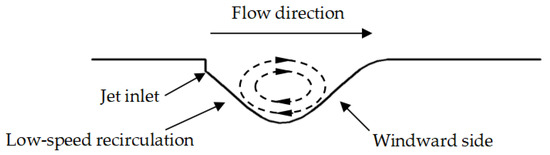
Figure 11.
Schematic diagram of the active surface unit cell.
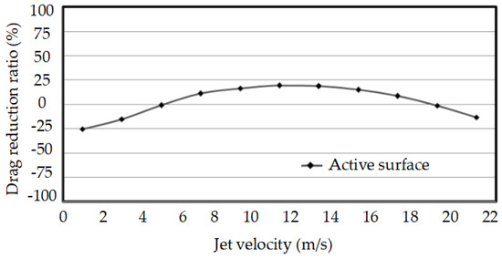
Figure 12.
Drag reduction ratio of the active surface.
The drag reduction effects were different under different jet velocities; however, the total drag on the nonsmooth surface with a jet was lower than that on the nonsmooth surface (). When the jet velocity was between 7 m/s and 17 m/s, the active surface significantly achieved drag reduction effects, and the drag reduction ratio reached a maximum at 19.35% when the jet velocity was set to 11 m/s.
The simulation results also show that the active surface had significant effects on the skin friction reduction. The drag reduction effect of the active surface was better than that of the nonsmooth surface, and the skin friction reduction ratio increased with increasing jet velocity (Figure 13).
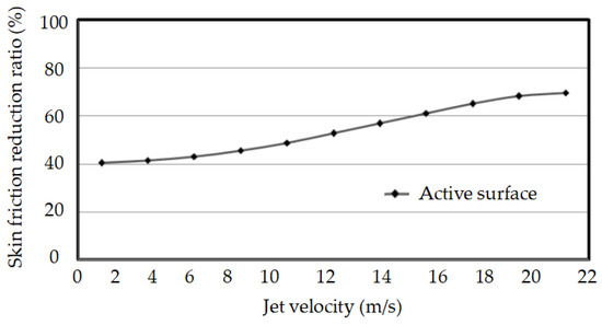
Figure 13.
Skin friction reduction ratio of the active surface.
When the skin friction decreased, the relative increase in pressure drag between the smooth surface to nonsmooth surface decreased. The pressure drag of the active surface was smaller than that of the nonsmooth surface (dotted box in Table 3). However, the active surface could not eliminate the net increase in pressure drag.
Table 3.
Results of numerical simulations.
The drag changes in the outlet section (surface B) are shown in Table 4. The active surface influenced both the area near the nonsmooth unit cell and the distant areas behind the active surface. The drag reduction ratio in this area also increased with increasing jet velocity.
Table 4.
Drag changes of surface B.
3.4. Drag Reduction Mechanism
When the jet velocity reached 11 m/s, the active surface achieved the greatest drag reduction ratio. Therefore, an analysis of the turbulent kinetic energy, pressure distribution, and velocity characteristics at a jet velocity of 11 m/s was carried out to investigate the drag reduction mechanism.
3.4.1. Turbulent Kinetic Energy
The drag reduction behavior was clearly related to the turbulent kinetic energy. Turbulent kinetic energy represents the fluctuation length of turbulence, which can indicate the energy exchange frequency. The larger the turbulent kinetic energy was, the greater the energy loss produced. Figure 14 shows the turbulent kinetic energy contours of three surfaces at .
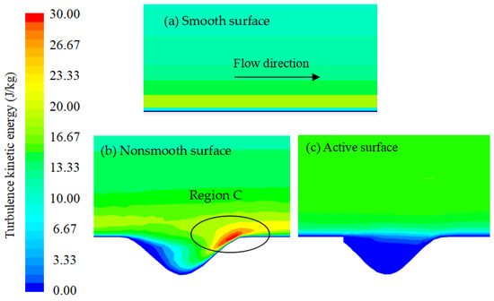
Figure 14.
Kinetic energy contour.
The turbulent kinetic energy intensities of the nonsmooth surface and active surface were obviously less than that of the smooth surface, especially in the nonsmooth unit cell. However, the turbulent kinetic energy intensity on the windward side of the nonsmooth surface was markedly enhanced (region C). The existence of fluid diversion was the main reason for this phenomenon. The improved active surface alleviated the problem of fluid separation and had lower turbulent kinetic energy.
Figure 15 shows the turbulent kinetic energy in the outlet section in surface B, see Figure 4. The turbulent kinetic energy intensity of the active surface was significantly lower than that of the other surfaces. The active surface clearly affected the turbulent kinetic energy in the vicinity of the unit cell and in the downstream areas of the active surface.
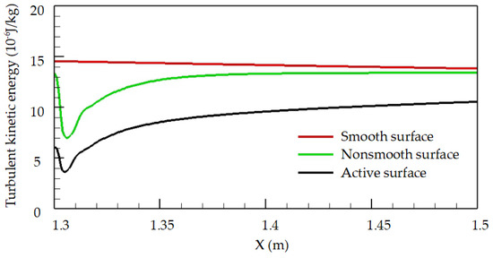
Figure 15.
Comparison of turbulent kinetic energy near wall (surface B).
It is evident from Figure 16 that an obvious closed recirculation region in which the velocity remained very low, was formed within the unit cell, and a mainstream flowed outside this region. The rotational direction at the bottom of the recirculation was opposite to that of the mainstream, whereas the rotational direction on the top was consistent with that of the mainstream.
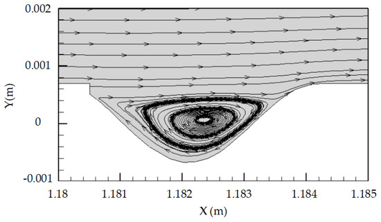
Figure 16.
Recirculation region.
The presence of low-speed recirculation was similar to a rolling bearing. The resistance of rolling friction was less than that of sliding friction under the same conditions. If the friction between the fluid and the fixed wall was defined as fluid–wall sliding friction, then the role of the rolling bearing (recirculation) was to convert the original sliding friction into fluid–fluid rolling friction. The fluid–fluid rolling friction reduced momentum exchange and turbulent kinetic energy, resulting in drag reduction. In addition, the recirculation seemed to relax the no-slip boundary condition, which lead to lower momentum losses in the active surface than in the smooth surface. Thus, the rolling bearing (recirculation) was one of the mechanisms governing the observed drag reduction.
3.4.2. Pressure Distribution
Figure 17a shows the pressure contour of the nonsmooth surface. Static pressure changes occured on the wall due to the existence of the nonsmooth unit cell. A high-pressure zone was formed on the windward side. An abnormal point was also found in the preceding discussion on turbulent kinetic energy at this same location (region C). The main cause of the high-pressure zone was the stagnation of the mainstream flow on the windward side of the unit cell (Figure 18). When the mainstream flow reached the windward side, some fluid continued to move forward, whereas the rest of the fluid entered the unit and formed a recirculation. Thus, the velocity at this position was greatly reduced, and a high pressure area was formed on the windward side. Moreover, the stagnation of the flow also lead to an increase in momentum exchange. This phenomenon was the reason for the increase in turbulent kinetic energy intensity in this area (discussed in Section 3.4.1).
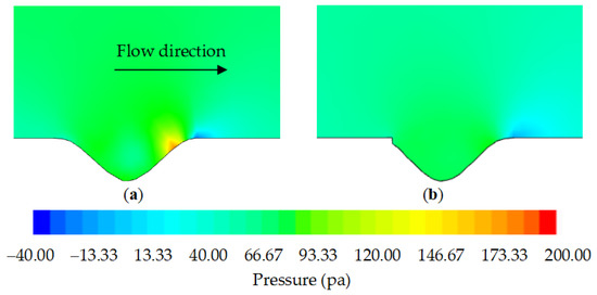
Figure 17.
Pressure contour of proposed surfaces. (a) Nonsmooth surface. (b) Active surface.
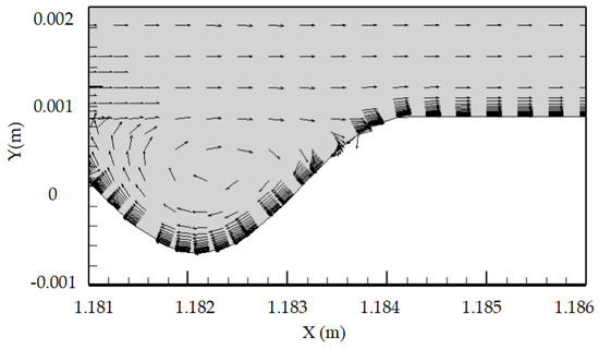
Figure 18.
Vector on the windward side.
When the fluid entered the inner part of the unit cell, a recirculation was formed within the unit cell, and a low-pressure zone was formed on the slip side. The rapid increase in pressure drag on the nonsmooth surface came from the alternating high- and low-pressure regions.
The pressure contour of the active surface is shown in Figure 17b. The pressure concentration on the windward side was effectively alleviated. Instead of depending on the mainstream, the jets supplemented the fluid required for the recirculation formation in the unit cell, which eased the flow stagnation on the windward side and effectively reduced the positive pressure, thereby reducing the pressure drag. Furthermore, the flow stagnation solution also reduced the momentum exchange in the windward region, which reduced the energy loss and the skin friction.
3.4.3. Velocity Characteristics
The viscous fluid effects were mainly reflected in the boundary layer. The changes in the boundary layer thickness of three surfaces when are shown in Figure 19. The thickness of the boundary layer referred to the height perpendicular to the wall from the beginning of the boundary layer wall to the position where the tangential flow velocity along the wall reached 99% of the mainstream velocity. The boundary layer of the active surface was the thickest, followed by that of the nonsmooth surface, and the boundary layer of the smooth surface was the thinnest. An increase in the thickness of the boundary layer resulted in a reduction in the average velocity gradient in the boundary layer, which lead to a decrease in skin friction.
Figure 19.
Changes in the boundary layer thickness.
The mean-velocity profiles of the three surfaces are shown in Figure 20. The results show that in the viscous sublayer or log-law region, the average flow velocities of the nonsmooth and active surfaces were significantly less than that of the smooth surface, thereby leading to a decrease in skin friction. The average flow velocity of the active surface was the smallest, so the drag reduction effect was the most obvious.
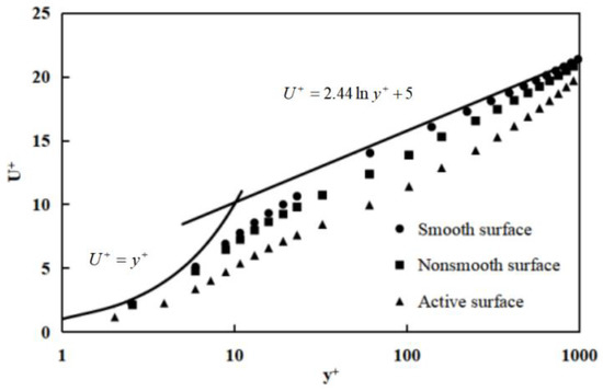
Figure 20.
Changes in mean velocity profiles.
Figure 21 shows the velocities near the wall along the mainstream direction of the three surfaces at the same distance from the wall (δ+ = 0.3, where δ+ is the ratio of the distance from the monitoring point to the wall to the thickness of the boundary layer). The average velocity near the wall with the active surface was lower than that near the wall with the smooth surface and the nonsmooth surface. This trend shows that the flow velocity in the boundary layer decreased when utilizing the nonsmooth surface with a jet, which was equivalent to increasing the thickness of the boundary layer. Furthermore, these findings are consistent with the conclusions drawn above.
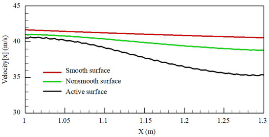
Figure 21.
Comparison of x-velocities near wall.
4. Conclusions
A kind of new active surface was proposed that combines a bionic nonsmooth surface with a jet to achieve drag reduction effects. First of all, a new nonsmooth surface inspired by sand dunes was proposed. The nonsmooth surface can effectively reduce the skin friction, and the maximum skin friction reduction ratio reached 39.86%. However, the decrease in skin friction was accompanied by a sharp increase in pressure drag. An active surface that combines a bionic nonsmooth surface with a jet was then proposed. The active surface overcame the sharp increase of pressure drag and the maximum drag reduction ratio reached 19.35% when the jet velocity was 11 m/s. The main conclusions of this study are as follows:
(1) When fluid flowed through the nonsmooth unit cell, a low-speed recirculation formed within the unit cell. The recirculation transformed the original fluid–wall sliding friction into the fluid–fluid rolling friction, effectively reducing the skin friction. However, due to fluid separation on the windward side, a high-pressure zone formed, leading to a sharp increase in pressure drag.
(2) The active surface generated a low-speed recirculation within the nonsmooth unit cell by jetting low-speed fluid, which effectively reduced the skin friction and the pressure drag caused by flow separation, leading to a reduction in the total drag. The maximum drag reduction ratio with this active surface reached 19.35%, which is better than the commonly accepted drag reduction ratio achieved with grooves (10%).
Author Contributions
X.S. and M.Z. conceived and designed the research topic; X.S. put forward the research method and verified the results; M.Z. performed the numerical analysis.
Funding
This research is funded by the National Natural Science Foundation of China under Grant No. 51375439 and the Science Fund for Creative Research Groups of the National Natural Science Foundation of China under Grant No.51821093.
Conflicts of Interest
The authors declare no conflict of interest.
References
- Verschoof, R.A.; Van der veen, R.C.A.; Sun, C.; Lohse, D. Bubble drag reduction requires large bubbles. Phys. Rev. Lett. 2016, 117, 104502. [Google Scholar] [CrossRef] [PubMed]
- Goyne, C.P.; Stalker, R.J.; Paull, A. Skin-friction measurements in high-enthalpy hypersonic boundary layers. J. Fluid Mech. 2003, 485, 1–32. [Google Scholar] [CrossRef]
- Fan, Y.T.; Cheng, C.; Li, W.P. Effects of the Reynolds number on the mean skin friction decomposition in turbulent channel flows. J. Appl. Math. Mech. (English Edition) 2019, 40, 29–40. [Google Scholar] [CrossRef]
- Rastegari, A.; Akhavan, R. On the mechanism of turbulent drag reduction with super-hydrophobic surfaces. J. Fluid Mech. 2015, 773, R4. [Google Scholar] [CrossRef]
- Glen, M.H.; Newton, M.I.; Shirtcliffe, N.J. Immersed superhydrophobic surfaces: Gas exchange, slip and drag reduction properties. Soft Matter. 2010, 6, 714–719. [Google Scholar]
- Guan, X.L.; Yao, S.Y.; Jiang, N. A study on coherent structures and drag-reduction in the wall turbulence with polymer additives by TRPIV. Acta Mech. Sin. 2013, 29, 485–493. [Google Scholar] [CrossRef]
- Li, F.; Zhao, G.; Liu, W.X.; Sun, Z.Z. Simulation on flow control and drag reduction with bionic jet surface. J. Basic Sci. Eng. 2014, 22, 574–583. [Google Scholar]
- Wang, C.; Tang, H. Enhancement of aerodynamic performance of a heaving airfoil using synthetic-jet based active flow control. Bioinspiration Biomim. 2018, 13, 046005. [Google Scholar] [CrossRef]
- Pang, J.; Choi, K.S. Turbulent drag reduction by Lorentz force oscillation. Phys. Fluids 2004, 16, 35–38. [Google Scholar] [CrossRef]
- Walsh, M.J. Riblets as a viscous drag reduction technique. AIAA Pap. 1983, 21, 485–486. [Google Scholar] [CrossRef]
- Bechert, D.W.; Bruse, M.; Hage, W. Experiments on drag-reducing surfaces and their optimization with an adjustable geometry. J. Fluid Mech. 1997, 338, 59–87. [Google Scholar] [CrossRef]
- Martin, S.; Bhushan, B. Fluid flow analysis of a shark-inspired microstructure. J. Fluid Mech. 2014, 756, 5–29. [Google Scholar] [CrossRef]
- Chamorro, L.P.; Arndt, R.E.A.; Sotiropoulos, F. Drag reduction of large wind turbine blades through riblets: Evaluation of riblet geometry and application strategies. Renew. Energy 2013, 50, 1095–1105. [Google Scholar] [CrossRef]
- Yang, S.Q.; Tian, H.P.; Wang, Q.Y.; Jiang, N. Tomographic PIV investigation on coherent vortex structures over shark-skin inspired drag-reducing riblets. Acta Mech. Sin. 2016, 32, 284–294. [Google Scholar] [CrossRef]
- Sasamori, M.; Lihama, O.; Mamori, H.; Lwamoto, K.; Murata, A. Parametric study on a sinusoidal riblet for drag reduction by direct numerical simulation. Flow Turbul. Combust. 2017, 99, 47–69. [Google Scholar] [CrossRef]
- Huang, C.; Liu, D.; Wei, J. Direct numerical simulation of surfactant solution flow in the wide-rib rectangular grooved channel. AIChE J. 2018, 64, 2898–2912. [Google Scholar] [CrossRef]
- Garcia-Mayprai, R.; Jimenez, J. Hydrodynamic stability and breakdown of the viscous regime over riblets. J. Fluid Mech. 2011, 678, 317–347. [Google Scholar] [CrossRef]
- Klumpp, S.; Meinke, M.; Schroder, W. Numerical simulation of riblet controlled spatial transition in a zero-pressure-gradient boundary layer. Flow Turbul. Combust. 2010, 85, 57–71. [Google Scholar] [CrossRef]
- Choi, C.H.; Ulmanella, U.; Kim, J. Effective slip and friction reduction in nanograted superhydrophobic microchannels. Phys. Fluids 2006, 18, 781–782. [Google Scholar] [CrossRef]
- Koch, K.; Bhushan, B.; Barthlott, W. Multifunctional surface structures of plants: An inspiration for biomimetics. Prog. Mater. Sci. 2009, 54, 137–178. [Google Scholar] [CrossRef]
- Liu, K.; Tian, Y.; Jiang, L. Bio-inspired superdrophobic and smart materials: Design, fabrication, and application. Prog. Mater. Sci. 2013, 58, 503–564. [Google Scholar] [CrossRef]
- Daniello, R.J.; Waterhouse, N.E.; Rothstein, J.P. Drag reduction in turbulent flows over superhydrophobic surfaces. Phys. Fluids 2009, 21, 085103. [Google Scholar] [CrossRef]
- Rastegari, A.; Akhavan, R. The common mechanism of turbulent skin-friction drag reduction with superhydrophobic longitudinal microgrooves and riblets. J. Fluid Mech. 2018, 838, 68–104. [Google Scholar] [CrossRef]
- Min, T.; Kim, J. Effects of hydrophobic surface on skin-friction drag. Phys. Fluids 2004, 16, L55. [Google Scholar] [CrossRef]
- Martell, M.B.; Perot, J.B.; Rothstein, J.P. Direct numerical simulations of turbulent flows over superhydrophobic surfaces. J. Fluid Mech. 2009, 620, 31–41. [Google Scholar] [CrossRef]
- Ou, J.; Perot, B.; Rothstein, J.P. Laminar drag reduction in microchannels using ultrahydrophobic surfaces. Phys. Fluids 2004, 16, 4635–4643. [Google Scholar] [CrossRef]
- Ou, J.; Rothstein, J.P. Direct velocity measurements of the flow past drag-reducing ultrahydrophobic surfaces. Phys. Fluids 2005, 17, 103606. [Google Scholar] [CrossRef]
- Costantini, R.; Mollicone, J.P.; Battista, F. Drag reduction induced by superhydrophobic surfaces in turbulent pipe flow. Phys. Fluids 2018, 30, 025102. [Google Scholar] [CrossRef]
- Park, H.; Park, H.; Kim, J. A numerical study of the effects of superhydrophobic surface on skin-friction drag in turbulent channel flow. Phys. Fluids 2013, 25, 110815. [Google Scholar] [CrossRef]
- Herrmann, H.J.; Sauermann, G. Shape of dunes. Physic A Stat. Mech. Its Appl. 2000, 283, 24–30. [Google Scholar] [CrossRef]
- Hesp, P.A.; Hastings, K. Width, height and slope relationships and aerodynamic maintenance of barchans. Geomorphology 1998, 22, 193–204. [Google Scholar] [CrossRef]
- Weng, W.S.; Hunt, J.C.R.; Carruthers, D.J. Air flow and sand transport over sand-dunes. Acta Mech. 1991, 2, 1–22. [Google Scholar]
- Gao, G.; Ning, H. Theoretical and experimental study in stability of the barchan dune vortex flame. J. Eng. 1982, 3, 89–95. [Google Scholar]
- Li, K.; Zeng, Z.X.; Xu, Y.H. Research of leeward angle of a new dune-shaped dump combustor. J. Proj. Rocket. Missiles Guid. 2014, 34, 99–102. [Google Scholar]
- Tao, W.Q.; Sparrow, E.M. The transportive property and convective numerical stability of the steady-state convection-diffusion finite-difference equation. Numer. Heat Transf. 1987, 11, 491–497. [Google Scholar] [CrossRef]
- Lighthill, M.J. Hydromechanics of aquatic animal propulsion. Annu. Rev. Fluid Mech. 1969, 1, 413–416. [Google Scholar] [CrossRef]
- Babenko, V.V.; Koval, A.P. Hydrodynamic functions of swordfish gill system. Bionika 1982, 16, 11–15. [Google Scholar]
- Li, F.; Zhao, G.; Liu, W.X. Numerical simulation and experimental study on drag reduction performance of bionic jet hole shape. Acta Phys. Sin. 2015, 64, 1–8. [Google Scholar]
- Zhang, G.; Gu, Y.Q.; Xu, G.Y. Experimental study on drag reduction characteristics of bionic jet surface. J. Cent. South Univ. (Sci. Technol.) 2012, 43, 3007–3012. [Google Scholar]
- Claudin, P.; Wiggs, G.F.S.; Andreotti, B. Field evidence for the upwind velocity shift at the crest of low dunes. Bound.-Layer Meteorol. 2013, 148, 195–206. [Google Scholar] [CrossRef]
- Song, X.W.; Zhang, M.X.; Lin, P.Z. Skin friction reduction characteristics of nonsmooth surfaces inspired by the shapes of barchan dunes. Math. Probl. Eng. 2017, 2017, 6212605. [Google Scholar] [CrossRef]
- Schubauer, G.B.; Klebanoff, P.S. Contributions on the mechanics of boundary-layer transition. Tech. Rep. Arch. Image Libr. 1956, 39, 411–415. [Google Scholar]
- Menter, F.R. Two-equation eddy-viscosity turbulence modeling for engineering applications. AIAA J. 1994, 32, 1598–1605. [Google Scholar] [CrossRef]
- Hellsten, A. Some improvements in Menter’s k-omega SST turbulence model. AIAA J. 1998, 2554, 1–11. [Google Scholar]
- Liu, Y.W.; Yan, H.; Fang, L. Modified k-ω model using kinematic vorticity for corner separation in compressor cascades. Sci. China Technol. Sci. 2016, 59, 795–806. [Google Scholar] [CrossRef]
- John, V.P.; Kuldeep, S. The numerical simulation of a staged transverse injection behind a rearward facing step into a mach 2 stream in a confined environment. Int. J. Eng. Res. Dev. 2012, 4, 54–61. [Google Scholar]
- Patankar, S.V. Numerical Heat Transfer and Fluid Flow; Taylor & Francis: New York, NY, USA, 1980; pp. 25–39. [Google Scholar]
- Shih, T.M. Numerical Heat Transfer; Springer: Berlin/Heidelberg, Germany, 1984; pp. 30–36. [Google Scholar]
- Ni, M.J.; Tao, W.Q. Stability analysis for discretized steady convective-diffusion equation. Numer. Heat Transf. Part B Fundam. 1999, 35, 369–388. [Google Scholar]
- Ni, M.J.; Tao, W.Q.; Wang, S.J. Stability-controllable second-order difference scheme for convection term. J. Therm. Sci. 1998, 7, 119–130. [Google Scholar] [CrossRef]
- Bearman, P.W.; Harvey, J.K. Control of circular cylinder flow by the use of dimples. AIAA J. 1993, 31, 1753–1756. [Google Scholar] [CrossRef]
- Lienhart, H.; Breuer, M.; KoKsoy, C. Drag reduction by dimples-a complementary experimental/numerical investigation. Int. J. Heat Fluid Flow 2008, 29, 783–791. [Google Scholar] [CrossRef]
- Fu, Y.F.; Yuan, C.Q.; Bai, X.Q. Marine drag reduction of shark skin inspired riblet surfaces. Biosurface Biotribology 2017, 3, 11–24. [Google Scholar] [CrossRef]


© 2019 by the authors. Licensee MDPI, Basel, Switzerland. This article is an open access article distributed under the terms and conditions of the Creative Commons Attribution (CC BY) license (http://creativecommons.org/licenses/by/4.0/).