Numerical Analysis on Flexural Behavior of Steel Fiber-Reinforced LWAC Beams Reinforced with GFRP Bars


Abstract
:
1. Introduction
2. Nonlinear Finite–Element Modeling
2.1. General
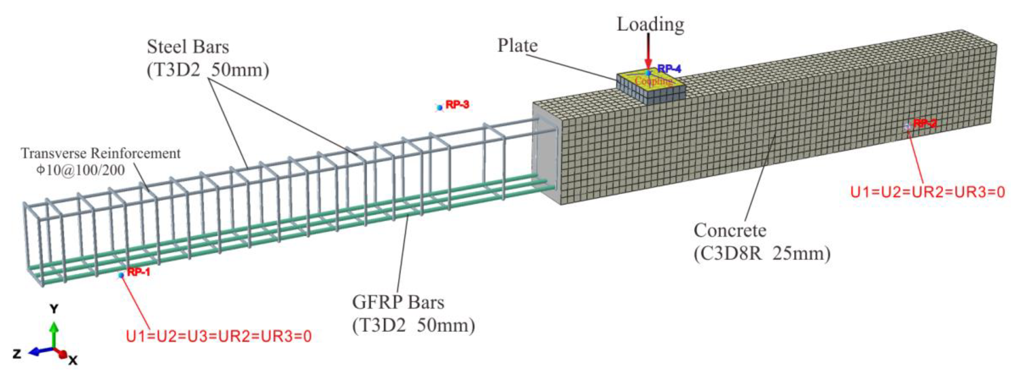
2.2. Finite-Element Geometry and Mesh
2.3. Boundary Conditions and Load Application
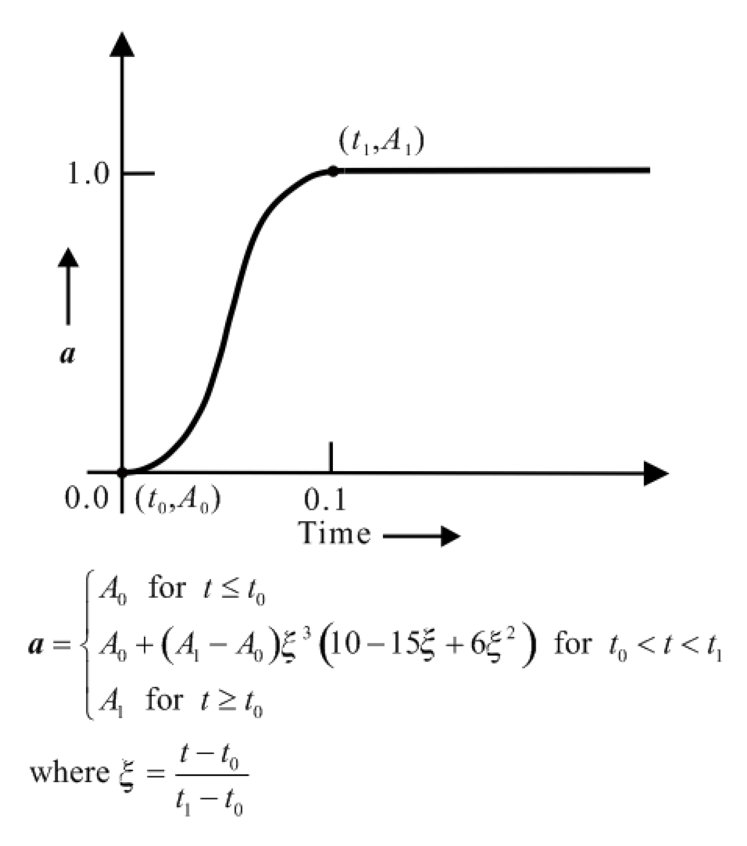
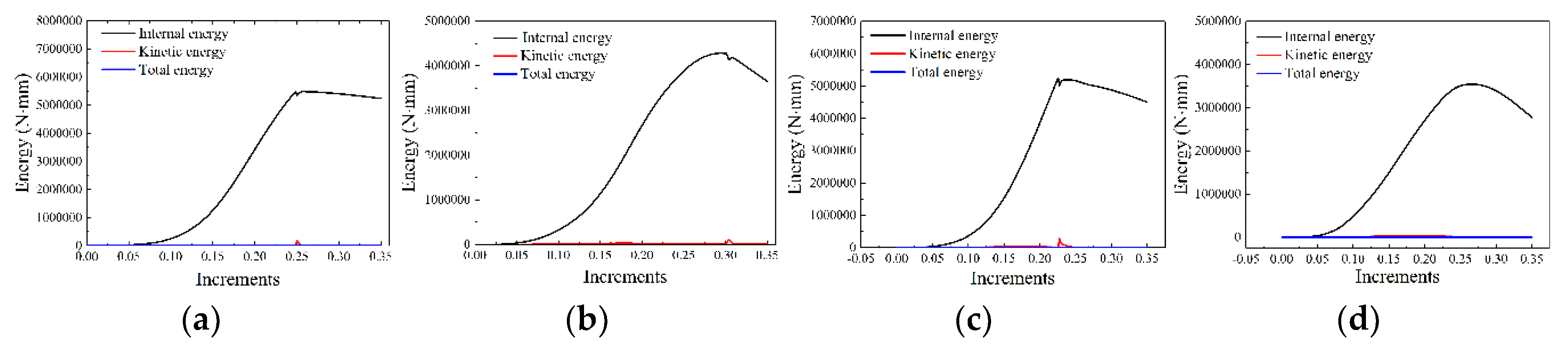
2.4. Dynamic Explicit Solution Scheme
2.5. Material Model
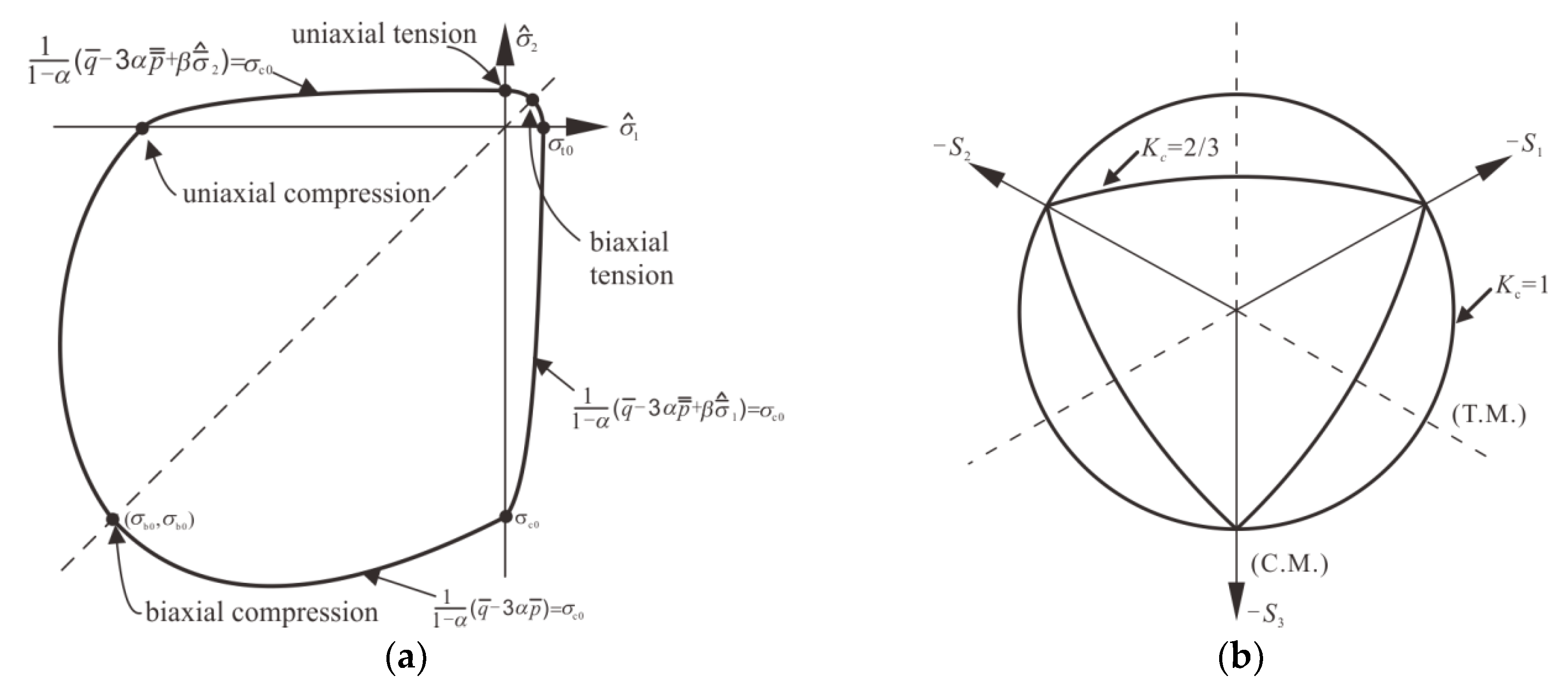
2.5.1. CDP Model
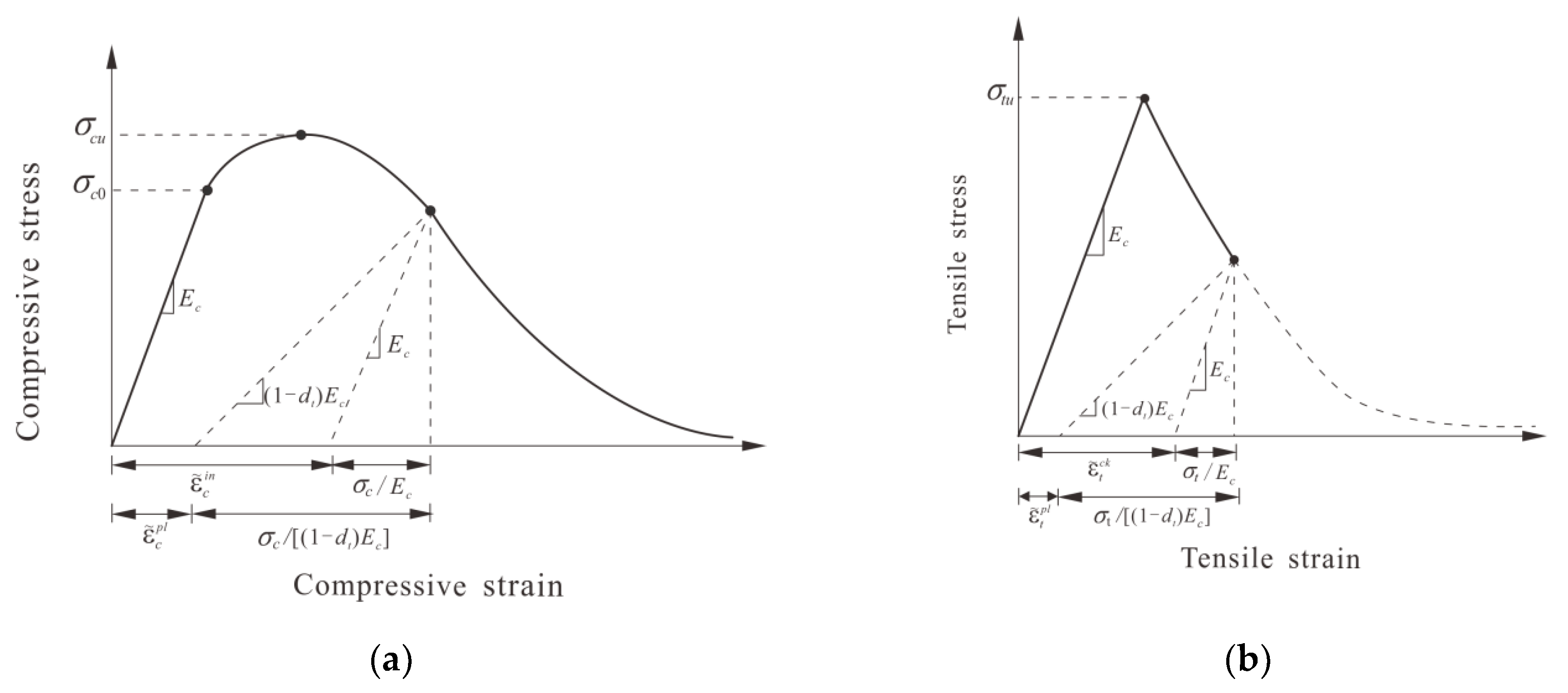
2.5.2. Compressive Stress–Strain Relationship
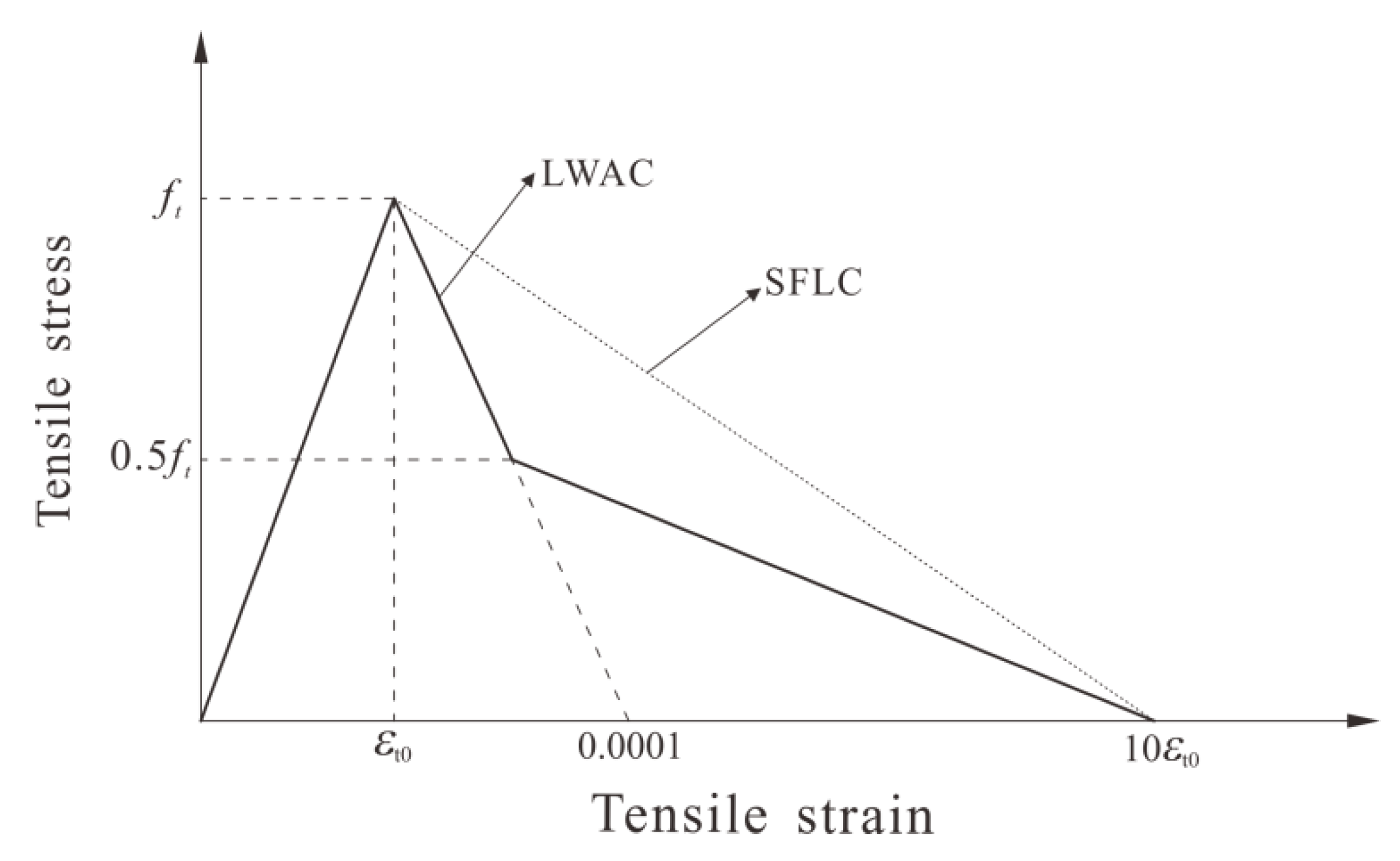
2.5.3. Tensile Behavior
2.5.4. Damage Evolution
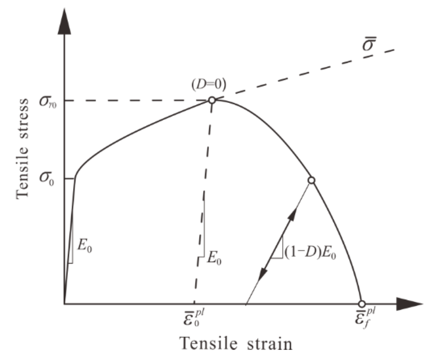
2.5.5. Modeling of GFRP and Steel Bars
3. Experimental Tests
3.1. Material and Specimens
3.2. Test Results
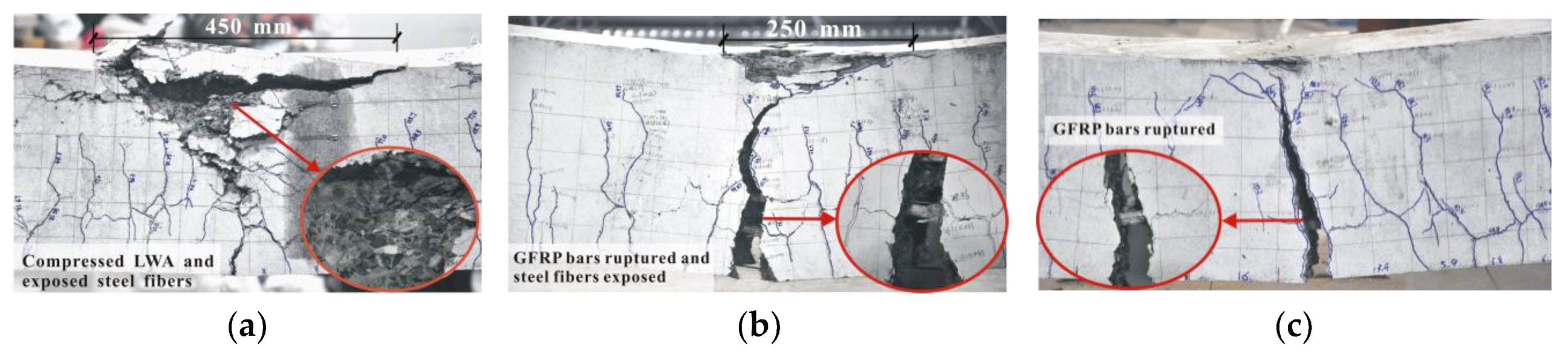
3.2.1. Failure Mode
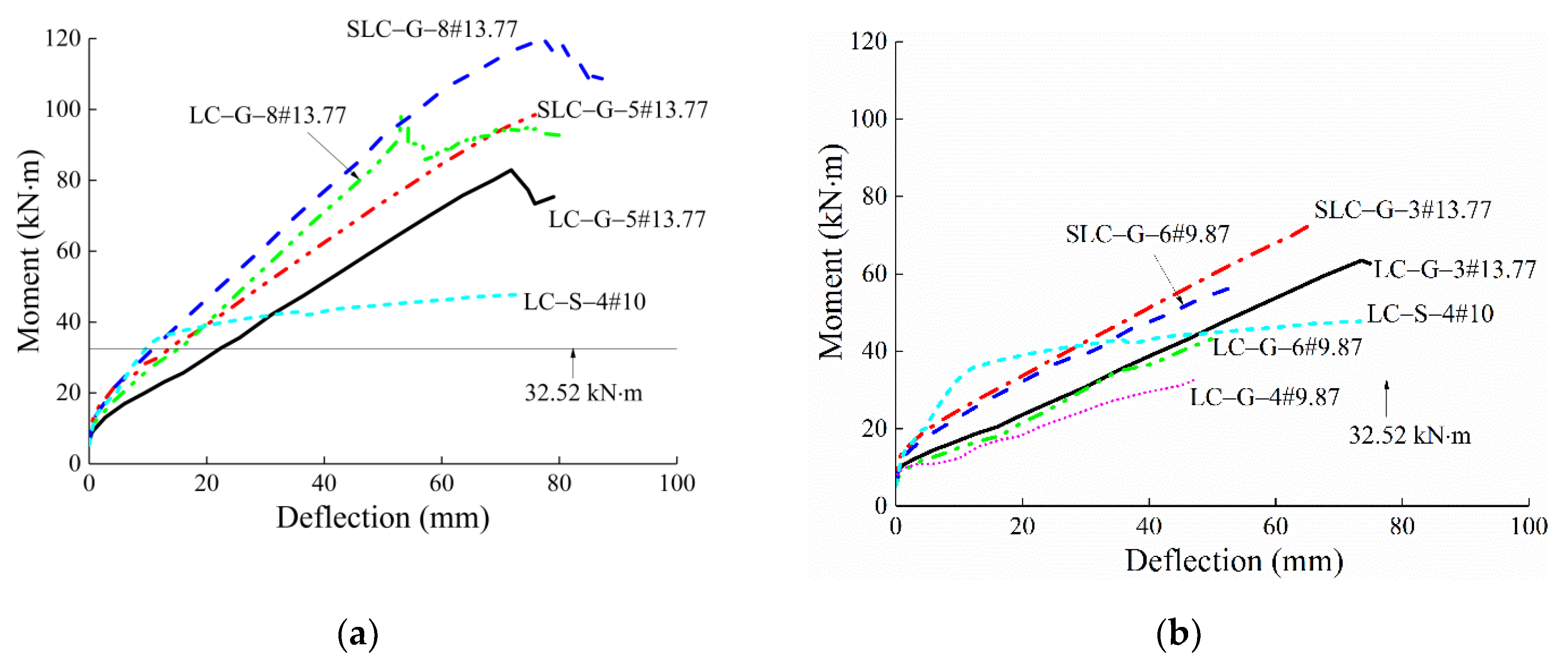
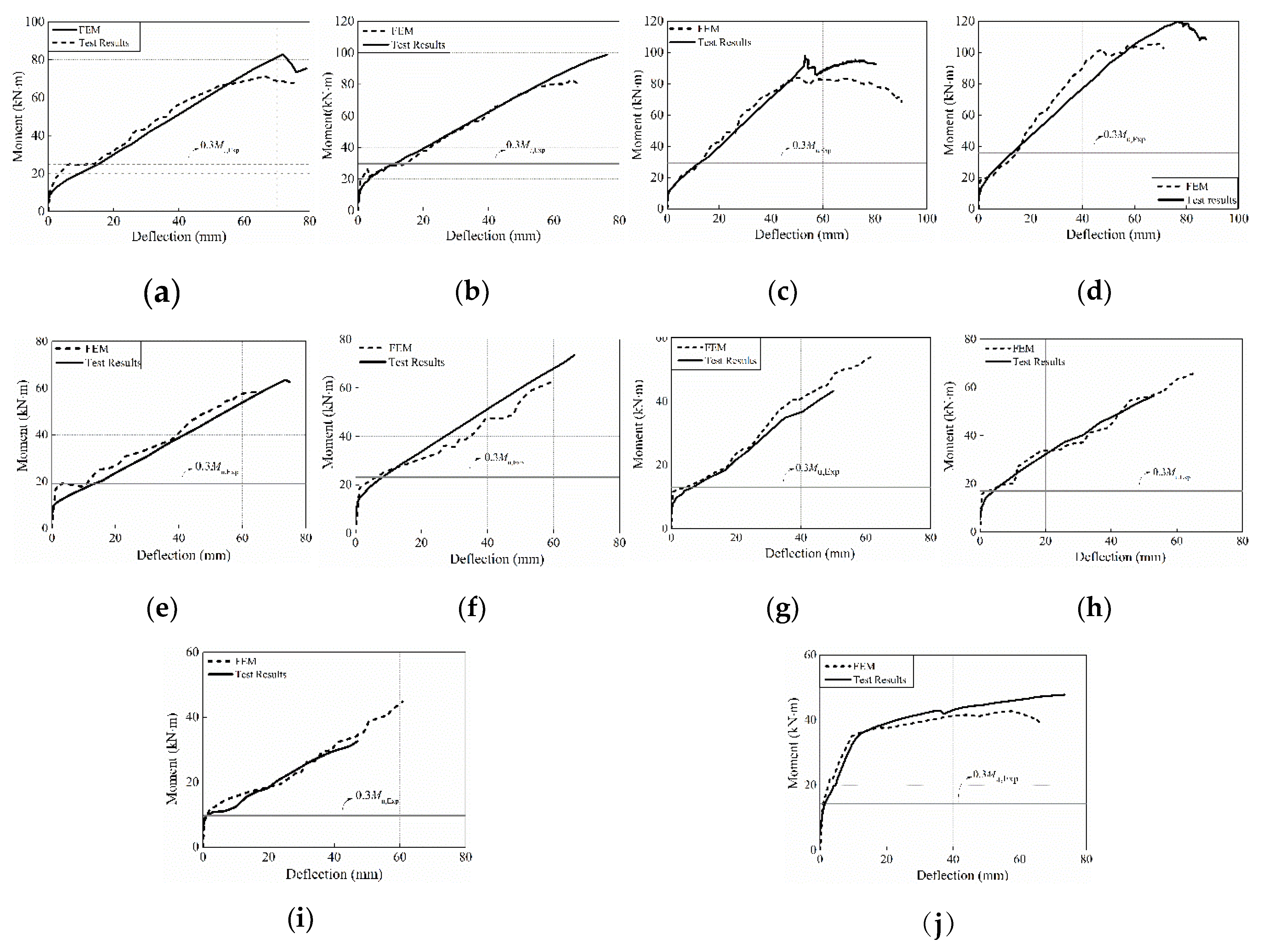
3.2.2. Moment–Deflection Relationship
3.2.3. Deflection at Service Load
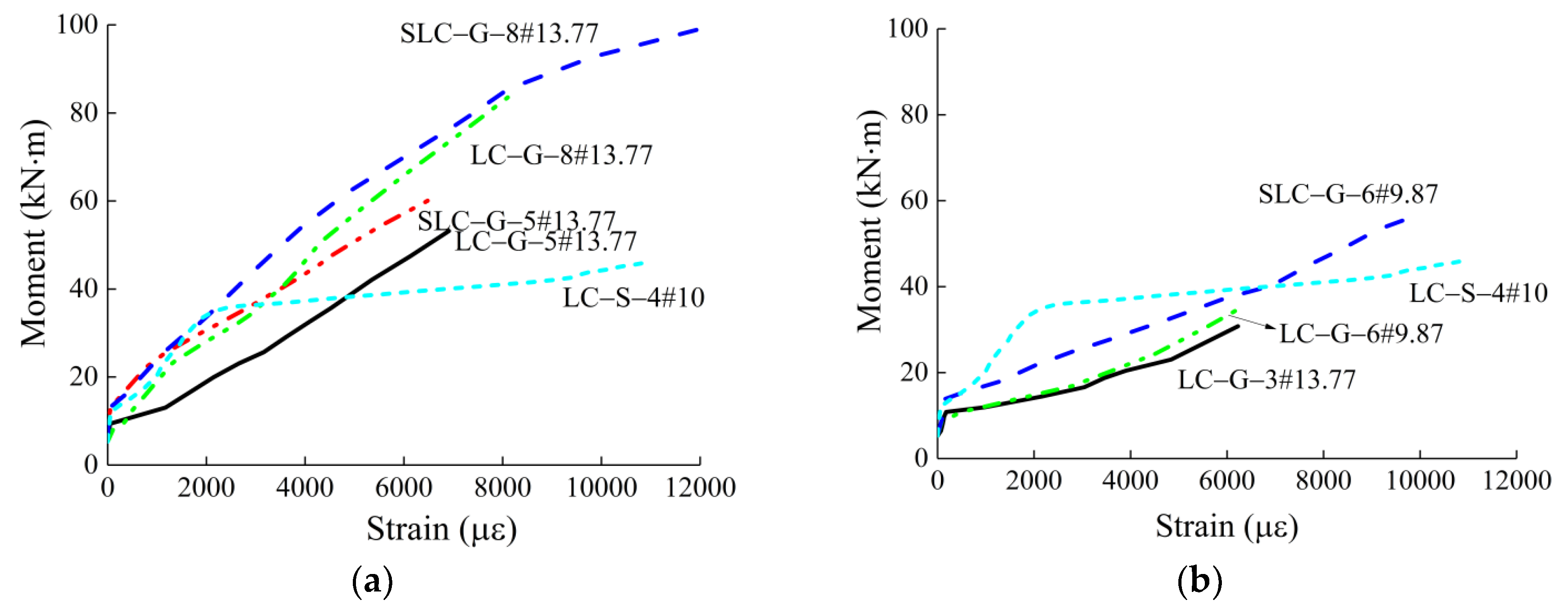
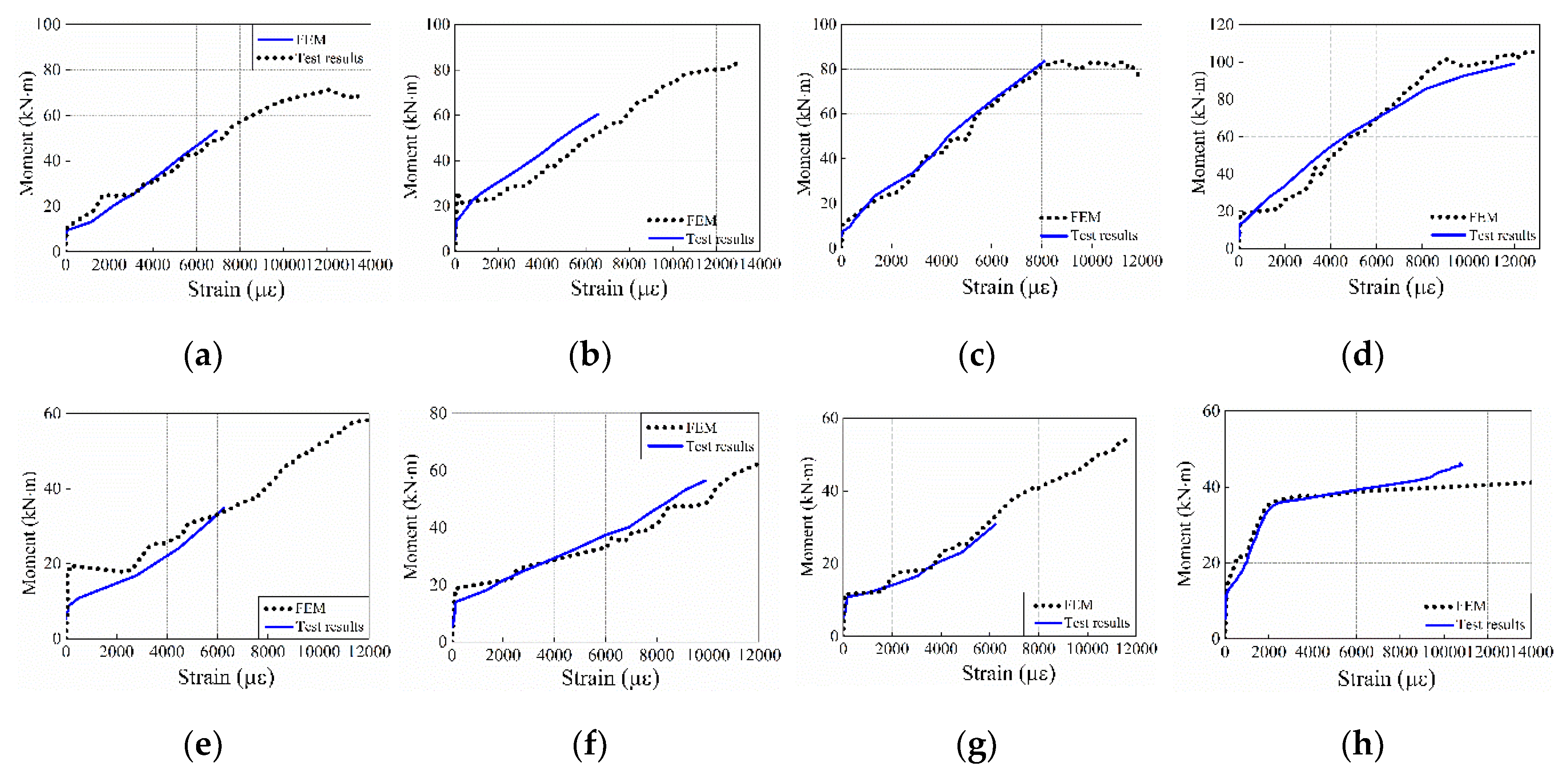
3.2.4. Moment–FRP Strain Relationship
4. Validation of the Established FE Models
4.1. Failure Mode and Crack Pattern
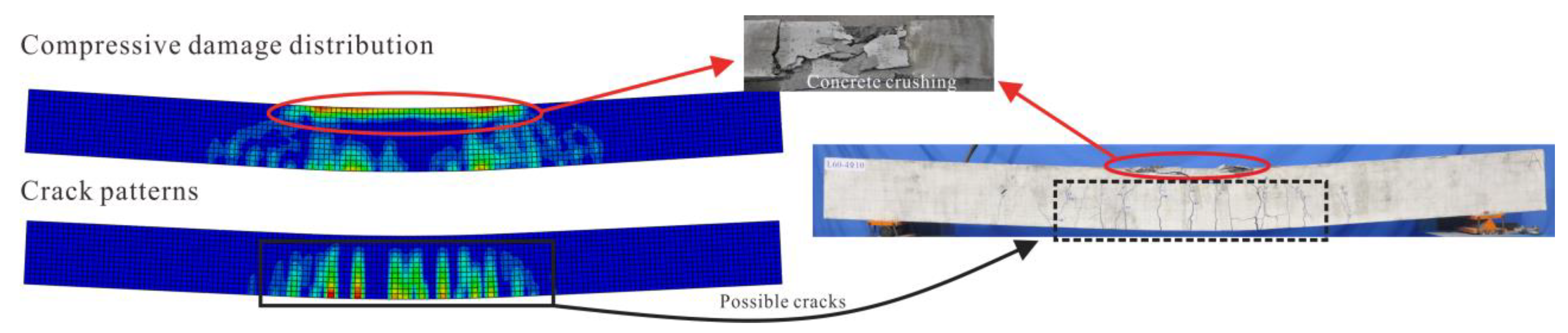
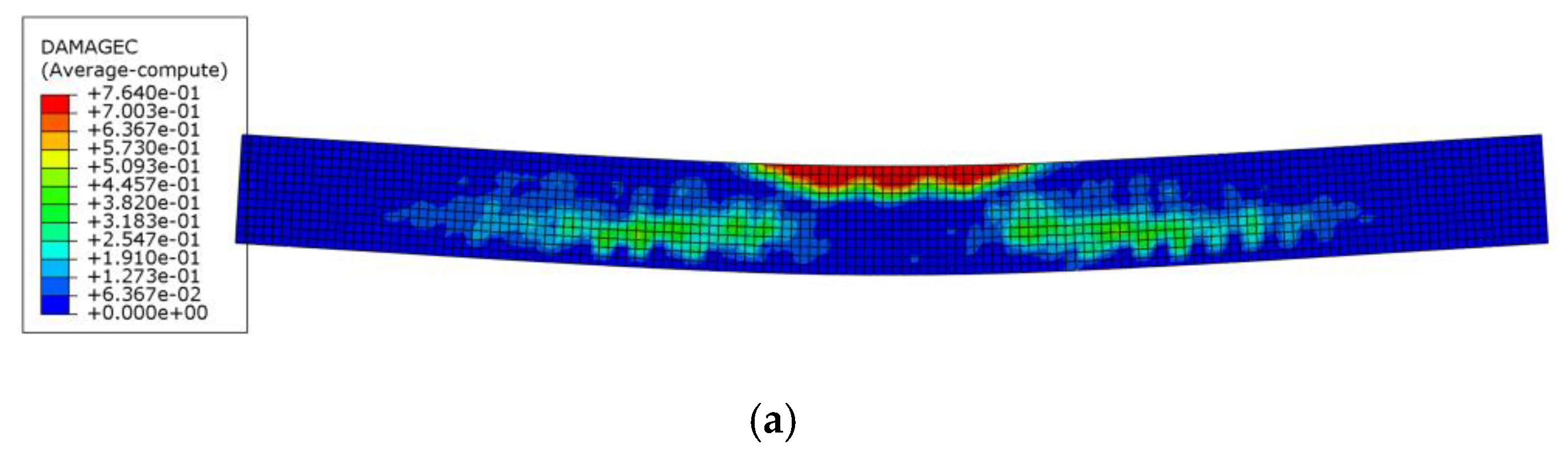
4.1.1. Concrete Crushing for Steel Reinforced Beam
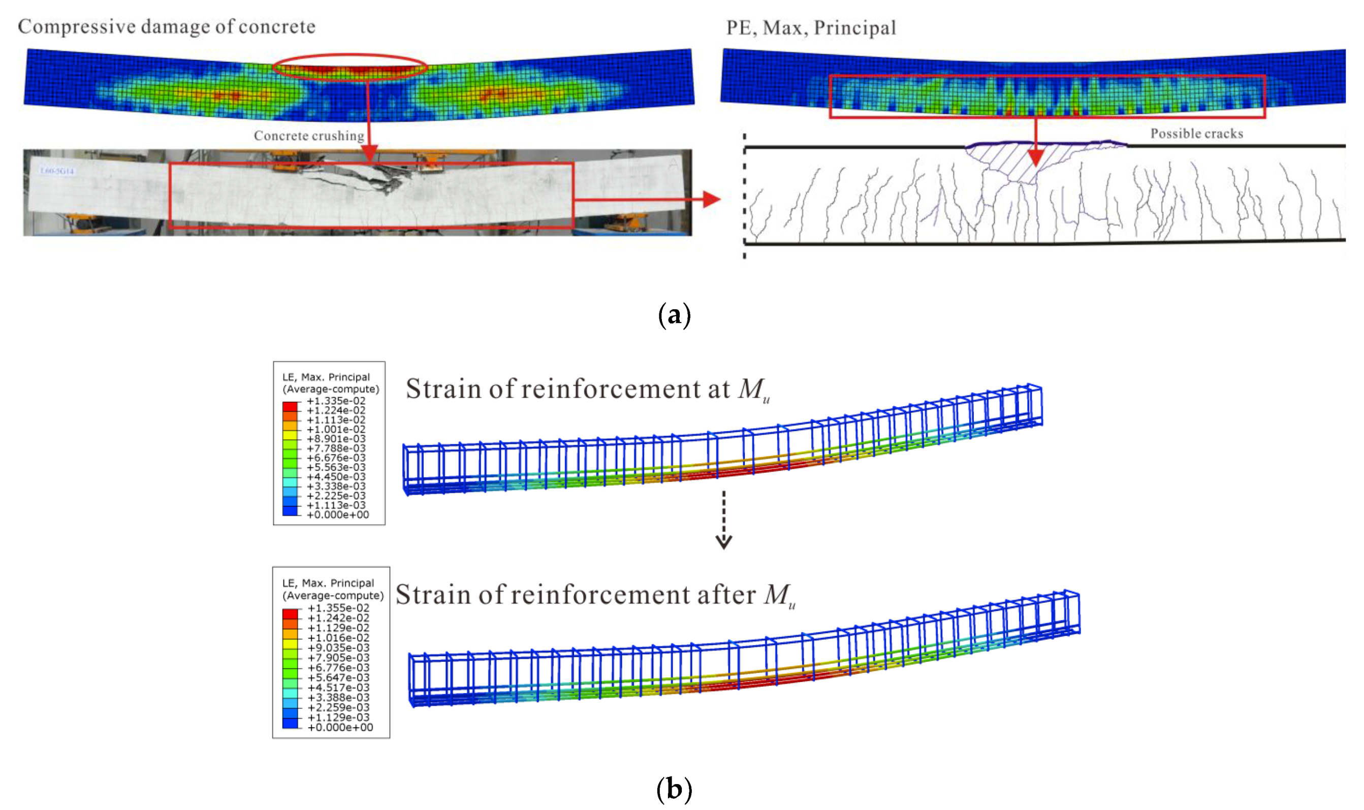
4.1.2. Concrete Crushing for GFRP-Reinforced Beam
4.1.3. Balanced Failure
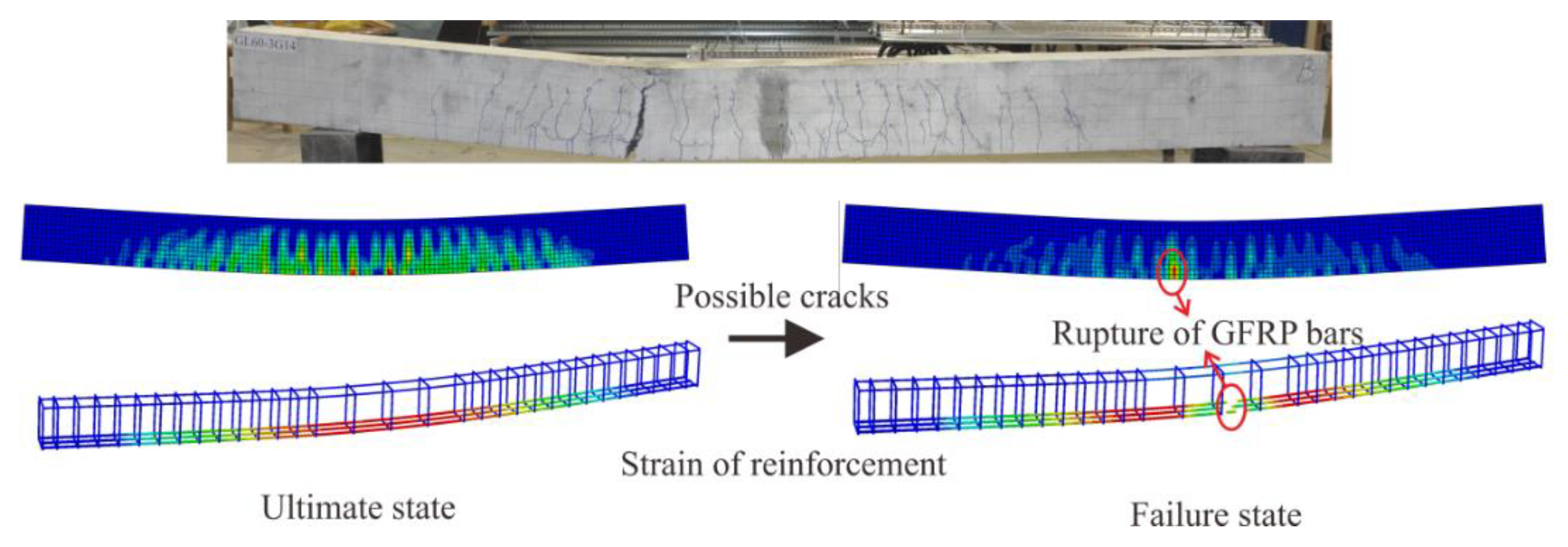
4.1.4. FRP Rupture
4.2. Deflection Behavior, Ultimate Capacity, and FRP Strain
5. Parametric Analysis
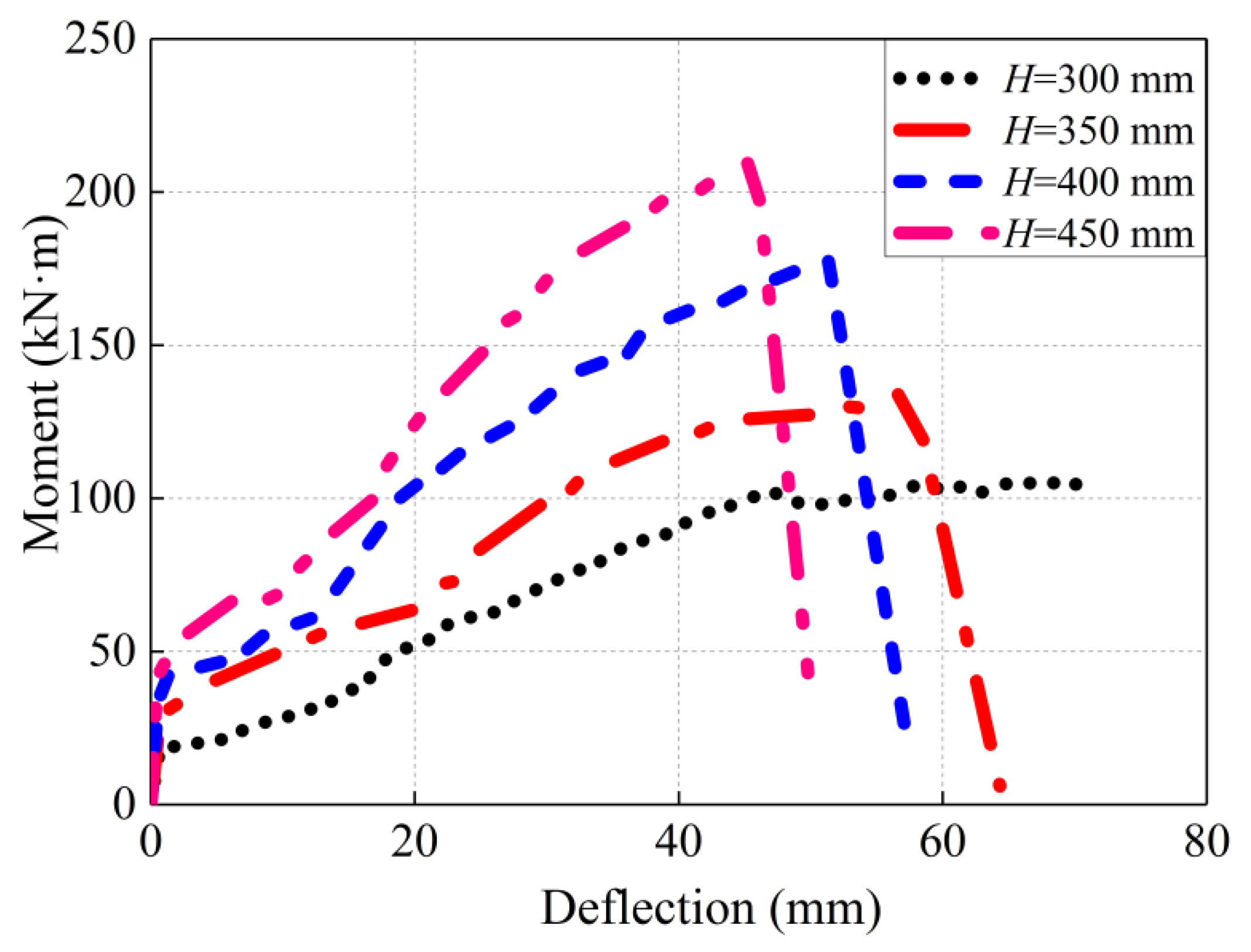
5.1. Section Height
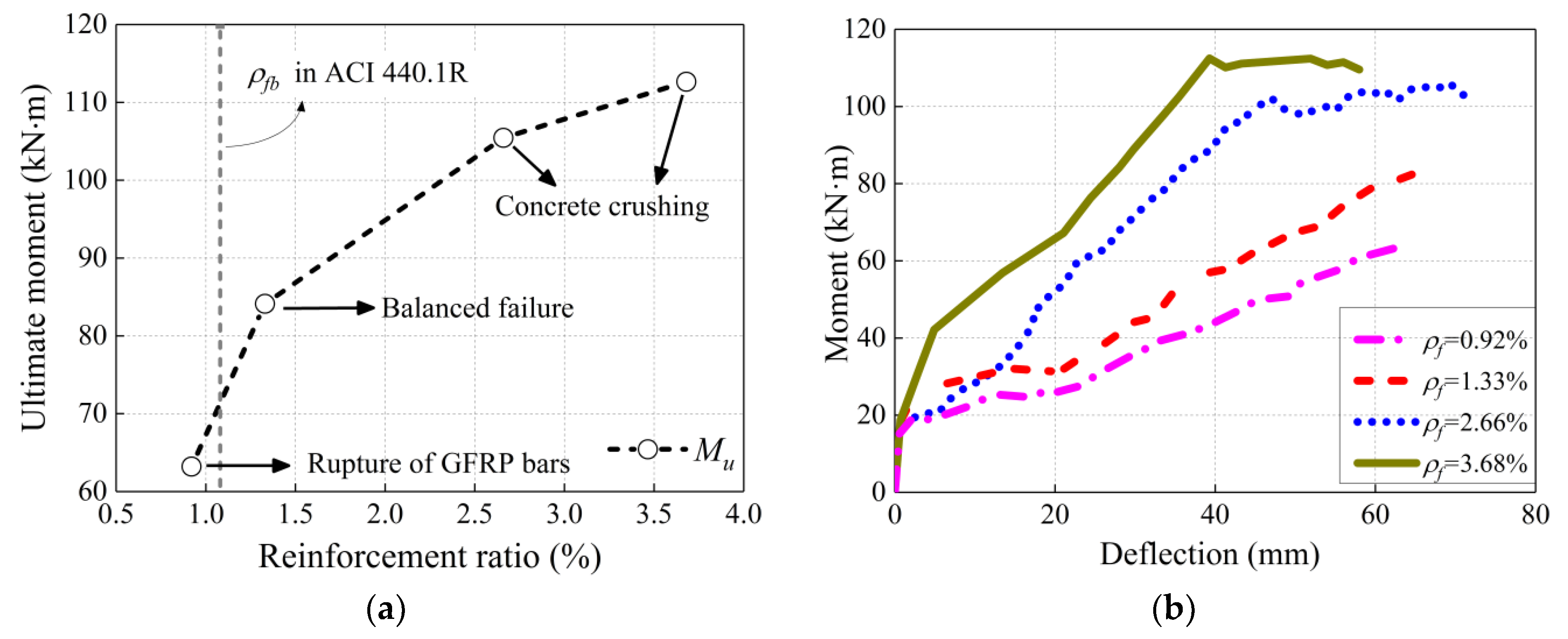
5.2. Reinforcement Ratio
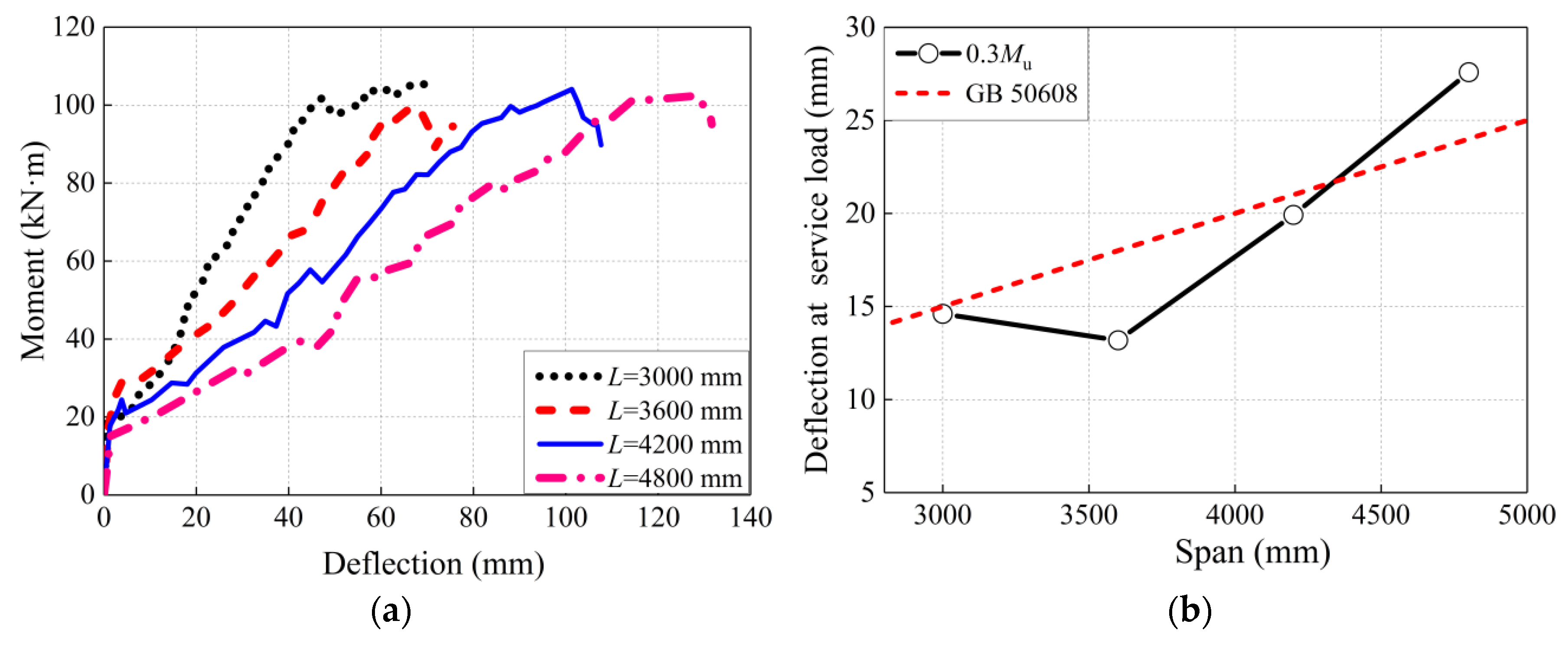
5.3. Length of Span L
6. Conclusions
- (1)
- The established FE models successfully obtained three failure modes of beams referring to the test results, namely concrete crushing, balanced failure, and FRP rupture. This confirmed that the constitutive models of LWAC and SFLC introduced in the FE model are efficient, and the inclusion of progressive damage into the properties of GFRP bars is capable of reflecting the rupture behavior. Moreover, the explicit procedure entails the uninterrupted calculation when brittle failures occurred.
- (2)
- The FE models yielded accurate ultimate capacity predictions with an average experimental-to-predicted ratio of 1.04 ± 0.17. At service load, the estimated deflection closely matched the measured results with an average experimental-to-predicted ratio of 1.09 ± 0.19.
- (3)
- The reinforcement ratio corresponding to balanced failure was higher than that given by code ACI 440.1R, which confirmed the necessity of the amplification factor of a balanced reinforcement ratio to ensure the concrete crushing of the beam.
- (4)
- For specimens that failed due to concrete crushing, the increase in the FRP reinforcement ratio did not significantly improve the ultimate capacity, but it did have an obvious effect on the reduction of deflection at service load.
- (5)
- The increase rate of the deflection at service load was higher for GFRP-reinforced beams with larger clear span lengths. Therefore, a greater reinforcement ratio is needed for beams when the span length is increased.
Author Contributions
Funding
Conflicts of Interest
References
- Gao, Y.L.; Chao, Z. Experimental study on segregation resistance of nanoSiO2 fly ash lightweight aggregate concrete. Constr. Build. Mater. 2015, 93, 64–69. [Google Scholar] [CrossRef]
- Sohel, K.M.A.; Al-Jabri, K.; Zhang, M.H.; Liew, J.Y.R. Flexural fatigue behavior of ultra-lightweight cement composite and high strength lightweight aggregate concrete. Constr. Build. Mater. 2018, 173, 90–100. [Google Scholar] [CrossRef]
- Gao, J.M.; Wei, S.; Keiji, M. Mechanical properties of steel fiber-reinforced, high-strength, lightweight concrete. Cem. Concr. Compos. 1997, 19, 307–313. [Google Scholar] [CrossRef]
- Karayannis, C.G. Nonlinear analysis and tests of steel-fiber concrete beams in torsion. Struct. Eng. Mech. 2000, 9, 323–338. [Google Scholar] [CrossRef]
- Campione, G. Flexural and shear resistance of steel fiber–reinforced lightweight concrete beams. J. Struct. Eng. 2013, 140, 04013103. [Google Scholar] [CrossRef]
- Grabois, T.M.; Guilherme, C.C.; Toledo Filho, R.D. Fresh and hardened-state properties of self-compacting lightweight concrete reinforced with steel fibers. Constr. Build. Mater. 2016, 104, 284–292. [Google Scholar] [CrossRef]
- Li, J.J.; Wan, C.J.; Niu, J.G.; Wu, L.F.; Wu, Y.C. Investigation on flexural toughness evaluation method of steel fiber reinforced lightweight aggregate concrete. Constr. Build. Mater. 2017, 131, 449–458. [Google Scholar] [CrossRef]
- Libre, N.A.; Shekarchi, M.; Mahoutian, M.; Soroushian, P. Mechanical properties of hybrid fiber reinforced lightweight aggregate concrete made with natural pumice. Constr. Build. Mater. 2011, 25, 2458–2464. [Google Scholar] [CrossRef]
- Blaznov, A.N.; Krasnova, A.S.; Krasnov, A.A.; Zhurkovsky, M.E. Geometric and mechanical characterization of ribbed FRP rebars. Polym. Test. 2017, 63, 434–439. [Google Scholar] [CrossRef]
- Wu, T.; Sun, Y.J.; Liu, X.; Wei, H. Flexural behavior of steel fiber–reinforced lightweight aggregate concrete beams reinforced with glass fiber–reinforced polymer bars. J. Compos. Constr. 2019, 23, 04018081. [Google Scholar] [CrossRef]
- Karayannis, C.G.; Kosmidou, P.K.; Chalioris, C.E. Reinforced concrete beams with carbon fiber reinforced polymer bars Experimental study. Fibers 2018, 6, 99. [Google Scholar] [CrossRef]
- Kosmidou, P.-M.K.; Chalioris, C.E.; Karayannis, C.G. Flexural/shear strength of RC beams with longitudinal FRP bars-An analytical approach. Comput. Concr. 2018, 22, 573–592. [Google Scholar] [CrossRef]
- Gribniak, V.; Kaklauskas, G.; Torres, L.; Daniunas, A.; Timinskas, E.; Gudonis, E. Comparative analysis of deformations and tension-stiffening in concrete beams reinforced with GFRP or steel bars and fibers. Compos. Part B-Eng. 2013, 50, 158–170. [Google Scholar] [CrossRef]
- Zhu, H.T.; Cheng, S.; Gao, D.; Neaz, S.M.; Li, C. Flexural behavior of partially fiber-reinforced high-strength concrete beams reinforced with FRP bars. Constr. Build. Mater. 2018, 161, 587–597. [Google Scholar] [CrossRef]
- Abed, F.; Alhafiz, A.R. Effect of basalt fibers on the flexural behavior of concrete beams reinforced with BFRP bars. Compos. Struct. 2019, 215, 23–34. [Google Scholar] [CrossRef]
- De Domenico, D.; Pisano, A.A.; Fuschi, P. A FE-based limit analysis approach for concrete elements reinforced with FRP bars. Compos. Struct. 2014, 107, 594–603. [Google Scholar] [CrossRef]
- Mohamed, O.A.; Khattab, R.; Al Hawat, W. Numerical Study on Deflection Behaviour of Concrete Beams Reinforced with GFRP Bars. IOP Conf. Ser. Mater. Sci. Eng. 2017, 245, 032065. [Google Scholar] [CrossRef]
- Earij, A.; Alfano, G.; Cashell, K.; Zhou, X. Nonlinear three–dimensional finite–element modelling of reinforced–concrete beams: Computational challenges and experimental validation. Eng. Fail. Anal. 2017, 82, 92–115. [Google Scholar] [CrossRef]
- Dassault Systèmes. ABAQUS 6.14 Analysis User’s Guide, Materials. USA. 2014. Available online: http://ivt-abaqusdoc.ivt.ntnu.no:2080/v6.14/books/usb/default.htm (accessed on 30 October 2019).
- Lubliner, J.; Oliver, J.; Oller, S.; Oñate, E. A plastic-damage model for concrete. Int. J. Solids Struct. 1989, 25, 299–326. [Google Scholar] [CrossRef]
- Lee, J.; Gregory, L.F. Plastic-damage model for cyclic loading of concrete structures. J. Eng. Mech. 1998, 124, 892–900. [Google Scholar] [CrossRef]
- Liu, X.; Wu, T.; Yang, L. Stress-strain relationship for plain and fibre-reinforced lightweight aggregate concrete. Constr. Build. Mater. 2019, 225, 256–272. [Google Scholar] [CrossRef]
- Carreira, D.J.; Chu, K.-H. Stress-strain relationship for plain concrete in compression. J. Proc. 1985, 82, 797–804. [Google Scholar]
- Hillerborg, A.; Mats, M.; Petersson, P.-E. Analysis of crack formation and crack growth in concrete by means of fracture mechanics and finite elements. Cem. Concr. Res. 1976, 6, 773–781. [Google Scholar] [CrossRef]
- ACI 440.3R. Guide Test Methods for Fiber-Reinforced Polymers (FRPs) for Reinforcing or Strengthening Concrete Structures; American Concrete Institute: Farmington Hills, MI, USA, 2012. [Google Scholar]
- ASTM E8/E8M. Standard Test Methods for Tension Testing of Metallic Materials; ASTM International: West Conshohocken, PA, USA, 2016. [Google Scholar]
- Yang, J.M.; Min, K.H.; Shin, H.O.; Yoon, Y.S. Effect of steel and synthetic fibers on flexural behavior of high-strength concrete beams reinforced with FRP bars. Compos. Part B-Eng. 2012, 43, 1077–1086. [Google Scholar] [CrossRef]
- Ovitigala, T.; Ibrahim, M.A.; Issa, M.A. Serviceability and ultimate load behavior of concrete beams reinforced with basalt fiber-reinforced polymer bars. ACI Struct. J. 2016, 113, 757–768. [Google Scholar] [CrossRef]
- Goldston, M.W.; Remennikov, A.; Sheikh, M.N. Flexural behaviour of GFRP reinforced high strength and ultra high strength concrete beams. Constr. Build. Mater. 2017, 131, 606–607. [Google Scholar] [CrossRef]
- Issa, M.S.; Metwally, I.M.; Elzeiny, S.M. Influence of fibers on flexural behavior and ductility of concrete beams reinforced with GFRP rebars. Eng. Struct. 2011, 33, 1754–1763. [Google Scholar] [CrossRef]
- Bischoff, P.H.; Gross, S.; Ospina, C.E. The story behind proposed changes to ACI 440 deflection requirements for FRP-reinforced concrete. Spec. Publ. 2009, 264, 53–76. [Google Scholar]
- GB 50608. Technical Code for Infrastructure Application of FRP Composites; China Planning Press: Beijing, China, 2010. [Google Scholar]
- ACI 440.1R. Guide for the Design and Construction of Structural Concrete Reinforced with Fiber-Reinforced Polymer Bars; American Concrete Institute: Farmington Hills, MI, USA, 2015. [Google Scholar]
- CSA S806. Design and Construction of Building Structures with Fibre-Reinforced Polymers; Canadian Standards Association: Toronto, ON, Canada, 2012. [Google Scholar]


| Parameters | LWAC | SFLC 1 |
|---|---|---|
| a | ||
| λ | ||
| k1 | ||
| k2 | ||
| Series | Specimens ID | fcu (MPa) | ρf (%) | Mu (kN·m) | Δs(mm) | EfAf (kN) | Failure Mode 1 |
|---|---|---|---|---|---|---|---|
| Series I | LC–G–5#13.77 | 64.7 | 1.64 | 82.92 | 15.0 | 33,027 | C.C |
| SLC–G–5#13.77 | 82.3 | 1.64 | 98.75 | 11.3 | 33,027 | B.F | |
| LC–G–8#13.77 | 62.5 | 2.66 | 97.96 | 12.5 | 52,843 | C.C | |
| SLC–G–8#13.77 | 79.4 | 2.66 | 119.85 | 13.1 | 52,843 | C.C | |
| Series II | LC–G–3#13.77 | 54.9 | 0.92 | 63.51 | 13.3 | 19,816 | B.F |
| SLC–G–3#13.77 | 81.6 | 0.92 | 73.54 | 7.1 | 19,816 | FRP.R | |
| LC–G–6#9.87 | 64.4 | 0.98 | 43.30 | 6.6 | 21,452 | FRP.R | |
| SLC–G–6#9.87 | 69.5 | 0.98 | 56.51 | 4.1 | 21,452 | FRP.R | |
| Series III | LC–G–4#9.87 | 61.6 | 0.62 | 32.52 | 1.2 | 14,302 | FRP.R |
| LC–S–4#10.62 | 76.2 | 0.72 | 47.77 | - | 65,974 | C.C |
| Type | db (mm) | Af (mm2) | Ef (GPa) | ffu (MPa) | εfu (%) |
|---|---|---|---|---|---|
| GFRP–1 | 9.87 ± 0.08 | 76.5 | 47 | 663 | 1.42 |
| GFRP–2 | 13.77 ± 0.13 | 148.8 | 44 | 602 | 1.33 |
| Steel | 10.62 ± 0.05 | 78.5 | Es = 204 | fy = 445 | εy = 2.28 |
| Models | Moment | Deflection | Failure Mode | ||
|---|---|---|---|---|---|
| Mu (kN·m) | Mu,Exp/Mu,FEM | Δs (mm) | Δs,Exp/Δs,FEM | ||
| LC–G–5#13.77 | 71.69 | 1.16 | 12.82 | 1.17 | C.C |
| SLC–G–5#13.77 | 82.96 | 1.19 | 14.13 | 0.79 | B.F |
| LC–G–8#13.77 | 84.04 | 1.17 | 12.79 | 0.97 | C.C |
| SLC–G–8#13.77 | 105.45 | 1.14 | 14.60 | 0.89 | C.C |
| LC–G–3#13.77 | 58.38 | 1.09 | 10.91 | 1.22 | B.F |
| SLC–G–3#13.77 | 63.26 | 1.16 | 6.39 | 1.11 | FRP.R |
| LC–G–6#9.87 | 54.09 | 0.80 | 4.89 | 1.35 | FRP.R |
| SLC–G–6#9.87 | 65.63 | 0.86 | 3.04 | 1.34 | FRP.R |
| LC–G–4#9.87 | 44.81 | 0.73 | 1.17 | 1.02 | FRP.R |
| LC–S–4#10.62 | 42.73 | 1.12 | 0.97 | - | C.C |
| Mean | - | 1.04 | - | 1.09 | - |
| Standard deviation | - | 0.17 | - | 0.19 | - |
| Series | H (mm) | ρf (%) | L (mm) | Mcr (kN·m) | Mu (kN·m) | Δs (mm) | Failure Mode |
|---|---|---|---|---|---|---|---|
| IV | 300 | 2.66 | 3000 | 18.60 | 105.45 | 12.44 | C.C |
| 350 | 2.66 | 3000 | 29.12 | 135.02 | 4.82 | B.F | |
| 400 | 2.66 | 3000 | 35.78 | 177.36 | 7.98 | B.F | |
| 450 | 2.66 | 3000 | 41.58 | 210.11 | 4.26 | B.F | |
| V | 300 | 0.92 | 3000 | 18.96 | 63.21 | 1.40 | FRP.R |
| 300 | 1.33 | 3000 | 18.44 | 84.12 | 2.71 | B.F | |
| 300 | 2.66 | 3000 | 18.60 | 105.45 | 12.44 | C.C | |
| 300 | 3.68 | 3000 | 18.58 | 112.64 | 3.39 | C.C | |
| VI | 300 | 2.66 | 3000 | 18.60 | 105.45 | 14.60 | C.C |
| 300 | 2.66 | 3600 | 18.18 | 99.98 | 13.18 | C.C | |
| 300 | 2.66 | 4200 | 17.76 | 104.49 | 19.92 | C.C | |
| 300 | 2.66 | 4800 | 16.09 | 102.38 | 27.58 | C.C |
© 2019 by the authors. Licensee MDPI, Basel, Switzerland. This article is an open access article distributed under the terms and conditions of the Creative Commons Attribution (CC BY) license (http://creativecommons.org/licenses/by/4.0/).
Share and Cite
Sun, Y.; Liu, Y.; Wu, T.; Liu, X.; Lu, H. Numerical Analysis on Flexural Behavior of Steel Fiber-Reinforced LWAC Beams Reinforced with GFRP Bars. Appl. Sci. 2019, 9, 5128. https://doi.org/10.3390/app9235128
Sun Y, Liu Y, Wu T, Liu X, Lu H. Numerical Analysis on Flexural Behavior of Steel Fiber-Reinforced LWAC Beams Reinforced with GFRP Bars. Applied Sciences. 2019; 9(23):5128. https://doi.org/10.3390/app9235128
Chicago/Turabian StyleSun, Yijia, Yang Liu, Tao Wu, Xi Liu, and Haodan Lu. 2019. "Numerical Analysis on Flexural Behavior of Steel Fiber-Reinforced LWAC Beams Reinforced with GFRP Bars" Applied Sciences 9, no. 23: 5128. https://doi.org/10.3390/app9235128
APA StyleSun, Y., Liu, Y., Wu, T., Liu, X., & Lu, H. (2019). Numerical Analysis on Flexural Behavior of Steel Fiber-Reinforced LWAC Beams Reinforced with GFRP Bars. Applied Sciences, 9(23), 5128. https://doi.org/10.3390/app9235128