Article

STN-Homography: Direct Estimation of Homography Parameters for Image Pairs

The State Key Laboratory of Fluid Power and Mechatronic Systems, Zhejiang University, Hangzhou 310027, China
*
Author to whom correspondence should be addressed.
Appl. Sci. 2019, 9(23), 5187; https://doi.org/10.3390/app9235187
Submission received: 17 June 2019 / Revised: 16 November 2019 / Accepted: 22 November 2019 / Published: 29 November 2019
(This article belongs to the Special Issue Computer Vision and Pattern Recognition in the Era of Deep Learning)

Abstract

:
Estimating a 2D homography from a pair of images is a fundamental task in computer vision. Contrary to most convolutional neural network-based homography estimation methods that use alternative four-point homography parameterization schemes, in this study, we directly estimate the 3 × 3 homography matrix value. We show that after coordinate normalization, the magnitude difference and variance of the elements of the normalized 3 × 3 homography matrix is very small. Accordingly, we present STN-Homography, a neural network based on spatial transformer network (STN), to directly estimate the normalized homography matrix of an image pair. To decrease the homography estimation error, we propose hierarchical STN-Homography and sequence STN-homography models in which the sequence STN-Homography can be trained in an end-to-end manner. The effectiveness of the proposed methods is demonstrated based on experiments on the Microsoft common objects in context (MSCOCO) dataset, and it is shown that they significantly outperform the current state-of-the-art. The average processing time of the three-stage hierarchical STN-Homography and the three-stage sequence STN-Homography models on a GPU are 17.85 ms and 13.85 ms, respectively. Both models satisfy the real-time processing requirements of most potential applications.

1. Introduction

Estimating a 2D homography (or projective transformation) from a pair of images is a fundamental task in computer vision. A homography is a mapping between any two images of the same planar surface acquired from different perspectives. They play a vital role in robotics and computer vision applications, such as image stitching [1,2,3], simultaneous localization and mapping (SLAM) [4,5,6], three-dimensional (3D) camera pose reconstruction [7,8,9], and optical flow [10,11].
The basic approach used to tackle a homography estimation is to use two sets of corresponding points and a direct linear transform (DLT) method. However, finding the corresponding set of points in images is not always an easy task. In this regard, a significant amount of research has been conducted on this topic. Various feature extraction methods, such as the scale-invariant feature transform (SIFT) [12] and oriented fast and rotated brief (ORB) [13] are used to identify the interest points. Accordingly, by employing a matching framework, point correspondences are achieved. Commonly, a random sample consensus (RANSAC) [14] approach is applied on the correspondence set to avoid incorrect associations. Additionally, after an iterative optimization process, the best estimate is chosen. One of the major problems of these methods, such as ORB+RANSAC, is that the achievement of an accurate homography estimation heavily relies on accurate localization and evenly distribution of the detected hand-crafted feature points, which is challenging in low-textured scenes.
Convolutional neural networks (CNNs) automate feature extraction and provide much powerful features than conventional approaches. Their superiority has been demonstrated on numerous occasions in the past in various tasks [15,16,17,18,19]. Recently, attempts have been expended to solve the problem of matching with CNN. Flownet [20] achieves optical flow estimation by using a parallel convolutional network model to independently extract features from each image. A correlation layer is used to locally match the extracted features against each other and aggregate them with responses. Finally, a refinement stage consisting of deconvolutions is used to map optical flow estimates back to the original image coordinates. Flownet 2.0 [21] uses Flownet models as building blocks to create a hierarchical framework to solve the same problem. In view of the powerful feature extraction and matching capabilities of the CNNs, some studies focused on the solution of homography estimation using CNN and achieved higher accuracies compared with the ORB+RANSAC method. HomographyNet [22] estimated the homography between two images based on the relocation of a set of four points, also known as four-point homography parameterization. This model is based on the VGG architecture [23] with eight convolutional layers, a pooling layer after every two convolutions, two fully connected layers and an L2 loss function that results from the difference between the predicted and the true four-point coordinate values. Nowruzi et al. [24] used the hierarchy of twin convolutional regression networks to estimate the homography between a pair of images, and improved the prediction accuracy of four-point homography compared with that proposed in [22]. Nguyen et al. [25] proposed an unsupervised learning algorithm that trained a deep CNN to estimate planar homography which was also based on four-point homography parameterization. All these studies chose the four-point homography parameterization because the 3 × 3 homography matrix H mixes the rotation, translation, scaling, and shear components of the homography transformation. The rotation and shear components tend to have a much smaller magnitude than the translation component. Even though an error in their values can have a major impact on H, it will have a minor effect on the L2 loss function of the elements of H that is detrimental for training the neural network. The four-point homography parameterization does not suffer from these problems.
In this study, we focus on using convolutional neural networks to estimate homography. Contrary to the existing CNN-based four-point homography estimation methods, we directly estimate the 3 × 3 homography matrix value. The large magnitude difference and large variance in the element values of the homography matrix make it very difficult to directly estimate using neural networks. Our study finds that after the pixel coordinates are normalized, the magnitude difference and variance of the element values of the normalized homography matrix will become very small. On this basis, we extend the affine transformation in the STN [26] to the homography transformation and propose the STN-Homography model to directly estimate the pixel coordinate normalized homography matrix. The contributions of this study are as follows: (1) We prove that the 3 × 3 homography matrix can be directly learnt well with the proposed STN-Homography model after pixel coordinate normalization, rather than to estimate the alternative four-point homography. (2) We propose a hierarchical STN-Homography model that yields more accurate results compared with the state-of-the-art. (3) We propose a sequence STN-Homography model that can be trained in an end-to-end manner and yield superior results than those obtained by the hierarchical STN-Homography model and the state-of-the-art.

2. Dataset

To compare the homography estimation accuracy of our proposed model with [22,24], we also used the Microsoft common objects in context 2014 dataset (COCO 2014) [27]. First, all the images were converted to grayscale and were downsampled to a resolution of 320 × 240 pixels. To prepare training and test samples, we choose 118,000 images from the trainval set of the COCO 2014 dataset and 10,000 images from the test set of the COCO 2014 dataset. Subsequently, three samples from each image (denoted as image_a) were generated to increase the dataset size. To achieve this, three random rectangles with a size of 128 × 128 pixels (excluding the boundary region comprising 32 pixels) were chosen from each image. For each rectangle, a random perturbation was added (within the range of the 32 pixels) to each corner point of the rectangle. This provided us with the target four-point homography values. Target homography was used with the OpenCV library to warp image_a to image_b, where image_b had the same size as image_a. Finally, original corner point coordinates were used within the warped image pair (image_a and image_b) to extract the warped patches patch_a and patch_b. Accordingly, the normalized homography matrix H ¯ b a can be calculated with the following equation,
H ¯ b a = M H b a M 1
where H b a is the homography matrix calculated from the previously generated four-point homography values and M = 2 w 0 1 0 2 h 1 0 0 1 , where w and h denote the width and height of patch_b (patch_a and patch_b have the same sizes equal to 128 × 128 pixels).
We also used the target homography with the OpenCV library to warp patch_a to get patch_a_t with the same size as patch_a, and patch_a_t was used to calculate the L1 pixelwise photometric loss. The quadruplet data of patch_a, patch_b, H ¯ b a , and patch_a_t, is our training sample, and are fed as inputs to the network. Please note that the prediction of the network is the normalized H ¯ b a , and we need to use Equation (1) to transform the prediction result to obtain the nonnormalized homography matrix H b a .
Given that the homography matrix can be multiplied by an arbitrary nonzero scale factor without altering the projective transformation, only the ratio of the matrix elements is significant, thus leaving H ¯ b a eight independent ratios corresponding to eight degrees-of-freedom. Furthermore, we always set the last element of H ¯ b a to be equal to 1.0. In the training sample of the quadruplet data, we flattened H ¯ b a = h 11 h 12 h 13 h 21 h 22 h 23 h 31 h 32 1.0 and took the first eight elements as the training input. Figure 1 shows the value histogram of H ¯ b a in the training samples after pixel coordinate normalization, as depicted in Equation (1). From Figure 1 we can clearly observe that after normalization, the magnitude difference and variance of the eight independent elements of H ¯ b a is very small, which means that H ¯ b a can be easily regressed with CNN.

3. STN-Homography

3.1. Architecture of STN-Homography

Figure 2 depicts our STN-Homography architecture which was used to predict the normalized homography matrix H ¯ b a .
Our regression model outputs eight regression values which correspond to the first eight elements of the flattened H ¯ b a , while the last element of H ¯ b a is equal unity. The architecture of our regression model is similar to the VGG Net [23]. We used eight convolutional layers with a maximum pooling layer ( 2 × 2 , stride 2) after every two convolutions. The eight convolutional layers all used batch normalization and Relu activation, and have the following number of filters per layer: 64, 64, 64, 64, 128, 128, 128, and 128. The output deep features of the last convolutional layer are followed by a global average pooling layer and by two fully connected layers. The first fully connected layer has 1024 units and the second fully connected layer has eight units. A dropout with a probability of 0.5 is applied after the first fully connected layer. The input to our regression model is a two-channel grayscale image with a size of 128 × 128 × 2 pixels. In other words, the two input grayscale images of patch_a and patch_b, which are related by homography, are stacked in a channel-wise manner and are input into the network.
The grid generator uses a regularly spaced grid G o with a height H o and width W o with pixel normalized coordinates u i , v j ( u i [ 1 , 1 ] , v j [ 1 , 1 ] ) , where i H o and j W o , in conjunction with the predicted normalized homography values H ¯ b a , to produce one regular grid G i of normalized coordinates u i , v j for the inputting single-channel grayscale image patch_a, as shown in Equation (2). The height H o and width W o can be chosen freely, and in our experiments, we choose H o = h and W o = w , where h and w denote the height and width of input patch_a.
u i v j 1 . = H ¯ b a u i v j 1 . = h 11 h 12 h 13 h 21 h 22 h 23 h 31 h 32 1 . u i v j 1 .
The regular grid G i produced by the grid generator is used to sample the values of the input grayscale patch_a at the corresponding normalized coordinates u i , v j (note that the normalized coordinated should be converted to the nonnormalized coordinates first). Naturally, these points will not always perfectly align with the integer pixel coordinate values in patch_a. Thus, we use bilinear sampling that extracts the value at a given float coordinate based on the use of bilinear interpolation of the values of the nearest integer coordinate neighbors. The output of the bilinear sampling is patch_a_warp, which will be used to compute the L1 pixelwise photometric loss with the input patch_a_t. The bilinear sampling is differentiable. Hence, it is possible to propagate the L1 loss to the regression model by using standard backpropagation techniques.
As shown in Figure 2, we use two losses in the training of STN-homography. The first is the L2 loss between the regression output H ¯ b a and ground true H ¯ b a * , and the second is the L1 pixelwise photometric loss between the output patch_a_warp of the spatial transformer and the ground truth patch_a_t. The same L1 loss is also used in [25]. However, [25] is based on four-point homography while we directly estimate the 3 × 3 homography matrix. The entire network is differentiable and can be trained with standard backpropagation techniques.

3.2. Training and Results

When the STN-Homography model was trained, we used the momentum optimizer with a momentum value of 0.9, batch size of 64, and an initial learning rate of 0.05. During the first 1000 training steps, we linearly increased the learning rate from 0.0 to the initial learning rate of 0.05. We then continued to train 110,000 steps. During this period, we updated the learning rate from 0.05 to 0.0 with the cosine decay method [28].
We used two losses for the training of the STN-Homography, i.e., the L2 loss for the regressed output H ¯ b a and the L1 loss for the pixelwise photometric loss. To explore the impact of these two losses on the performance of the STN-Homography model, we conducted several experiments with different loss weights, while we kept the other training parameters unchanged. We tested the mean corner error of the trained model on the 30,000 test samples generated from the COCO 2014 test set. The results are listed in Table 1. The mean corner error was obtained based on the calculation of the L2 distance between the target and the estimated corner locations, and are based on the average of the four corners and all the test samples.
As it can be observed in Table 1, when the weight of the L2 loss remains unchanged, increasing or decreasing the weight of the L1 loss will lead to poor accuracy of STN-Homography model. In particular, if the weight of the L1 loss is increased, the accuracy of the model will become rather poor, thus indicating that the L2 loss has a more profound impact on the performance of our STN-Homography model. The experiment in which the L2 loss weight increased from 1.0 to 10.0 and in which the L1 loss weight 1.0 was kept unchanged also confirmed it, and achieved the smallest mean corner error of 4.85 pixels.
There are two reasons for retaining the L1 loss in our STN-Homography model. One of these reasons is the fact that the L1 photometric loss can improve the network accuracy (as depicted in Table 1 when the L2 loss weight is kept unchanged to a value of 1.0, and when the L1 loss weight is increased from 0.1 to 1.0, thus resulting in the decrease of a mean corner error from 6.21 pixels to 5.83 pixels). The other reason is the fact that we can conduct semi-supervised training with the L1 photometric loss that allows some missing training samples compared to the ground truth H ¯ b a (as depicted in [25], which only uses the L1 photometric loss to conduct unsupervised training).

3.3. Comparison with Other Approaches

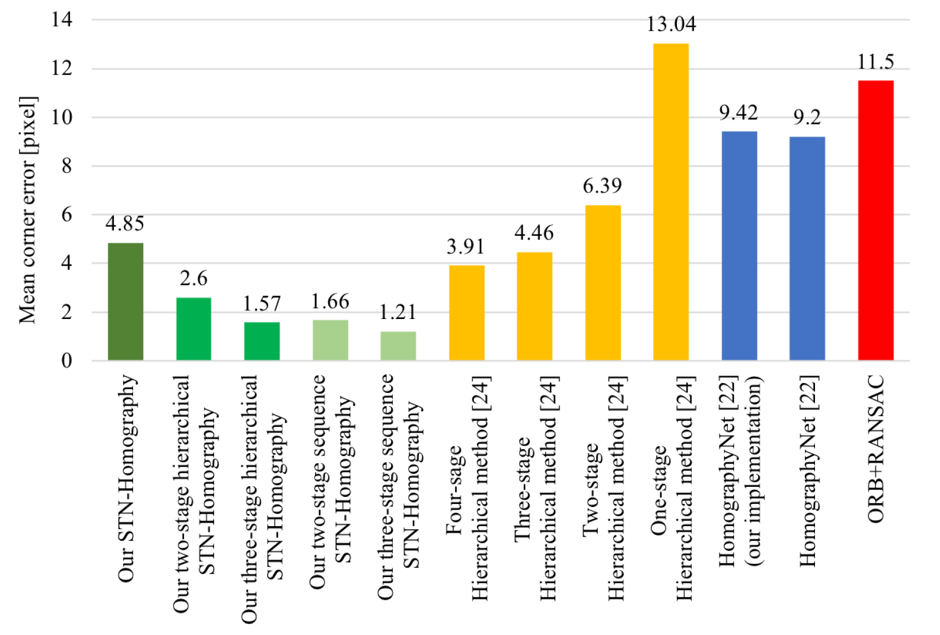
We experimentally compared the mean corner error of our STN-Homography model with other reported approaches. The approaches used for comparison consisted of one traditional and two convolutional methods. The selected traditional approach was based on the ORB+RANSAC method and the reference deep convolutional approaches are the HomographyNet by [22] and the hierarchical method by [24]. As shown in Figure 3, our single STN-Homography model can achieve a mean corner error of 4.85 pixels, which is much smaller than the mean error of the ORB+RANSAC method which is equal to 11.5 pixels, the mean error of the HomographyNet [22] of 9.2 pixels, and the error of the single-stage hierarchical method [24] which is equal to 13.04 pixels.

4. Hierarchical STN-Homography

4.1. Architecture of Hierarchical STN-Homography

Similar to the study of Nowruzi et al. [24], we also used a hierarchical model to successively reduce the estimation error of the homography matrix, as depicted in Figure 4. In each module, we used a new STN-Homography model to estimate the H ¯ b a _ i between patch_a_i (cropped from image_a_warp_i) and patch_b (cropped from image_b). Accordingly, the estimated H ¯ b a _ i will be used with the OpenCV library to warp image_a_warp_i to prepare image_a_warp_i+1 and patch_a_i+1 for the next module. To calculate the final result of the homography matrix between image_a and image_b, all homography matrix estimations of successive modules are multiplied together.
H ¯ b a = i = n , n 1 , ... , 1 H ¯ b a _ i
Warping with the predicted homography matrix from each module resulted in a visually more similar patch pair of patch_a_i and patch_b (or image pair of image_a_warp_i and image_b). This can be visualized as a geometric morphing process that takes one image and successively makes it to look alike the other, as shown in Figure 4.

4.2. Training, Results and Comparison with Other Approaches

As shown in Figure 4, when the hierarchical modules are trained, the training data of the current stage model depends on the predictions of the previous stage model, i.e., for each quadruplet training sample (patch_a_i, patch_b, H ¯ b a _ i , patch_a_t_i) of the stage i model, the patch_a_i, H ¯ b a _ i and patch_a_t_i all depend on the prediction results of the previous stage i-1 model. Therefore, we adopted a step-by-step training strategy. Using the three-stage hierarchical STN-Homography model as an example, first, we trained the stage 1 model and then used the trained stage 1 model to prepare the training dataset for the stage 2 model. Secondly, we trained the stage 2 model and then used the trained stage 1 and stage 2 models to prepare the training datasets for the stage 3 model. Finally, we trained the last stage 3 model. For the training of all stage models, we used the same training parameters as those used previously for the training of the STN-Homography model and we used the same loss weight of 1.0 for all losses of the model for simplicity. The only difference is that we used a total training steps of 130,000 for the stage 1 model and 90,000 steps for the stage i model (i = 2, 3).
As shown in Figure 3, the mean corner error of our three-stage hierarchical STN-Homography model is only 1.57 pixels. Compared with the outcomes of the study of DeTone et al. [22] which reported an error of 9.2 pixels, we decreased the mean corner error by 82.9%. Compared with the four-stage hierarchical model of [24], which has the mean corner error of 3.91 pixels, we also decreased the corner error by 59.8%.

4.3. Time Consumption and Predicted Results

We used TensorFlow [29] to implement our proposed hierarchical STN-homography model. During the test time, we achieved an average processing time of 4.87 ms for a single STN-Homography model on a GPU. When the same STN-Homography model is used at each stage of the hierarchical method, the overall computational complexity can be expressed by
d e = ( l m + l w ) × n
where d e is the end-to-end delay of the entire hierarchical model, l m is the average latency for each STN-Homography model, l w is the overhead of warping used to generate a new image pair, and n is the number of the stages used in the framework.
Table 2 shows the time consumption of our hierarchical STN-Homography model on a GPU. It can be observed that our three-stage hierarchical STN-Homography model results in an average processing time of 17.85 ms on a GPU. The real-time processing speed satisfies the requirements of most potential applications.
Figure 5 shows the predicted results of our three-stage hierarchical STN-homography model in some test samples. The green boxes in image_a and image_b represent the corresponding points for the ground truth, and the red boxes in image_a are transformed from the green boxes in image_b with the predicted homography matrix of image_a and image_b. As it can be observed from the figure, our model will achieve very small mean corner errors in stage 3.

5. Sequence STN-Homography

Although the proposed hierarchical STN-homography model yields a very small mean corner error, the training of a multistage hierarchical STN-Homography model is not an end-to-end training and relies on image_a when the training or testing is conducted (image_a was warped using the prediction result of the current stage to generate image_a_warp and patch_a for next stage). In this section, we proposed sequence STN-homography model that (a) can be trained in an end-to-end manner and (b) does not rely on image_a when the training or testing is conducted, i.e., sequential STN-homography takes the input image pair of patch_a and patch_b, and directly outputs the final predicted results of the homography matrix values between patch_a and patch_b (the homography matrix between image_a and image_b is the same as the homography matrix between patch_a and patch_b).

5.1. Architecture of Sequence STN-Homography

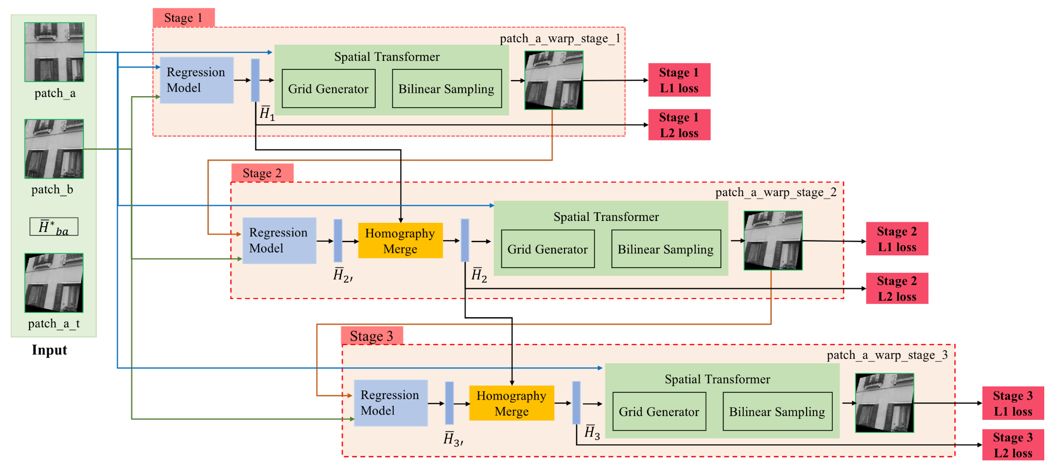
The sequence STN-homography is cascaded with several STN-Homography models, as depicted in Figure 6. The training input of the sequence STN-Homography model consists of quadruplet data of patch_a, patch_b, H ¯ b a * , and patch_a_t. Taking the there-stage sequence STN-homography as an example, in stage 1, the STN-Homography model takes the input image pair of (patch_a, patch_b) and outputs H ¯ 1 and patch_a_warp_stage_1, whereby H ¯ 1 is used to compute the L2 loss in combination with the ground truth H ¯ b a * , and patch_a_warp_stage_1 is used to compute the L1 loss with ground truth patch_a_t. In stage 2, the STN-Homography model takes the input image pair of (patch_a_warp_stage_1, patch_b) and outputs H ¯ 2 and patch_a_warp_stage_2, whereby H ¯ 2 is used to compute the L2 loss in combination with the ground truth H ¯ b a * , and patch_a_warp_stage_2 is used to compute the L1 loss with ground truth patch_a_t. In stage 3, the STN-Homography model takes the input image pair of (patch_a_warp_stage_2, patch_b) and outputs H ¯ 3 and patch_a_warp_stage_3, where H ¯ 3 is used to compute the L2 loss with the ground truth H ¯ b a * , and patch_a_warp_stage_3 is used to compute the L1 loss with the ground truth patch_a_t.
As show in Figure 6, in stage 2, H ¯ 2 = H ¯ 2 H ¯ 1 , where H ¯ 2 is the regression output representing the predicted normalized homography matrix between patch_a_warp_stage_1 and patch_b. In stage 3, H ¯ 3 = H ¯ 3 H ¯ 2 , where H ¯ 3 is the regression output representing the predicted normalized homography matrix between patch_a_warp_stage_2 and patch_b. We developed a tensor homography merge layer to compute H ¯ 2 , H ¯ 3 which is differentiable and can be trained with standard backpropagation, as shown in Figure 6.

5.2. Training, Results and Comparison with Other Approaches

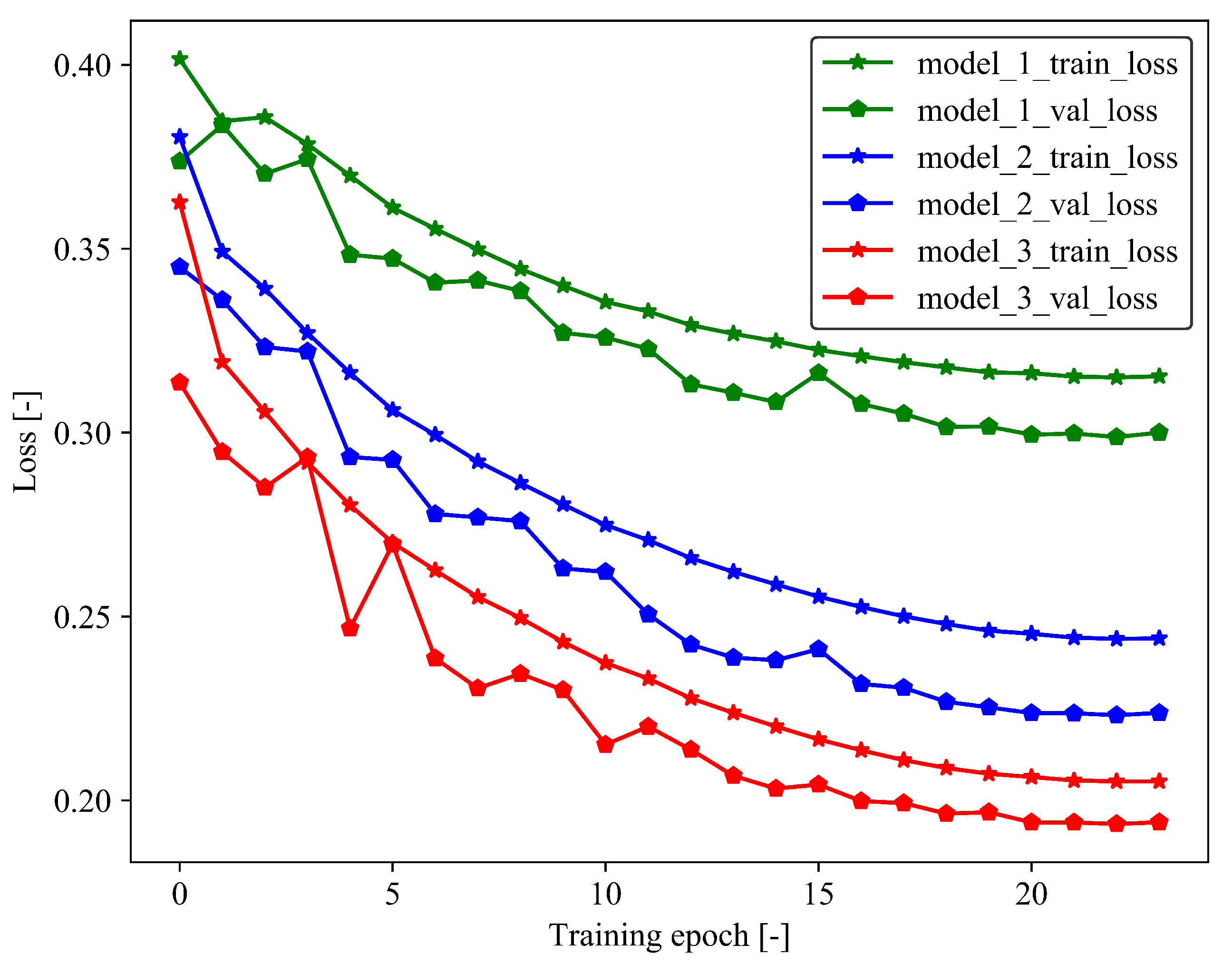
For simplicity, when training the sequence STN-Homography model, we used similar training parameters as those used for training single STN-Homography model and the loss weights of all losses of the sequence STN-Homography model are set to 1.0. The only difference is that when the two-stage sequence STN-Homography model was trained, we used 150,000 training steps, and when the three-stage sequence STN-Homography model was trained, we use 130,000 training steps and a smaller initial learning rate of 0.01 instead of 0.05. Figure 7 shows the training loss and validation loss during the training of three-stage sequence STN-Homography model.
Figure 3 shows the comparison of the mean corner error of our sequence STN-Homography model with other reported approaches. The two-stage sequence STN-Homography model achieves a mean corner error of 1.66 pixels, which is smaller than the previously proposed two-stage hierarchical STN-Homography model of 2.6 pixels and all other reported CNN-based methods [22,24]. The three-stage sequence STN-Homography model achieves a mean corner error of 1.21 pixels, which is smaller than the three-stage hierarchical STN-Homography model of 1.57 pixels. We found that the performance of the sequence STN-Homography model was better than that of the hierarchical STN-Homography model. The main reason is attributed to the fact that the sequence STN-Homography model can be trained in an end-to-end manner.

5.3. Time Consumption and Predicted Results

We also used TensorFlow to implement our proposed Sequence STN-Homography model. As shown in Table 3, during the test time, we achieved an average processing time of 9.55 ms for a two-stage sequence STN-homography model on a GPU and 13.85 ms for a three-stage sequence STN-Homography model on a GPU. Compared with Table 2, it is observed that the sequence STN-Homography model is faster than the hierarchical STN-Homography model.
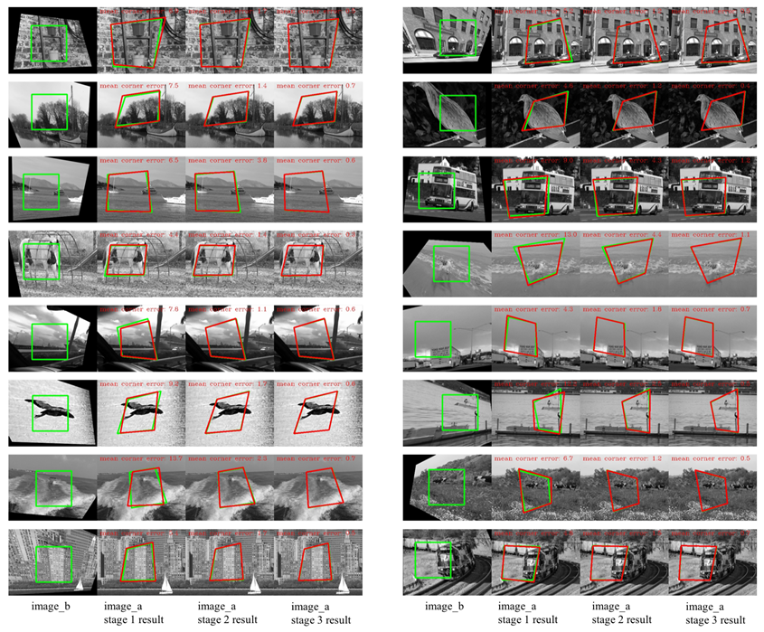
Figure 8 shows the predicted results of our three-stage sequence STN-Homography model in some test samples.

6. Conclusions

In this study, we showed that after pixel coordinate normalization of the homography matrix, we can apply a direct regression of the normalized homography matrix values with the proposed STN-homography model rather than estimate the alternative four-point homography. The mean corner error of the single STN-Homography model was 4.85 pixels, which was smaller than the state-of-the-art, one-stage, CNN-based four-point homography estimation methods. We also showed that with the hierarchical method, we could decrease the homography estimation error. Accordingly, the mean corner error of our three-stage hierarchical STN-Homography model was 1.57 pixels, which was superior to the state-of-the-art homography estimation outcomes. We also proposed a sequence STN-Homography model which could be trained in an end-to-end manner, and obtained superior results than the hierarchical STN-Homography model. The mean corner error of three-stage sequence STN-Homography model was only 1.21 pixels. The average processing times of our proposed three-stage hierarchical STN-homography model and three-stage sequence STN-Homography model on a GPU were 17.85 ms and 13.85 ms respectively, and they both satisfied the real-time processing requirements imposed in most potential applications.

Author Contributions

Conceptualization, Q.Z. and X.L.; methodology, Q.Z.; software, Q.Z.; validation, Q.Z.; formal analysis, Q.Z.; investigation, Q.Z.; resources, X.L.; data curation, Q.Z.; writing—original draft preparation, Q.Z.; writing—review and editing, X.L.

Funding

The authors disclosed receipt of the following financial support for the research, authorship, and/or publication of this article: This work was supported by the National Natural Science Foundation of China (No. U1613203, 51975514), Shenzhen Science and Technology Plan (No. JCYJ20170816172938761), and the Fundamental Research Funds for the Central Universities (No. 51221004).

Conflicts of Interest

The authors declare no conflict of interest.

References

  1. Brown, M.; Lowe, D.G. Automatic Panoramic Image Stitching using Invariant Features. Int. J. Comput. Vis. 2006, 74, 59–73. [Google Scholar] [CrossRef]
  2. Li, N.; Xu, Y.; Wang, C. Quasi-Homography Warps in Image Stitching. IEEE Trans. Multimed. 2018, 20, 1365–1375. [Google Scholar] [CrossRef]
  3. Chen, J.; Xu, Q.; Luo, L.; Wang, Y.; Wang, S. A Robust Method for Automatic Panoramic UAV Image Mosaic. Sensors 2019, 19, 1898. [Google Scholar] [CrossRef] [PubMed]
  4. Mur-Artal, R.; Montiel, J.M.M.; Tardos, J.D. ORB-SLAM: A Versatile and Accurate Monocular SLAM System. IEEE Trans. Robot. 2015, 31, 1147–1163. [Google Scholar] [CrossRef]
  5. Mur-Artal, R.; Tardos, J.D. ORB-SLAM2: An Open-Source SLAM System for Monocular, Stereo, and RGB-D Cameras. IEEE Trans. Robot. 2017, 33, 1255–1262. [Google Scholar] [CrossRef]
  6. Perdices, E.; Cañas, J. SDVL: Efficient and Accurate Semi-Direct Visual Localization. Sensors 2019, 19, 302. [Google Scholar] [CrossRef] [PubMed]
  7. Zhang, Z.; Hanson, A. 3D Reconstruction Based on Homography Mapping. In ARPA Image Understanding Workshop; Elsevier: San Francisco, CA, USA, 1996. [Google Scholar]
  8. Park, H.S.; Shiratori, T.; Matthews, I.; Sheikh, Y. 3D Reconstruction of a Moving Point from a Series of 2D Projections. In Computer Vision—ECCV 2010; Springer: Berlin/Heidelberg, Germany, 2010; pp. 158–171. [Google Scholar]
  9. Mei, C.; Benhimane, S.; Malis, E.; Rives, P. Efficient Homography-Based Tracking and 3-D Reconstruction for Single-Viewpoint Sensors. IEEE Trans. Robot. 2008, 24, 1352–1364. [Google Scholar] [CrossRef]
  10. Yang, J.; Li, H. Dense, accurate optical flow estimation with piecewise parametric model. In Proceedings of the 2015 IEEE Conference on Computer Vision and Pattern Recognition (CVPR), Boston, MA, USA, 7–12 June 2015. [Google Scholar]
  11. Xu, J.; Ranftl, R.; Koltun, V. Accurate Optical Flow via Direct Cost Volume Processing. In Proceedings of the 2017 IEEE Conference on Computer Vision and Pattern Recognition (CVPR), Honolulu, HI, USA, 21–26 July 2017. [Google Scholar]
  12. Lowe, D.G. Distinctive Image Features from Scale-Invariant Keypoints. Int. J. Comput. Vis. 2004, 60, 91–110. [Google Scholar] [CrossRef]
  13. Rublee, E.; Rabaud, V.; Konolige, K.; Bradski, G. ORB: An efficient alternative to SIFT or SURF. In Proceedings of the 2011 International Conference on Computer Vision, Barcelona, Spain, 6–13 November 2011. [Google Scholar]
  14. Fischler, M.A.; Bolles, R.C. Random sample consensus: A paradigm for model fitting with applications to image analysis and automated cartography. Commun. ACM 1981, 24, 381–395. [Google Scholar] [CrossRef]
  15. Badrinarayanan, V.; Kendall, A.; Cipolla, R. SegNet: A Deep Convolutional Encoder-Decoder Architecture for Image Segmentation. IEEE Trans. Pattern Anal. Mach. Intell. 2017, 39, 2481–2495. [Google Scholar] [CrossRef] [PubMed]
  16. He, K.; Gkioxari, G.; Dollár, P.; Girshick, R. Mask R-CNN. In Proceedings of the IEEE International Conference on Computer Vision, Venice, Italy, 22–29 October 2017; pp. 2961–2969. [Google Scholar]
  17. Cao, Z.; Hidalgo, G.; Simon, T.; Wei, S.E.; Sheikh, Y. OpenPose: Realtime Multi-Person 2D Pose Estimation using Part Affinity Fields. In Proceedings of the IEEE Conference on Computer Vision and Pattern Recognition, Honolulu, HI, USA, 21–26 July 2017; pp. 7291–7299. [Google Scholar]
  18. Mikolov, T.; Chen, K.; Corrado, G.; Dean, J. Efficient Estimation of Word Representations in Vector Space. arXiv 2013, arXiv:1301.3781. [Google Scholar]
  19. Shao, J.; Qu, C.; Li, J.; Peng, S. A Lightweight Convolutional Neural Network Based on Visual Attention for SAR Image Target Classification. Sensors 2018, 18, 3039. [Google Scholar] [CrossRef] [PubMed]
  20. Fischer, P.; Dosovitskiy, A.; Ilg, E.; Häusser, P.; Hazırbaş, C.; Golkov, V.; van der Smagt, P.; Cremers, D.; Brox, T. FlowNet: Learning Optical Flow with Convolutional Networks. In Proceedings of the IEEE International Conference on Computer Vision, Santiago, Chile, 7–13 December 2015; pp. 2758–2766. [Google Scholar]
  21. Ilg, E.; Mayer, N.; Saikia, T.; Keuper, M.; Dosovitskiy, A.; Brox, T. FlowNet 20: Evolution of Optical Flow Estimation with Deep Networks. In Proceedings of the IEEE Conference on Computer Vision and Pattern Recognition, Honolulu, HI, USA, 21–26 July 2017; pp. 2462–2470. [Google Scholar]
  22. DeTone, D.; Malisiewicz, T.; Rabinovich, A. Deep Image Homography Estimation. arXiv 2016, arXiv:1606.03798. [Google Scholar]
  23. Simonyan, K.; Zisserman, A. Very Deep Convolutional Networks for Large-Scale Image Recognition. arXiv 2014, arXiv:1409.1556. [Google Scholar]
  24. Nowruzi, F.E.; Laganiere, R.; Japkowicz, N. Homography Estimation from Image Pairs with Hierarchical Convolutional Networks. In Proceedings of the 2017 IEEE International Conference on Computer Vision Workshops (ICCVW), Venice, Italy, 22–29 October 2017. [Google Scholar]
  25. Nguyen, T.; Chen, S.W.; Shivakumar, S.S.; Taylor, C.J.; Kumar, V. Unsupervised Deep Homography: A Fast and Robust Homography Estimation Model. IEEE Robot. Autom. Lett. 2018, 3, 2346–2353. [Google Scholar] [CrossRef] [Green Version]
  26. Jaderberg, M.; Simonyan, K.; Zisserman, A.; Kavukcuoglu, K. Spatial Transformer Networks. In Proceedings of the Advances in Neural Information Processing Systems, Montreal, QC, Canada, 7–12 December 2015; pp. 2017–2025. [Google Scholar]
  27. Lin, T.Y.; Maire, M.; Belongie, S.; Hays, J.; Perona, P.; Ramanan, D.; Dollár, P.; Zitnick, C.L. Microsoft COCO: Common Objects in Context. In European Conference on Computer Vision; Springer: Cham, Switzerland, 2014; pp. 740–755. [Google Scholar]
  28. Loshchilov, I.; Hutter, F. SGDR: Stochastic Gradient Descent with Warm Restarts. arXiv 2016, arXiv:1608.03983. [Google Scholar]
  29. Abadi, M.; Agarwal, A.; Barham, P.; Brevdo, E.; Chen, Z.; Citro, C.; Corrado, G.S.; Davis, A.; Dean, J.; Devin, M.; et al. TensorFlow: Large-Scale Machine Learning on Heterogeneous Distributed Systems. arXiv 2016, arXiv:1603.04467. [Google Scholar]
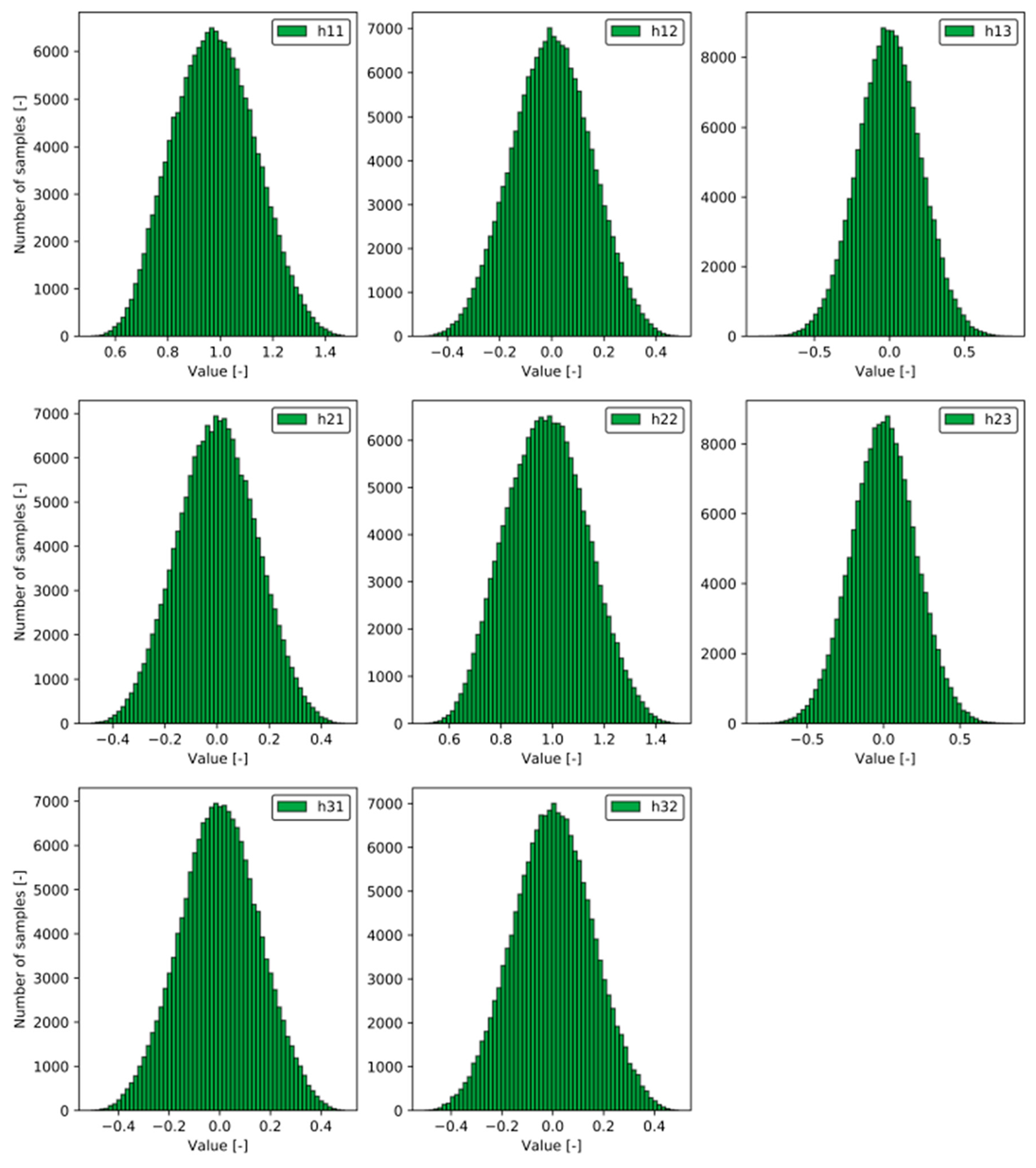
Figure 1. Histograms of H ¯ b a of the training dataset.
Applsci 09 05187 g001
Figure 2. Architecture of STN-Homography.
Applsci 09 05187 g002
Figure 3. Comparison of mean corner errors of various homography estimation approaches.
Applsci 09 05187 g003
Figure 4. Hierarchical STN-Homography architecture.
Applsci 09 05187 g004
Figure 5. Prediction results of our three-stage hierarchical STN-Homography model. We use the predicted homography matrix to transform the green box in image_b to the red box in image_a, while the green box in image_a represents the ground truth.
Applsci 09 05187 g005
Figure 6. Architecture of the three-stage sequence STN-homography model.
Applsci 09 05187 g006
Figure 7. Training curves showing the learning process of three-stage sequence STN-Homography model.
Applsci 09 05187 g007
Figure 8. Prediction results of our three-stage sequence STN-Homography model.
Applsci 09 05187 g008
Table 1. Impact of loss weights on the performance of the STN-Homography model.
Model NameL2 Loss WeightL1 Loss WeightMean Corner Error [Pixel]
STN-Homography1.01.05.83
STN-Homography1.010.021.86
STN-Homography1.00.16.21
STN-Homography10.01.04.85
STN-Homography0.11.06.24
Table 2. Time consumption of our hierarchical STN-homography model.
Model NameTime Consumption on a GPU [ms]
One-stage hierarchical STN-Homography4.87
Two-stage hierarchical STN-Homography11.46
Three-stage hierarchical STN-Homography17.85
Table 3. Time consumption of our Sequence STN-Homography model.
Model NameTime Consumption on a GPU [ms]
Two-stage Sequence STN-Homography9.55
Three-stage Sequence STN-Homography13.85