A High Efficiency Multistage Coder for Lossless Audio Compression using OLS+ and CDCCR Method

Abstract

In this paper, the improvement of the cascaded prediction method was presented. Three types of main predictor block with different levels of complexity were compared, including two complex prediction methods with backward adaptation, i.e., extension Active Level Classification Model (ALCM+) and extended Ordinary Least Square (OLS+). Our own approach to implementation of the effective context-dependent constant component removal block is also presented. Additionally, the improved adaptive arithmetic coder with short, medium and long-term adaptation was presented, and the experiment was carried out comparing the results with other known lossless audio coders against which our method obtained the best efficiency.

1. Introduction

The compression of audio and video signals is getting increasing attention as the transmission bandwidth is getting wider, storage media is getting cheaper and the requirement for better quality is growing. This has been proven by the dynamic work of the MPEG Group, operating from 1988 to today, and its impressive portfolio [1]. Among the developed standards and technologies, the lossless compression algorithms deserve special attention, which enables the conversion of the raw data into a compressed form and reconversion without losing any information.

Important purposes of lossless audio compression include recording storage, saving of records with high-quality sound on commercial media (e.g., DVDs, Blu-Ray, and CD (44100 sample/16 bit)) and selling songs in an online music stores for more demanding customers who are not satisfied with the quality of mp3 format [2]. Moreover, lossless mode is often required at the stage of music processing in a studio, advertising materials and in the production of radio and television programs, films, (post-production [3]) etc. In such cases, no lossy coding is used, which, at each iteration of sound editing, may cumulate additional distortions.

The motivation for our work is to improve the seemingly complete solution, in which we see areas of further development opportunities. We hope that through this research in the future the archiving and transmission of audio data in lossless form will become even better and more popular. Our solution is designed for target to use in static long-term archiving, such as the music database, source distribution of high-quality audio samples, where it is not required too often encoding but only distribution of coded files and encoding on client side. However, our solution does not give up and is also suitable for online encoding and decoding. Our solution is time symmetric, and is explained in more detail in Section 8.

Some popular examples of lossless audio compression codecs are APE (Monkey’s Audio) [4], Free Lossless Audio Coding (FLAC) [5], Shorten [6], WavPack [7], Nanozip [8], True Audio (TTA) [9], Tom’s verlustfreier Audiokompressor (TAK) [10], Lossless Audio (LA) [11] and the most often scientifically published one among lossless coders—MP4-ALS-RM23—which was published as a standard ISO/IEC 14496-3:2009 with the last revision in 2015 [12]. MP4-ALS-RM23 has many switches to customise the operation of the algorithm. Therefore, in the further part of the work, we distinguish two modes: default mode and the best mode, where default mode is used without any parameters, whereas the best mode uses switches in such a way as to obtain the best results for the tested base.

Lossless audio coders usually have two characteristic stages: modelling and fast compression, where the linear prediction is usually used for modelling, and entropy coders for fast compression [13]. Usually the modelling consists in replacing the current sample x(n) with its difference from the expected value $\widehat{x}(n)$ rounded to the nearest integer number:

$$e(n)=x(n)-\lfloor \widehat{x}(n)+0.5\rfloor .$$

(1)

The error signal e(n) has a distribution similar to the Laplace distribution, but because of the use of integers, in practice, the geometric distribution is used (see the Golomb code in Section 7).

The simplest constant prediction model is DPCM using the previous sample $\widehat{x}(n)=x(n-1)$. The basic predictive models are those with r-fixed coefficients (linear prediction in more detail is described in Section 2, see Formula (2)). A fixed predictor with a fixed set of r prediction coefficients can be used to efficiently encode various categories of audio data. The basic assumption of its universality is the fact that the sum of the coefficients should be 1 (this is a condition of the unbiased prediction estimator). The prediction order for the universal predictor (not associated with a specific audio signal) should not be too large (r ≤ 4).

The low order rule does not apply to, e.g., static predictors, in which the coefficients are determined for individual signal frames [14] (or entire sound files [15]), e.g., by means of minimising the mean square error (MMSE).

The publication of the results of our research has been divided into three stages of research. In [16], the general concept of new predictive cascade coding was presented, and in [17], the advantages of adaptive Golomb coding [18] are described. A description of the last widest stage of research work is in this article. Among the published solutions of this type, the highest efficiency is characterised by a cascaded RLS-LMS coder (see Section 5) [2] (implementation of MP4-ALS-RM23 in the best mode). Our method is a significant improvement in this cascading concept. Our coder has higher compression efficiency with a noticeable shortening of the total encoding time relative to work [16]; the experiments shown in Section 9 prove this. In Section 2 the basic prediction methods was described. In Section 3 and Section 4, we focus on simple and complex prediction methods with backward adaptation. In Section 4.2, the most effective OLS+ prediction block was described. Cascade connection of prediction block was described in Section 5. Details about removing context-dependent cumulate prediction error are presented in Section 6. In Section 7, a high efficiency version of the binary arithmetic coder using the Golomb code family was presented and analysis of practical aspects of prediction error encoder implementation is presented in Section 7.5. Schematic diagram of the proposed cascading audio data encoder method was presented in Section 8. The conclusion and summary are found in Section 10.

2. Basic Prediction Method

Among the basic prediction methods, i.e., constant and static linear predictive models, presented in the literature [19], lossless audio compression uses two approaches of an adaptive predictive modelling: forward adaptation and backward adaptation.

In the coding of audio, the method of determining the predicted value based on a linear prediction (which is based on the MMSE criterion) is most frequently used at the pre-modelling stage [13]. It requires a solution system of equations with r variables w_j that create vector of coefficients w = [w₁, w₂, … w_r]^T. Due to how the varied nature of the data in different parts of the sound work, methods with the current adaptation of the prediction coefficients allow achieving a high degree of compression.

Forward adaptation is an asymmetrical method of time, and its advantage is fast decoding time. The encoding process can be much longer because is possible perform initial coding multiple times, choosing the best parameters for the final version of the encoded file. In addition to the classic solutions used in MP4-ALS-RM23 (default version), it is possible look for better prediction models using extended data analysis [20], using other predictive techniques than the basic LPC computed using the Levinson–Durbin method, such as using Laguerre filters [21], and also due to cascading block connections with different lengths and prediction orders [22].

The predominantly used version is prediction with forward adaptation, which requires saving of prediction coefficients for individual encoded frames (the vector w of prediction coefficients is determined by optimising the mean error of prediction in the entire frame which requires access to it for analysis before coding [20,23]). In backward adaptation, the access to future samples is not required because the adaptation of vector of prediction coefficients is based on already coded samples [23,24]. The literature shows that prediction methods with backward adaptation achieve higher compression efficiencies because of the possibility of using higher orders of prediction and quick adaptation to changes in signal characteristics over time (adaptation of parameters every single sample of data). For this reason, this work focuses on this approach. In addition, we are currently focusing only on the CD standard parameters, i.e., 44,100 samples per second, with a resolution of 16 bits, as it is still the most common format for commercial use of music.

In stereo CD standard existing dependencies between channels allow to use in r-order predictive models using samples from both channels, left x_L(n − i) and right x_R(n − j).

$$\begin{array}{l}{\widehat{x}}_L\left(n\right)={\displaystyle \sum _{i=1}^{r_L}{a}_i\cdot x_L\left(n-i\right)+{\displaystyle \sum _{j=1}^{r_R}{b}_j\cdot x_R\left(n-j\right)}}\\ {\widehat{x}}_R\left(n\right)={\displaystyle \sum _{j=1}^{r_L}{c}_j\cdot x_R\left(n-j\right)+{\displaystyle \sum _{i=0}^{r_R-1}{d}_i\cdot x_L\left(n-i\right)}}\end{array}$$

(2)

Based on the general form w_Ch = [w₁, w₂, … w_r]^T, according to Formula (2) (where Ch is the channel L (left) or R (right)), we can distinguish vectors of prediction coefficients for the left channel $w_L={\left[a_1,a_2,\dots ,a_{r_L},b_1,b_2,\dots ,b_{r_R}\right]}^{\mathrm{T}}$ and for right channel $w_R={\left[c_1,c_2,\dots ,c_{r_L},d_0,d_1,\dots ,d_{r_R-1}\right]}^{\mathrm{T}}$. There are two formulas because by coding (decoding) the value of the right channel sample x_R(n), there is already access to the current sample of the left channel x_L(n). The result of the bit average can be influenced by the selection of which channels are coded in the first order. Note that the r_L ordering in both cases concerns the set of samples of the currently coded channel, whereas r_R is number samples of the opposite channel, in addition r = r_L + r_R.

There is a problem with the selection of the universal r_R/r_L ratio. The most common proportions in the literature are 1:1 and 1:2, after completing the bit-minimising experiments (in forward adaptation mode) it turned out that depending on the size of frame (2^q), the best order of prediction r is changing (within the test database). Also, the increase order of the prediction r leads to a decreasing value of the ratio r_R/r_L [14]. For backward adaptation (methods described in Section 4), good results were obtained for a 1:1 proportion.

3. Simple Prediction Method with Backward Adaptation

The basic advantage of adaptation of prediction coefficients is the ability to adjust w_j coefficients to the variability of the signal over time. An additional characteristic, only for backward adaptation, is the lack of the need for initial analysis of the entire signal frame, which must be carried out using, for example, static models (forward adaptation), where in the case of MMSE, one or many systems of equations with r unknowns must be determined and solved.

One of the simplest methods of adapting prediction coefficients is Least Mean Square (LMS). In the basic version it is less effective compared to even the RLS, ALCM+, and OLS+ methods discussed in the next section, as it is relatively slow convergence to achieve the results obtained than MMSE with forward adaptation.

Adaptation of prediction coefficients in LMS is done according to the following relation,

$$w(n+1)=w(n)+\mu \cdot e(n)\cdot x(n)$$

(3)

where vector x(n) = [x(n − 1), x(n − 2), …, x(n − r)]^T contains r samples of the currently encoded channel. Most often, the vector w(0) is initialised as w(0) = [β, 0, …, 0] where β = 0 or β = 1. The complexity of this procedure is linear O(r), therefore it is suitable for building high order predictive models.

The step size, µ, is very important here, as it determines the speed of adaptation of the vector coefficients w(n) to the current signal characteristics. Proper selection of this value has a significant impact on the final bit average of the encoded audio track and it is difficult to find a universal experimental value, the same problem applies to the value of the prediction order.

To a large extent, these problems can be solved by introducing an extended version of this method. The standardised version of Normalised LMS (NLMS) [25] has a higher rate of adaptation due to the energy level of the last encoded signal samples. This involves changing the learning factor:

$$\mu (n)=\frac{\mu }{1+x^{\mathrm{T}}(n+1)\cdot x(n+1)}=\frac{\mu }{1+{\displaystyle \sum _{i=0}^{r-1}{x}^2(n-i)}}.$$

(4)

In our solution, we proposed to develop Formula (3) by introducing a scaling factor, which is located on the diagonal of the matrix C = diagonal ([0.995¹ 0.995² … 0.995^r]), to the formula for adaptation of prediction coefficients by ES-NLMS method (an idea taken from the exponentially weighted step-size (NLMS) [26]), and the value of 0.995 was selected experimentally:

$$w_{\mathrm{NLMS}}(n+1)=w_{\mathrm{NLMS}}(n)+\mu (n)\cdot e(n)\cdot C\cdot x(n).$$

(5)

4. Complex Prediction Method with Backward Adaptation

In [24], the authors presented a highly efficient cascade method combining several stages of prediction (DPCM + RLS + LMS1 + LMS2 + LMS3 − see Section 5) with backward adaptation (implementation the MP4-ALS-RM23 – in the best mode). It is a method using high complexity of the recursive least square (RLS) block and a large summary number of prediction coefficients undergoing adaptation in LMS1, LMS2 and LMS3 blocks.

In RLS, the backward adaptation method of linear prediction coefficients has the computational complexity O(r²), which is much greater compared to NLMS while offering faster and more effective prediction with a small order of prediction (details of adaptation of coefficients in RLS are described in [24]). To further improve its performance, it is proposed to use preliminary data modelling in the form of a DPCM block. This allows reducing the dynamics of the signal fed to the input of the RLS block (see Figure 1). In this figure, the RLS predictive block is the only one in the cascade approach that uses interchannel relationships in stereo. Similarly, the cases of ALCM+ and OLS+ are described in the next two items.

4.1. ALCM+

In the proposed solution, the complexity of the main prediction block can be significantly reduced by replacing the RLS block with the rapid ALCM+ method. In the ALCM+ method, the prediction coefficients adaptation procedure has a linear complexity relative to the order of prediction and does not require any square matrix to be adapted.

4.1.1. ALCM Rapid Adaptation Method

The adaptive prediction method Activity Level Classification Model (ALCM) [27] was developed in the 1990s for image coding purposes. It is characterised by a lower, though similar, computational complexity compared to the classic LMS solution. Originally, the method operated on linear prediction models of the fifth or sixth order, with the set of all coefficients in each step being adapted (by the constant μ = 1/256 at 8-bit samples) only two (up to six in the ALCM+ version proposed in this paper) properly selected.

Despite its simplicity, this method gives relatively good results also with regard to audio coding. The method is applied with respect to the interchannel stereo mode, and therefore two prediction orders {r_L, r_R} correspond to the data from the currently coded and opposite channels, and the total prediction order of the ALCM+ method equals r = r_L + r_R. Generalising some formulas, we can introduce the designation Ch (channel) in place of L (left) and R (right).

To increase the efficiency of the method, the initial DPCM block is used, the DPCM block returns an $e_{Ch}^{\mathrm{DPCM}}(n)$ error at the time n, which is buffered as a set of errors from previous i-th moments marked as g(i). Therefore the ALCM+ input stream consists of elements that are the difference of two consecutively coded samples g(i) = x(n − i) − x(n − i − 1). Assuming that the left channel sample are encoded before right channel sample, the ALCM+ encoder input vectors at time n have the following form; for the left channel, g_L(n) = [g_L(1), g_L(2), …, g_L(r)]^T = [x_L(n − 1) − x_L(n − 2), x_L(n − 2) − x_L(n − 3), …, x_L(n − r_L) − x_L(n − r_L− 1), x_R(n − 1) − x_R(n − 2), x_R(n − 2) − x_R(n − 3), …, x_R(n − r_R) − x_R(n − r_R− 1)]^T, while for the right channel g_R(n) = [g_R(1), g_R(2), …, g_R(r)]^T = [x_R(n − 1) − x_R(n − 2), x_R(n − 2) − x_R(n − 3), …, x_R(n − r_L) − x_R(n − r_L − 1), x_L(n) − x_L(n − 1), x_L(n − 1) − x_L(n − 2), …, x_L(n − r_R + 1) − x_L(n − r_R)]^T.

Due to the specificity of the vector g_Ch(n), the predicted values are determined as

$${\widehat{x}}_{Ch}(n)=x_{Ch}(n-1)+{\displaystyle \sum _{i=1}^r{w}_{Ch}(i)\cdot g_{Ch}(i)}.$$

(6)

4.1.2. The Principle of Adaptation in Our Proposition of the Improved Version of ALCM+

In the new version of ALCM+ presented in this paper, it was proposed to introduce five parallel predictive models with orders r_j of r = {10, 22, 30, 56, 110}, respectively, where the orders of predictions have been chose as a result of many experiments to optimise compression efficiency for the learning base.

The predicted value is determined as the arithmetic mean of these five prediction models:

$${\widehat{x}}_{Ch}(n)=x_{Ch}(n-1)+\frac{1}{5}\cdot {\displaystyle \sum _{j=1}^5{\displaystyle \sum _{i=1}^{r_j}{w}_{Ch}^{(j)}(i)\cdot g_{Ch}(i)}},$$

(7)

where Ch is the indicator of L (left) or R (right) channel and j is the number of one of the five prediction models.

In each of these models, after coding the next sample, six prediction coefficients are adapted. For this purpose, the three highest and lowest values of r_j from the g_Ch(i) elements from the vector g_Ch(n) are determined, where $i\in \overline{1;r_j}$.. Denoting these three elements, respectively, as the smallest value:

$$g_{Ch}(q_{Ch(1)}^{(j)})\le g_{Ch}(q_{Ch(2)}^{(j)})\le g_{Ch}(q_{Ch(3)}^{(j)})$$

(8)

and three largest values:

$$g_{Ch}(p_{Ch(3)}^{(j)})\le g_{Ch}(p_{Ch(2)}^{(j)})\le g_{Ch}(p_{Ch(1)}^{(j)}).$$

(9)

Then, for everyone j-th $(j\in \overline{1;5})$ predictive models (if assuming that the condition $g_{Ch}(q_{Ch(1)}^{(j)})<g_{Ch}(p_{Ch(1)}^{(j)})$ is true), the following adaptation prediction coefficients are used (see Algorithm 1).

Algorithm 1: Adaptation of prediction coefficients by predictive models.

$$\begin{gathered} \mathrm{if} {\widehat{x}}_{Ch}(n)<x_{Ch}(n)\mathrm{then} \{ \\ \hspace{1em}\hspace{1em}{w}_{p_{Ch(k)}^{(j)}}^{(j)}(n+1)=w_{p_{Ch(k)}^{(j)}}^{(j)}(n)+{\mu }_{Ch(k)}^{(j)},\mathrm{for} k=\{1, 2, 3\} \\ \hspace{1em}\hspace{1em}{w}_{q_{Ch(k)}^{(j)}}^{(j)}(n+1)=w_{q_{Ch(k)}^{(j)}}^{(j)}(n)-{\mu }_{Ch(k)}^{(j)}, \mathrm{for} k=\{1, 2, 3\} \\ \} \mathrm{else} \mathrm{if} {\widehat{x}}_{Ch}(n)>x_{Ch}(n)\{ \\ \hspace{1em}\hspace{1em}{w}_{p_{Ch(k)}^{(j)}}^{(j)}(n+1)=w_{p_{Ch(k)}^{(j)}}^{(j)}(n)-{\mu }_{Ch(k)}^{(j)},\mathrm{for} k=\{1, 2, 3\} \\ \hspace{1em}\hspace{1em}{w}_{q_{Ch(k)}^{(j)}}^{(j)}(n+1)=w_{q_{Ch(k)}^{(j)}}^{(j)}(n)+{\mu }_{Ch(k)}^{(j)},\mathrm{for} k=\{1, 2, 3\} \\ \} \end{gathered}$$

The modifying step-size ${\mu }_{Ch(k)}^{(j)}$ value is determined as follows,

$${\mu }_{Ch(k)}^{(j)}=\min \{2^{-6};{\overline{\mu }}_{Ch(k)}^{(j)}\},$$

(10)

where,

$${\overline{\mu }}_{Ch(k)}^{(j)}=\frac{\left|x_{Ch}(n)-{\widehat{x}}_{Ch}(n)\right|}{2^3\cdot {\displaystyle \sum _{k=1}^3{\alpha }_k\cdot \left(g_{Ch}(p_{Ch(k)}^{(j)})-g_{Ch}(q_{Ch(k)}^{(j)})\right)}}$$

(11)

and α_k = {1; 0.5; 0.5}.

4.2. OLS+

Extended version of Ordinary Least Square (OLS+) is characterised by a slightly more computational complexity than RLS. In addition to the update (O(r²) complexity, as in RLS) of the square matrix R(n) autocovariance (r×r dimensions), an additional procedure for determining the inverse matrix with the O(r³) complexity is required.

In the OLS+ method, prediction coefficients are calculated adaptively, individually for each coded sample, minimising the mean square error in a certain limited backward area. The influence of older samples is limited by the use of the forgetting effect determined by the factor f_f.

In OLS+, the basic matrix equation used to calculate the vector w(n) has been extended by the element u_bias, which comes from the principles of ridge regression [28]. The u_bias element modifies the main diagonal values in autocovariance matrix R(n). This prevents the occurrence of a singular matrix and also improves the overall efficiency of modelling. The vector of prediction coefficients is obtained by solving the matrix equation (for simplification the designations of L and R channels have been removed at this point, remembering that for each channel, there are separate R_Ch(n) matrix’s and vectors w_L(n) and w_R(n), as described in Section 2, Formula (2)):

$$\mathbf{w}(n+1)={\mathbf{R}}_{\mathrm{bias}}^{-1}(n+1)·\mathbf{q}(n+1),$$

(12)

where the matrix R_bias(n + 1) is complemented by a value u_bias(n + 1):

$$R_{\mathrm{bias}}(n+1)=R(n+1)+u_{\mathrm{bias}}(n+1)\cdot I,$$

(13)

where I is a identity matrix. In [16], u_bias was a fixed value. Based on the work in [28], it was proposed to determine the u_bias in the following way,

$$u_{\mathrm{bias}}(n+1)=\frac{r\cdot (1-f_f)\cdot c_{\mathrm{OLS}}\cdot e^2(n)}{\max \{1,w_j^2(n)\}}, \mathrm{for}j\in \overline{1;r}.$$

(14)

Elements R_j,i(n + 1) of the matrix R(n + 1) with dimensions r×r are updated after encoding each subsequent sample as follows.

R_j,i(n + 1) = c_OLS⋅x(n − i)⋅x(n − j) + f_f⋅R_j,i(n).

(15)

Therefore, the elements q_j(n + 1) of the vector q(n + 1) with dimensions r×1 are updated as follows.

q_j(n + 1) = c_OLS⋅x(n)⋅x(n − j)+ f_f⋅q_j(n).

(16)

For the first 100 samples, the predictive model is not determined, due to the insufficient representativeness of data in the autocovariance matrix, so a simple DPCM prediction model of the first order is used. The weight

$$c_{\mathrm{OLS}}={(s_{err}(n+1)+2)}^{-\frac{3}{4}}$$

(17)

is dependent on the calculated iterative value

s_err(n + 1) = h_f⋅s_err(n)+ |e(n)|.

(18)

The introduction of c_OLS is intended to reduce the role of input data for which larger absolute prediction errors |e(n)| are obtained. The best compression results were obtained at r = 20 (predictor using 10 samples back from both channels) and with forgetting factors f_f = 0.9983 and h_f = 0.69.

The OLS+ method has greater computational complexity than in case of RLS method because of need to inverse the matrix. An advantage of OLS+ is the better efficiency of the predictive model, obtained by using additional operations on autocovariance matrix before it is inverse, according to the Formulas (13), (17), and (18). It is different to the case of the method of fast adaptation in RLS as it applies to the already inverted matrix, which is more sensitive and difficult to determine the common forgetting factor that ensures proper efficiency in all the test base files. For this reason, in the MP4-ALS-M23 forgetting factor has a universal value equal 1.

5. Cascade Connection of Prediction Method

In the solution described in [24] based on prediction models with backward adaptation, a cascade connection of individual five stages (blocks) is used. The first one is the constant predictor DPCM, whereas the second block uses the RLS method for example with an order r_RLS = 16 (using w vector with eight w_j coefficients per channel in stereo mode [24,29]). The remaining three blocks (see Figure 1) use the NLMS method (see Section 3), wherein each subsequent block the smaller prediction order is used; the outputs of subsequent blocks are dependent on the values calculated in the preceding blocks. For the NLMS blocks, the following prediction orders were proposed, r_i = {384, 112, 16}.

Our previous approach in [16] also uses a cascade of five blocks including three subsequent blocks of the modified version of NLMS with orders {1000, 25, 10}. In the solution proposed here, which is an extension of the codec from work [16], the prediction order in the middle NLMS block has been increased from r = 25 to r = 380. Instead of the OLS block, an improved version of OLS+ has been introduced, whose simplified version has been successfully used earlier in lossless image compression [30,31].

In Section 4, two new approaches to the initial prediction stage (ALCM+ and OLS+) are proposed. In Figure 2, the proposed solution with the ALCM+ block (of lower complexity) is shown. The higher complexity version differs only in that the OLS+ block has been introduced in place of DPCM and ALCM+ blocks.

If we define w^(j)(n) as a vector that stores the prediction coefficients used in the j-th stage of the cascade, then the relationships between the successive stages of the cascading system are as follows,

y₁(n) = x(n − 1)

(19)

$$y_j(n)={\displaystyle \sum _{i=1}^{r_j}{w}_i^{(j)}(n)\cdot e_{j-1}(n-i)}, \mathrm{for}j>1$$

(20)

e₁(n) = x(n) − y₁(n),

(21)

e_j(n) = e_j−1(n) − y_j(n), for j > 1.

(22)

Compared to the original approach presented in [24,29], the initial DPCM block has been abandoned (y₁(n) = 0), and the RLS block has been replaced with the extended OLS+ block, where interchannel dependencies are removed.

After K stages of prediction blocks as the last block of determining the final version of the predicted $\widehat{x}(n)=y_K$ value, the method of removing the cumulative prediction error was added where the C_mix value is calculated as the constant component (bias), depending on the individual number of the context for each successively coded x(n) sample (see Section 6). This method earlier was successfully used only in lossless image compression [32]. This block is marked as Context-Dependent Constant Component Removing (CDCCR) and, similarly to the development of NLMS blocks, has been described in detail in Section 3.

The final prediction error is calculated from

$$e(n)=x(n)-\lfloor y_1(n)+y_2(n)+\dots +y_K(n)+C_{\mathrm{mix}}+0.5\rfloor .$$

(23)

The last two blocks (marked in Figure 2 as Golomb Code and CABAC) in the cascade audio data compression system proposed here are used to efficiently code prediction errors e(n) into the resulting binary data stream (see Section 7).

In

Table 1. Comparison first-order entropy using DPCM + ALCM+, DPCM + RLS and OLS+ without and with connection three Normalised Least Mean Square (NLMS) blocks in cascade.

	Without Three NLMS Blocks			With Three NLMS Blocks in Cascade
File	ALCM+	RLS	OLS+	ALCM+	RLS	OLS+
ATrain	8.3507	8.1934	8.2817	7.7531	7.7088	7.6675
BeautySlept	9.8388	9.7497	9.8416	8.8806	8.8194	8.7118
chanchan	10.3974	10.3807	10.3537	10.2931	10.2278	10.1932
death2	6.4038	7.0594	6.5856	6.6436	6.9072	6.3777
experiencia	11.5514	11.5710	11.5828	11.3683	11.3198	11.2973
female_spech	5.8583	5.6922	5.7743	5.7413	5.5754	5.5857
FloorEssence	10.4917	10.4153	10.3952	10.1471	10.0712	10.0134
ItCouldBeSweet	9.6181	9.3986	9.4630	9.3595	9.2149	9.2689
Layla	10.6077	10.5589	10.6175	10.2457	10.1759	10.1559
LifeShatters	11.1976	11.1492	11.1698	11.0151	10.9659	10.9481
macabre	10.1090	10.1758	10.1952	9.5819	9.5489	9.5070
MaleSpeech	5.8177	5.7310	5.7632	5.7054	5.6156	5.5813
SinceAlways	11.5095	11.3424	11.3904	11.3111	11.2132	11.2034
thear1	12.0500	11.9855	12.0026	11.9159	11.8660	11.8490
TomsDiner	8.2075	7.9984	8.0337	7.9481	7.7740	7.7600
velvet	11.4401	11.2113	11.1379	11.0710	10.8298	10.7851
Average 1st order entropy	9.5906	9.5383	9.5368	9.3113	9.2396	9.1816

, the first-order entropy results for 16 test files are presented (more about first-order entropy in Section 7). The first three columns contain entropy results after applying DPCM + ALCM+, DPCM + RLS and OLS+, respectively. The last three columns present the results of the same set, but with an additional three NLMS blocks with prediction orders {1000, 380, 10}, respectively. In both RLS and OLS+, blocks the prediction order of r = 20 was used (the average first order entropy of the whole database was bold in the last row of Table 1.).

An important conclusion is that the advantage of OLS+ over RLS is only noticeable after including three NLMS blocks in the cascade prediction system. This shows how unobvious the purely theoretical approaches can be. Only practical experiments (see [24]) allow determining the final universal form of the cascade prediction system.

The final solution proposed in this work is therefore the cascade shown in Figure 2 after taking into account the changing of the first two DPCM + ALCM+ blocks into the OLS+ block.

6. Removing Context-Dependent Cumulate Prediction Error

Often prediction methods can introduce constant (bias) components in predetermined prediction errors. The nature of component depends on the properties of a context defined as (heuristically selected) a set of features the nearest neighbourhood. In practice, the division into a large number of contexts is used (it can be from several hundred to several thousand), which precisely allows to determine the type of the closest neighbourhood of the coded sample using different features of the previous few samples and previously coded prediction errors. The context number can be represented, e.g., as the i-bit-number, where each bit can be determined in a separate way; for example, by two-state quantisation of the module of the previous prediction error, checking if the condition |e(n − 1)| > 50 or checking the condition x(n − 1) > x(n − 2).

For example, with i = 11 different rules of this type, 2048 contexts can be created, and each can adaptively calculate a separate average or median value from previous prediction errors that can be subtracted from the predicted prediction error at the next occurrence of the given context in the coding step.

This idea is commonly used in relation to image coding [32]. The adaptive method of removing a constant component is used both in the CALIC [33] and JPEG-LS algorithms [34].

The algorithms are shown in Algorithm 2, where j is the context number, $S_{(j)}^{(Ch)}$ is the current cumulative value of prediction error $e_K^{(Ch)}(n)$ in the given context, $N_{(j)}^{(Ch)}$ is the count of occurrences of the given context and $C_{(j)}^{(Ch)}$ is the current correction value that should be added to the predicted value e_K(n) as its corrective value.

Algorithm 2: Our authorial algorithm of adaptation $C_{(j)}^{(Ch)}$ value based on the CALIC method.

Initial value: $$\begin{gathered} \hspace{1em}\hspace{1em}{S}_{(j)}^{(Ch)}:= C_{(j)}^{(Ch)}:= 0, \mathrm{for} \mathrm{every} j; \\ \hspace{1em}\hspace{1em}{N}_{(j)}^{(Ch)}:= 4, \mathrm{for} \mathrm{every} j; \\ \hspace{1em} \\ \mathrm{if} | e_K^{(Ch)}(n)| < 4\cdot \sqrt[4]{Var(X)} \mathrm{then} \{ \\ \hspace{1em}\hspace{1em}{S}_{(j)}^{(Ch)}:= S_{(j)}^{(Ch)}+ e_K^{(Ch)}(n); \\ \hspace{1em}\hspace{1em}{N}_{(j)}^{(Ch)}:= N_{(j)}^{(Ch)}+ 1; \\ \} \\ {C}_{(j)}^{(Ch)}:= S_{(j)}^{(Ch)}/N_{(j)}^{(Ch)}; \end{gathered}$$

The periodic forgetting technique is also useful, which additionally allows adjustment of the values of the constants $C_{(j)}^{(Ch)}$ to the local properties of the j-th context, if $N_{(j)}^{(Ch)}$ is greater than 127 then $N_{(j)}^{(Ch)}$ is set on 64 and $S_{(j)}^{(Ch)}$ is set as $S_{(j)}^{(Ch)}$/2.

To remove a context-dependent constant component, instead of the arithmetic mean used in CALIC, it is possible to use the median of a set of prediction errors previously appearing in a given context.

Also, in this case, it is worthwhile to additionally use the technique of forgetting periodic after the occurrence counter of $N_{(j)}^{(Ch)}$ j-th context has reached the value of 128. This improves the overall efficiency of compression while also reducing the size of the vector to 64 elements, which store the prediction errors that appear earlier in the given context. Forgetting periodic consists in reducing the vector by half of 128 elements by removing the first 32 and last 32 elements sorted ascending vector which stores the prediction errors that appear earlier in the given context.

In presented codec this solution was proposed to encode an audio signal with equally good effect as the last block CDCCR in the cascade as an improvement of the value of the predicted coded samples. Due to this work a bit average can be shortened by up to 1% (depending on the input data and the efficiency of previous prediction blocks).

The idea is based on the determination of 4 types of contexts, and each of them is used twice (using the arithmetic mean and medians marked with the AVE and MED symbols, respectively). In this way, eight constant components are created, and, on the basis of which, the final weighted $C_{\mathrm{mix}}^{(Ch)}$ is determined by

$$C_{\mathrm{mix}}^{(Ch)}=\frac{1}{36}\left(4\cdot {\displaystyle \sum _{i=1}^4{C}_{(j(i))}^{(Ch)\mathrm{AVE}}}+5\cdot {\displaystyle \sum _{i=1}^4{C}_{(j(i))}^{(Ch)\mathrm{MED}}}\right).$$

(24)

The high efficiency of the mixed method of constant component correction results from the principles of mixing correction values that are burdened by some of level of uncertainty, which may individually deteriorate in some situations the final level of prediction error (incorrect prediction of correction values). This is prevented by mixing (weighted average) that causes the correlation of these uncertain correction values to a large extent. At the same time, this method reduces the chances of occurrence of the asymmetry effect of the distribution, which can be manifested by the occurrence in the given j-th context of differences between the position in the histogram, indicated as the arithmetic mean $C_{(j)}^{(Ch)}$ of prediction errors, and the actual position indicating in the histogram the maximum probability (histogram of the Laplace distribution has one maximum), indicated in [35].

In

Table 2. A set of decision rules for determining number of contexts.

Bits	Condition
αi	2⋅x(n − i) − x(n − i − 1) $> \widehat{x}(n)$, for i = {1, 2, 3}
αi + 3	x(n − i $> \widehat{x}(n)$, for i = {1, 2, 3}
αi + 6	e(n − i) > 0, for i = {1, 2}
αi + 8	e(n − i) > e(n − i − 1), for i = {1, 2, 3}
αi + 11	$\left|x(n-i)-\widehat{x}(n)\right|>T_h(i)$, for i = {1, 2, 3, 4}, Th(i) = {250, 100, 1500, 1500}
αi + 15	$\left|e(n-i)\right|>T_h(i)$, for i = {1, 2}, Th(i) = {50, 150}
αi + 17	$\left|e(n-i)\right|>T_h(i)$, for i = {1, 2}, Th(i) = {750, 900}
αi + 19	x(n − i) > x(n − i − 1), for i = {1, 2}
α22	1.75⋅x(n − 1) − 0.75⋅x(n − 2) > $\widehat{x}(n)$

is a set of decision rules based on which the numbers of contexts are determined. Decisions are two-state (binary) quantizer that returns the value of bit 0 or 1 (individual bits are defined here as α_i), which corresponds to the fulfilment or non-fulfilment of a given condition (YES/NO answer). As they are partially repeated in subsequent ways of building the context number, they will be listed Table 2, and the construction rules for the four types of context number are described in the following Section 6.1, Section 6.2, Section 6.3 and Section 6.4.

6.1. First Type of Context

The number 1 of the context type is determined as a ten-bit number of κ₉κ₈κ₇κ₆κ₅κ₄κ₃κ₂κ₁κ₀ characters, where κ_{i − 1} = α_i for i = {1, 2, …, 8}. The last two bits of κ₉κ₈ are determined using a four-state quantizer of the sum of S₁ with three thresholds {50, 250, 700}, where

$$S_1={\displaystyle \sum _{i=1}^5\left|x(n-i)-\widehat{x}(n)\right|}.$$

(25)

6.2. Second Type of Context

The number 2 of the context type is determined as a eleven-bit number of κ₁₀κ₉κ₈κ₇κ₆κ₅κ₄κ₃κ₂κ₁κ₀ characters, where κ_{i − 1} = α_{i + 19} for i = {1, 2}, κ_{i + 1} = α_{i + 8} for i = {1, 2, 3}, κ_{i + 4} = α_{i + 11} for i = {1, 2, 3, 4} and κ_{i + 8} = α_{i + 15} for i = {1, 2}.

6.3. Third Type of Context

The number 3 of the context type is determined as a eleven-bit number of κ₁₀κ₉κ₈κ₇κ₆κ₅κ₄κ₃κ₂κ₁κ₀ characters, where κ_{i − 1} = α_{i + 19} for i = {1, 2}, κ_{i + 1} = α_{i + 8} for i = {1, 2}, κ_{i + 3} = α_{i + 3} for i = {1, 2}, κ_{i + 5} = α_{i + 17} for i = {1, 2} and κ₈ = α₂₂. The last two bits of κ₁₀κ₉ are determined using a four-state quantizer of the sum of S₂ with three thresholds {100, 400, 1550}, where

$$S_2={\displaystyle \sum _{i=1}^4\frac{1}{\sqrt{i}}\left|x(n-i)-\widehat{x}(n)\right|}.$$

(26)

6.4. Fourth Type of Context

The number 4 of the context type is determined as a number that is a composite of three values. The first two are determine as six-state quantizer with thresholds {-100, -10, 0, 10, 100} for value d₁ and d₂, respectively, where d_i = x(n − i) − x(n − i − 1), for i = {1, 2}. The third value of the context number is the six-bit κ₅κ₄κ₃κ₂κ₁κ₀ character value, where κ_{i − 1} = α_{i + 8} for i = {1, 2}, κ₂ = α₂, whereas three bits κ₅κ₄κ₃ are determined using an eight-state quantizer of the sum of S₂ with seven thresholds {40, 80, 180, 400, 1000, 2000, 4000}, totally obtaining 6⋅6⋅2⁶ = 2304 contexts of type number 4.

7. Adaptive Golomb Code and Context Adaptive Binary Arithmetic Coder

Practical implementation of effective data encoding involves minimising the average number of bits per single data generated by the S source (in the case of audio compression the input data are samples, in this work, we adopted the standard 16-bit per samples, which the source S is a stream of sample from CD). Depending on what sources we deal with, we can divide them into sources without memory DMS (Discrete Memoryless Source) and sources with memory CSM (Conditional Source Model). Considering this division from the point of view of Markov model, in the first case, for the lower limit of the bit average we can introduce unconditional entropy (H(S_DMS) - zero order entropy), and in the second case, we deal with the conditional entropy of the k-th order defined as H(S|C^(k)), where in the case of audio signal, the context of C^(k) is defined in example as k samples backwards. By introducing the total entropy as H(S), we obtain the relation H(S) ≤ H(S|C^(k)) ≤ H(S_DMS).

Trying to use a static version of Huffman code, for example, in the case of 16-bit data, requires giving the decoder a probability distribution of the encoded file, which is an impractical idea, because, with 16-bit samples and possibly low precision of writing, the individual probabilities p_i, for example, using 2 bytes per one p_i value, the size of the file header itself will be 2¹⁷ B. In addition, the zero order entropy, which is the lower limit of the bit average of the static encoder, indicates that this approach gives unsatisfactory results (see the second column in

Table 3. Entropy and bit-average values for several encoder settings.

File	Zero Order Entropy	First-Order Entropy	Golomb Code 1	CABAC 2	CABAC 3	Our Proposition
ATrain	11.894	7.664	7.370	7.210	7.135	7.134
BeautySlept	11.942	8.712	8.502	8.346	8.266	8.265
chanchan	14.214	10.181	9.959	9.795	9.728	9.711
death2	14.559	6.323	5.840	5.779	5.652	5.642
experiencia	14.856	11.285	11.106	10.945	10.879	10.874
female_spech	12.537	5.580	4.637	4.611	4.496	4.493
FloorEssence	14.708	10.001	9.506	9.342	9.279	9.267
ItCouldBeSweet	15.125	9.262	8.544	8.383	8.308	8.307
Layla	13.753	10.153	9.811	9.649	9.574	9.573
LifeShatters	14.830	10.946	11.030	10.871	10.786	10.786
macabre	13.852	9.506	9.314	9.159	9.082	9.082
MaleSpeech	12.421	5.574	4.767	4.712	4.594	4.589
SinceAlways	14.652	11.200	10.615	10.456	10.379	10.377
thear1	15.128	11.847	11.644	11.487	11.405	11.406
TomsDiner	12.654	7.752	7.356	7.188	7.116	7.114
velvet	13.884	10.773	10.243	10.068	10.002	9.999
average	13.813	9.172	8.765	8.625	8.543	8.539

¹ after using Golomb code, ² using long-term adaptation, ³ using long- and medium-term adaptation.

).

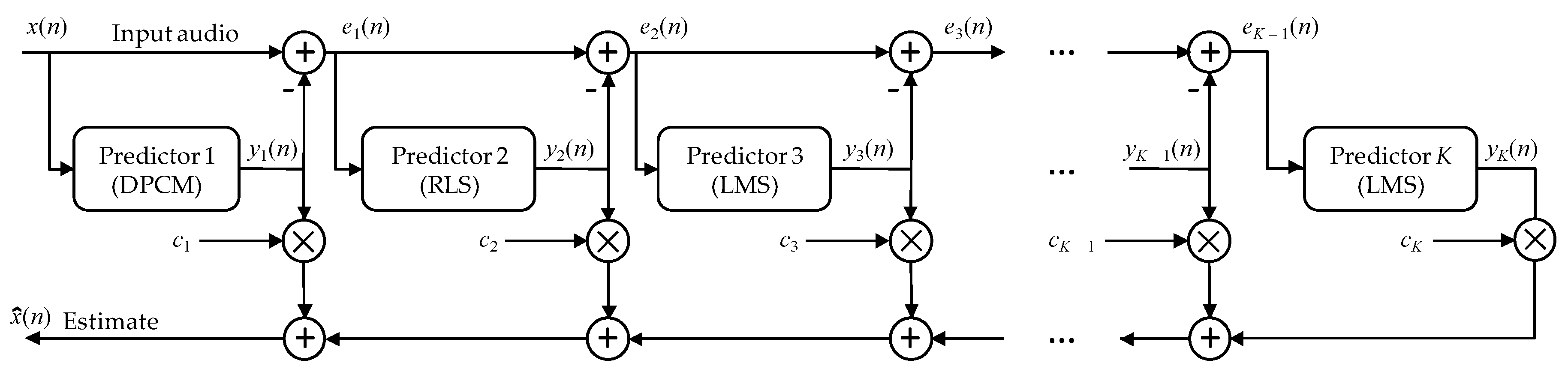
For this reason adaptive versions of codecs are used in practice. Moreover, since the audio data do not constitute a sequence of independent values it is difficult to determine and apply the k-th order of Markov model. In practice, it is assumed that the removal of interdependencies is possible by use of predictive techniques writing only predictive errors into the file. The prediction model can be a linear model of the k-th order or a more complex nonlinear solution, but we reduce it to the one value predicted $\widehat{x}(n)$ (creating not explicitly defined first-order Markov model), which we subtract from the current sample x(n), see Formula (1). As a result a sequence of prediction errors can be interpreted as a source for which the first-order entropy value is noticeably smaller than the zero order entropy (see the third column in Table 3). It should be noted here that it is extremely difficult to determine the total entropy H(S) because it is difficult to determine the order of the Markov model, which will take into account all the interdependencies between the individual data (an example is the use of linear prediction of the order of r = 1000 in the first degree of NLMS proposed here the cascading prediction technique).

Usually, instead of a static Huffman code, the adaptive Rice coder [36] and the multivalued arithmetic coder with quantisation are used for efficient coding of prediction errors [15]. This allows reducing the size of the alphabet as a result of which a part of less-significant bits representing the value of prediction errors is saved without further coding [37]. The method proposed here has a similar implementation complexity compared to the one described in the work [37], where simple mapping function is used. That indicates currently the best Rice code parameter, which corresponds statistically to the most suitable fit (in the medium-term sense) to the distribution used by the coder.

Our solution uses an adaptive Golomb code, whose output data is additionally subjected to compression using two context adaptive binary arithmetic coders (CABAC). Each of these coders has its own way of determining the number of the context with which the individual probability distribution of bits 0 and 1 is associated. This solution is faster than used in work [16] while it is characterised by greater flexibility in adjusting to changes in signal features over time. The combination of adaptive versions of the arithmetic encoder and Golomb code allows for taking into account changes in the characteristics of the probability distribution of prediction errors over in time, which involves into a further decrease the bit average.

7.1. Short-Term Feature of the Probability Distribution

Analysing the closest neighbourhood composed of samples x(n − i) and the prediction error signal e(n − i), the fact that there are short-term dependencies between the coded data in sequence can be used. On the basis of these features, the correct type of distribution of the currently coded modified prediction error $\overline{e}(n)$ value can be determined quite accurately, where $\overline{e}(n)$ = 2e(n) − 1 for e(n) > 0, and $\overline{e}(n)$= −2e(n) in otherwise.

Starting from this assumption, a contextual arithmetic coder is usually designed so that has t distributions of probabilities associated with individual context numbers from 0 to t − 1. Theoretically, it is expected the increase in compression efficiency with the increasing number of contexts. However, there is the problem of too slow adaptation of their distribution to the approximate actual state. The adaptive nature of calculation of probability distributions requires a quick defined of the approximate target shape of each of t distributions. Therefore, a certain compromise should be made between the number of contexts and the speed of adaptation of their distributions. In coding of images t is 8 [33], 16 and even 20 [38].

The proposed solution uses nine classes that define coarse signal characteristics from a short-term point of view, using principles similar to those used in the works [39,40]. The ω parameter is calculated as a weighted average of z = 17 previous prediction error modules |e(n − i)|:

$$\omega =\frac{5}{4z}{\displaystyle \sum _{i=1}^z\frac{\left|e(n-i)\right|}{\sqrt{i}}}.$$

(27)

The ω value is quantised using t − 1 thresholds t_h(j), to obtain the short-term arithmetic context number. For t = 9, thresholds were set as t_h = {4, 10, 30, 50, 80, 180, 500, 1100}, receiving b_medium number belonging to the range $\overline{0;8}$.

It is possible to include ultra-short-term features based on only the closest four errors, by calculating the max{e(n − 1), e(n − 2), e(n − 3), 0.6⋅e(n − 4)} value. If the value is greater than 1500, the b_ultra bit assumes value 1, otherwise 0.

7.2. Medium-Term Features of the Probability Distribution

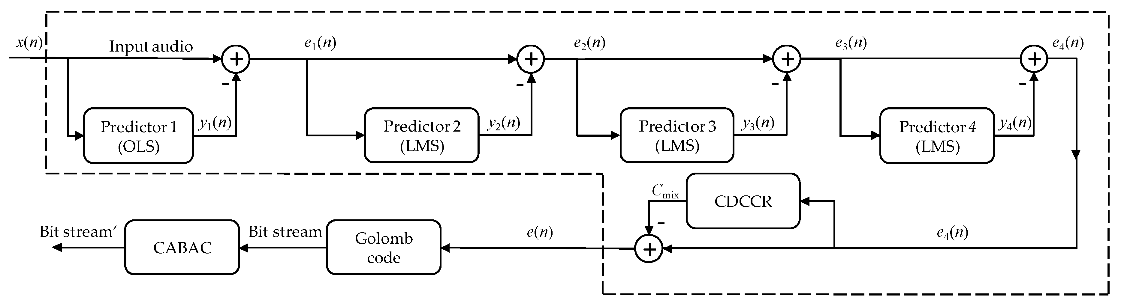
The values of b_medium and b_ultra presented in Section 7.1 provide information on short-term features of the currently estimated probability distribution. Additionally, in the case of the prediction error stream, the assumption is made about the medium-term stationarity of its distribution, which is usually similar to the geometrical distribution. Data on such features can be coded in a highly efficient manner using the Golomb code family [18].

For each coded $\overline{e}(n)$ value, an individual m group number is calculated. For this purpose, the adaptive average cost of coding with the Golomb code use one of the appropriately selected 40 probability distributions. Probability distributions are defined based on the formula G(i) = (1 − p) ⋅ pⁱ, with individual values p_(j) associated with the j-th distribution depending on the m_(j) parameter of the Golomb code, which is the j-th number from the experimentally selected set m = {1, 2, 3, 4, 6, 8, 12, 16, 20, 24, 32, 40, 48, 64, 80, 96, 128, 160, 192, 256, 320, 384, 448, 512, 576, 640, 768, 896, 1024, 1152, 1280, 1536, 1792, 2048, 2560, 3072, 4096, 5120, 6144, 8192}. This increased flexibility gives the Golomb codes an advantage over the Rice code, for which m values can be only a number 2 raised to an integer value (e.g., 2¹ = 2, 2² = 4, 2³ = 8, 2⁴ = 16, …).

To calculate a current predicted value of m, in [17], the estimate using backward adaptation was proposed, applying a local assumption of stationarity S(n), being the average value of modified prediction errors. Assuming that the expected value of modified prediction errors is inversely proportional to 1 − p, we obtain p = (S(n) − 1)/S(n), where the expected value of S(n) equals

$$S(n)=\frac{1}{N_G}{\displaystyle \sum _{i=1}^{N_G}\overline{e}(n-i)},$$

(28)

where N_G specifies the number of previously coded modified prediction errors. The group number m can be calculated using formula presented in [41,42] (at δ = 0):

$$m=\lceil -\frac{{\log }_{10}(1+p)}{{\log }_{10}p}+\delta \rceil .$$

(29)

An experimental correction value δ = 0.41 [17] was introduced to Formula (29) which resulted in a slight decrease in the bit average (for the whole test base). At δ = 0, there is a linear relationship between m and S(n) values of m = (ln 2) ⋅ S(n) [43], and after taking into account δ = 0.41, an approximated form of the formula was determined:

$$m=\lfloor 0.693147\cdot S+0.563636\rfloor .$$

(30)

After simplifying the Formula (28) to the iterative form and using the auxiliary sum S_γ, which is adapted using the formula $S_{\gamma }^{(q)}(n)$ = $\overline{e}(n-1)+{\gamma }_q\cdot S_{\gamma }^{(q)}(n) ,$ we obtain the value of $S^{(q)}(n)$ = $(1-{\gamma }_q)\cdot S_{\gamma }^{(q)}(n).$ The value of γ_q is the experimentally determined forgetting factor, in work [17] it was set at a compromise level of 0.952. A noticeable improvement was obtained by using two forgetting factors (γ₁ = 0.935 and γ₂ = 0.992) and using them to calculate two sums of S⁽¹⁾(n) and S⁽²⁾(n). In addition, we use the weighting effect of these sums, calculating the current average costs L_cost(q) of encoding the input data stream (for q = {1, 2}) using Golomb codes separately for parameters m₁ and m₂:

$$L_{\cos \mathrm{t}(q)}(n)=0.8\cdot L_{\cos \mathrm{t}(q)}(n-1)+lengt{h}_{(q)}(\overline{e}(n)),$$

(31)

which allows calculating weights ${\gamma }_{\cos \mathrm{t}(q)}(n)={0.7}^{L_{\cos \mathrm{t}(q)}(n)}$ necessary to calculate the final value of m:

$$m=\lfloor 0.693147\cdot \frac{{\gamma }_{\cos \mathrm{t}(1)}(n)\cdot S^{(1)}(n)+{\gamma }_{\cos \mathrm{t}(2)}(n)\cdot S^{(2)}(n)}{{\gamma }_{\cos \mathrm{t}(1)}(n)+{\gamma }_{\cos \mathrm{t}(2)}(n)}+0.563636\rfloor ,$$

(32)

which is additionally scaled to best approximate one of the 40 values found in the m vector. The method of scaling is as follows; for m < 1, we assign m = 1 and values between 1 and 6 remain unchanged, whereas for m > 6, we calculate $m:=\lfloor 1.65\cdot m\rfloor$. The last step is the approximation of the calculated m value to the nearest of those in m vector. In this way, the index of the quantised value of m (hereinafter referred to as b_Golomb) is obtained. The b_Golomb value is a fragment of the context number and is invariable when encoding all bits of the next Golomb code word representing the number $\overline{e}(n+1)$.

This allows for a highly flexible adaptation to the local features of the probability distribution of currently coded prediction errors as well as the rate of change of features of this distribution. Then, the quantisation of the m parameter to only 40 values is a compromise approach with regard to the uninterrupted adaptation of each of the 40 probability distributions that are used in the binary arithmetic coder, by which the bit stream coming from Golomb coder is coded.

The Golomb code word coding $\overline{e}(n)$ value consists of two elements. The first one is the $u_G=\lfloor \overline{e}(n)/m\rfloor$ number specifying the group number that is written in the unary form (sequence u_G zeros ending with one). The second element is the $v_G=\overline{e}(n)-u_G\cdot m$ number, called the number of element in a group (remainder of division by m). It is coded using a phased-in binary code (which is the variant of the Huffman code for sources with m equally probable symbols [42]). Specifying the $k=\lceil {\log }_{2}m\rceil$ parameter means that, in each group, the first $l=2^k-m$ elements v_G are coded using k − 1 bits, and the remaining m − l elements are coded as number v_G + l using k bits [13].

7.3. The Way of Determining the Number of Contexts

Binary streams representing u_G and v_G are coded using separate arithmetic coders, with separate ways to determine the context number. The ctx_u context number used to encode the u_G series with zeros terminated with one is calculated for each consecutively coded bit as follows,

ctx_u = 2³⋅(18⋅b_Golomb + 2⋅b_medium + b_ultra) + b_unary

(33)

The b_unary value is a three-bit number (in the range from 0 to 7) specifying the number (counting from the most to the least significant) of the currently coded unary bit of the u_G number. When the bit number is greater than 7 (which takes less than 1% of cases) then b_unary = 7. We therefore obtain 2³⋅18⋅40 = 5760 contexts ctx_u.

In the case of the second coder used to encode the v_G, number, there are slightly fewer contexts, because 2⁴⋅5⋅40 = 3200. The ctx_v number is calculated from the dependency

ctx_v = 2⁴⋅(5⋅b_Golomb + b_phased-in) + 2³⋅b_binary2 + 2²⋅b_binary1 + b_unary2

(34)

where b_unary2 is equal b_unary2 = min{b_unary, 3}. The b_binary1 is the oldest (first in coded order) bit of value v_G. The b_binary2 is the second oldest (second coded) bit of value v_G. Although b_phased-in is a number (in the range from 0 to 4) specifying the number (counting from the more-significant to less-significant bits) of currently coded bits of value v_G, if the bit number is greater than 4, then b_phased-in = 4. Furthermore, when b_phased-in = 0, then b_binary1 = b_binary2 = 0 is set, and if b_phased-in = 1, then b_binary2 = 0.

7.4. Long-Term Adaptation

In the case of an context adaptive binary arithmetic coder with each number of the context, a probability distribution consisting of only two values—p(0) and p(1)—is associated. In practice, the number of occurrences of zeros and ones denoted n(0) and n(1) respectively, then p(0) = n(0)/(n(0) + n(1)), and p(1) = 1 − p(0). The current adaptation of the distribution consists in increasing (in a given context) by 1 counter of occurrences of the currently encoded bit. Additionally, if the total number of occurrences of zeros and ones in a given context exceeds the value of N_max, then their counters n(0) and n(1) are divided by 2, which is the equivalent of the long-term forgetfulness method. For this reason, the designer of such a binary coder should determine both the N_max value and the initial values of n(0) and n(1) within each context in such a way as to obtain the best fit to the encoded data.

In the proposed solution, in all contexts of the u_G coder, N_max = 2⁹ was set, and the counters n(0) and n(1) were initialised with the value 1. In the case of the v_G coder, in all contexts, N_max = 2¹² was set, and the counters were initialised as n(0) = 64 and n(1) = 60.

7.5. Analysis of Practical Aspects of Prediction Error Encoder Implementation

Table 3 presents a comparison of the results for several different encoder settings, using the example of a database containing 16 test files (the average of the whole database was bold in the last row of Table 3). The second column contains the values of H(S_DMS) unconditional entropy here referred to as zero order entropy. The third column contain entropy values of the first-order H(S|C⁽¹⁾) for prediction errors (we are talking about conditional entropy in which according to the first-order Markov model process the context is the predicted value which was calculated using cascade prediction (see Formula (23)). There is a significant decrease (bit average for the whole database of 16 files) from 13.813 to 9.172 bits per sample.

The fourth column takes into account the actual bit average after using our proposed adaptive Golomb; a code described in Section 7.2. This allowed to obtain a bit average lower than H(S|C⁽¹⁾) by 0.407 bits per sample, which shows that predictive modelling is not able to fully remove the mutual information.

On the other hand, the introduction of a block in the form of an context-free arithmetic encoder (with active default long-term adaptation, see Section 7.3), which additionally encodes the stream of bits coming out of the Golomb encoder, allowed for a further decrease of the bit average by another 0.14 bits per sample.

After introducing context rules (medium term adaptation) to the encoder CABAC, the bit average was reduced by 0.082 bits per sample, and after including additional contexts in CABAC (in the short term adaptation, see Section 7.1), the result was improved by reducing the bit average by 0.004 to the target level of 8.539 bits per sample.

8. Schematic Diagram of the Proposed Cascading Audio Data Encoder Method

In Figure 3, the diagram of the target encoder proposed in this work is presented. Although the cascading concept was previously used [24,29] and was considered the most effective way of lossless audio compression, our approach demonstrates that there is scope for further significant improvement within this concept.

In general, we can distinguish two main stages: In the first stage, the prediction value $\widehat{x}(n)$ and prediction error e(n) are calculated (see Formula (23), which was executed by the blocks in the border in the form of a dashed line: OLS+, 3 stages of LMS, CDCCR). The second stage is coding prediction error to binary stream (implemented by Golomb code and CABAC blocks).

Introducing our proposal of OLS+ method to the initial prediction stage allows to remove the interchannel dependencies with the highest correlation with the currently coded sample x(n). The Formula (2) is used here and the method of adaptation of the prediction coefficients described in Section 4.2. The resulting prediction error e₁(n) and previous errors e₁(n − i) contained in the buffer become an input data stream for the next block, which is the first stage of LMS. In LMS1, the dependencies between further samples are removed by linear prediction of the order r₁ = 1000.

Because as an optimised version of adaptive linear prediction (NLMS, see Section 3) with a relatively slow convergent coefficient adaptation procedure (Formula (5)) is used; it cannot fully remove these dependencies. For this reason, this method is used in a cascade manner in two further steps of prediction improvement (using descending orders r₂ = 380 and r₃ = 10), minimising the mean of prediction error. These three LMS blocks use the Formula (20) to calculate consecutive predictive values y₂(n), y₃(n) and y₄(n) and the corresponding prediction errors e₂(n), e₃(n) and e₄(n) obtained from Formula (22).

The last stage in the prediction part is an attempt to remove the context dependent constant component by using our proposal CDCCR method, which has not been widely used in lossless audio compression before. After subtracting from e₄(n), the constant component C_mix calculated from Formula (24), we obtain the final form of the prediction error e(n), which is transmitted to the input of the adaptive Golomb encoder (Section 7.2). This block generates a bit stream, which by use of context dependencies between individual bits is encoded using an arithmetic encoder. In contrast to frequently used multivalue arithmetic encoders, the binary variant of the CABAC adaptive binary encoder is used (see Section 7.3).

The proposed solution is time symmetrical, which means the same complexity is also in case of decoding. The decoding procedure is very similar to the coding stage. In the first two steps (arithmetic decoder and Golomb decoder), the prediction error e(n) must be recovered from the binary stream. This prediction error is added to the predicted value, which is calculated in the same way as in the encoder (see the blocks in the border made by the dashed line in Figure 3), obtaining a decoded sample of x(n). This is a simple transformation of Formula (23) into the following generalised form of the K-step predictive cascade:

$$x(n)=e(n)+\lfloor y_1(n)+y_2(n)+\dots +y_K(n)+C_{\mathrm{mix}}+0.5\rfloor .$$

(35)

Our implementation of the solution proposed here was done in the C language, without considering optimisation of the code or attempts to its parallelisation. However, even with stereo and 44,100 samples per second, it still works online, and the encoding and decoding times are linearly dependent on the number of samples. The encoding program uses one 3.4 GHz i5 processor core in 69.07% (version with ALCM+, see Figure 2) and 93.36% (version with OLS+ block, see Figure 3). In the latter case by dividing the total coding time into blocks we obtain the following proportions: 32.5% − OLS+ block with the order of predictions r = 20, 53.7% − 3 LMS blocks with the total order of predictions r = 1390, 7.5% − CDCCR block. The remaining 6.3% is devoted to the work of blocks: Golomb code, CABAC and for input/output operations.

It is worth noting that the schema of the faster version of the codec proposed here (see Figure 2), in which instead of the OLS+ block the our proposal of ALCM+ method was used with quick adaptation of prediction coefficients, the bit average of 8.667 bits per sample (average for the whole test base) was obtained. This value is lower than in the case of the MP4-ALS-RM23 model in the best mode (8.718 bits per sample, see

Table 4. The bit average of 16 encoded test files using different audio coders.

File	Monkey’s Audio 1	TAK v2.3.0	MP4 2	LA v0.4b	OLS-NLMS [16]	Our Proposition
ATrain	7.441	7.571	7.232	7.204	7.199	7.134
BeautySlept	8.826	8.850	8.305	8.318	8.491	8.265
chanchan	9.938	9.971	9.886	9.782	9.746	9.711
death2	5.930	5.778	6.660	5.907	5.873	5.642
experiencia	11.029	11.153	10.992	10.908	10.911	10.874
female_spech	5.085	4.674	4.710	5.302	4.500	4.493
FloorEssence	9.750	9.841	9.509	9.362	9.355	9.267
ItCouldBeSweet	8.577	8.577	8.396	8.591	8.255	8.307
Layla	9.885	9.943	9.691	9.586	9.633	9.573
LifeShatters	10.874	10.968	10.836	10.777	10.828	10.786
macabre	9.275	9.433	9.076	9.096	9.166	9.082
MaleSpeech	5.221	4.781	4.812	5.233	4.629	4.589
SinceAlways	10.539	10.650	10.473	10.404	10.394	10.377
thear1	11.504	11.622	11.425	11.398	11.435	11.406
TomsDiner	7.423	7.341	7.268	7.153	7.116	7.114
velvet	10.508	10.314	10.212	10.248	10.029	9.999
Bit average	8.863	8.842	8.718	8.704	8.597	8.539

¹ Monkey’s Audio in version 4.33, ² MP4-ALS-RM23 in the best mode.

) using RLS block of higher implementation complexity than in the case of ALCM+. For more comparisons with other existing publicly available codecs see Section 9.

9. Experimental Research

Sixteen fragments of recordings (various genres of music as well as men’s and women’s speech recordings) were used to perform efficiency analysis. The recordings are long for several seconds, and all available in the database [44]. Comparing to the bit average of the general purpose coder RAR v5.0, our solution achieves as much as 21.08% better result, because the bit average of compressed the same test base using RAR equal 10.82. The result of the encoding of these recordings by the proposed method is presented in Table 4 and

Table 5. The bit average of 16 encoded test files using different audio coders.

File	Shorten v3.6.1	TTA v3.4.1	MP4 1	FLAC v1.3.2	WavPack v4.60.1	Nanozip v0.09a
ATrain	8.637	8.189	7.862	7.933	7.792	7.396
BeautySlept	10.724	10.188	10.049	10.005	9.825	8.671
chanchan	10.863	10.077	10.160	10.127	10.032	9.980
death2	7.152	6.306	6.496	6.284	6.620	5.982
experiencia	12.290	11.334	11.377	11.371	11.252	11.099
female_spech	7.539	5.267	5.242	5.329	5.204	5.048
FloorEssence	11.464	10.176	10.202	10.174	9.922	9.677
ItCouldBeSweet	11.587	9.186	9.016	9.004	8.858	8.776
Layla	10.871	10.300	10.377	10.344	10.202	9.859
LifeShatters	12.177	11.145	11.182	11.146	11.052	10.927
macabre	10.564	10.062	9.965	9.895	9.928	9.267
MaleSpeech	7.532	5.530	5.590	5.649	5.333	5.024
SinceAlways	12.192	11.243	11.164	11.211	10.749	10.564
thear1	12.574	11.703	11.742	11.746	11.635	11.685
TomsDiner	9.709	8.561	8.534	8.404	8.087	7.480
velvet	11.067	11.464	10.672	10.679	10.843	10.656
Bit average	10.434	9.421	9.352	9.331	9.208	8.881

¹ MP4-ALS-RM23 in default mode.

, where the results of other effective available audio coders are also included (the best results for the individual files in Table 4 are underlined, the bit average of the whole database was bold in the last row of Table 4 and Table 5). The bit average obtained after coding proposed in this work using the multistage OLS+/NLMS method was the lowest of all coders listed in the table. The propose method had an 8.7% lower bit average than obtained using the MP4-ALS-RM23 method (default mode), and also had a 2.1% lower bit average compared to MP4-ALS-RM23 using the best mode.

10. Conclusions

This work presents an extended version of the cascading audio data encoder. In classic solutions of lossless audio coding, adaptive versions of Rice and arithmetic encoders are used interchangeably. The proposed solution uses an adaptive Golomb code, which is a generalised form of the Rice code with potentially higher compression efficiency because of a better adaptation of the code to the current probability distribution of the currently encoding data. The Golomb codec output is additionally compressed using a context-dependent adaptive binary arithmetic encoder. In contrast to CABAC [45], where the Exp-Golomb distribution is used, our proposition adapts better to the sequence of prediction errors characterised by the geometric distribution.

The proposed adaptive arithmetic coder presented in this paper offers less computational complexity compared to the coder used in the work [16]. A higher degree of compression was obtained due to a better algorithm for selection of context numbers, and also due to the omission a multivalued arithmetic coder in favour a binary variant (this allows increasing the dynamics adaptation to probability distributions of individual bits of values u_G and v_G calculated in the Golomb encoder block). This solution is more flexible also in comparison to classic solutions using the adaptive Rice code.

In the proposed solution, the increase in efficiency of compression compared to the most efficient option MP4-ALS-RM23 (working in backward adaptation mode) was possible due to introducing a more efficient OLS+ block in place of RLS, adding an additional CDCCR block in the cascaded predictive model and introducing an efficient CABAC based on initial compression using the adaptive Golomb code. The introduced improvements entail a disproportionately large increase in the implementation complexity relative to the reference version, for which was adopted MP4-ALS-RM23 in the best mode. Despite the increasing implementation complexity it has been kept at a level enabling real-time encoding and decoding. Similar conclusions can also be drawn by comparing the reference version (the best mode) with the MP4-ALS-RM23 in default mode. Therefore, one should be aware that shortening the length of the result files for each subsequent percentage is paid by the increasing costs of increasing the implementation complexity. This is similar to the nonlinear increase in energy necessary to speed up objects that want to approach the speed of light in vacuo. The complexity of an efficient cascade prediction system also is possible to reduce by regulation not only by modifying the orders of predictive models in NLMS blocks. We propose using the ALCM+ block with a much lower implementation complexity compared to RLS and OLS+ blocks.

References

1. The Moving Picture Experts Group Homepage. Available online: https://mpeg.chiariglione.org/ (accessed on 28 April 2019).
2. Liebchen, T.; Reznik, Y.A. Improved Forward-Adaptive Prediction for MPEG-4 Audio Lossless Coding. In Proceedings of the 118th AES Convention, Barcelona, Spain, 28–31 May 2005; pp. 1–10. [Google Scholar]
3. Andriani, S.; Calvagno, G.; Erseghe, T.; Mian, G.A.; Durigon, M.; Rinaldo, R.; Knee, M.; Walland, P.; Koppetz, M. Comparison of lossy to lossless compression techniques for digital cinema. In Proceedings of the International Conference on Image Processing ICIP’04, Singapore, 24–27 October 2004; Volume 1, pp. 513–516. [Google Scholar]
4. Monkey’s Audio Codec Homepage. Available online: http://www.monkeysaudio.com/ (accessed on 28 April 2019).
5. Free Lossless Audio Codec Homepage. Available online: https://www.xiph.org/flac (accessed on 28 April 2019).
6. Robinson, T. SHORTEN: Simple Lossless and Near-Lossless Waveform Compression; Technical report 156; Cambridge University Engineering Department: Cambridge, UK, 1994; pp. 1–17. [Google Scholar]
7. Hybrid Lossless Audio Compression Homepage. Available online: http://wavpack.com/ (accessed on 12 October 2019).
8. NanoZip Experimental File Archiver Software Homepage. Available online: http://nanozip.ijat.my/ (accessed on 1 October 2019).
9. TTA Lossless Audio Codec Overview Homepage. Available online: http://tausoft.org/wiki/True_Audio_Codec_Overview (accessed on 12 October 2019).
10. Tom’s lossless Audio Kompressor (TAK) Codec Homepage. Available online: http://thbeck.de/Tak/Tak.html (accessed on 12 October 2019).
11. Lossless Audio (LA) Compression Program Homepage. Available online: http://www.lossless-audio.com/ (accessed on 14 October 2019).
12. Coding of Audio-Visual Objects ISO Standard Homepage. Available online: https://www.iso.org/standard/53943.html (accessed on 28 April 2019).
13. Sayood, K. Introduction to Data Compression, 5th ed.; Morgan Kaufmann Publishers/Elsevier: Cambridge, MA, USA, 2018. [Google Scholar]
14. Wernik, C.; Ulacha, G. Analysis of inter-channel dependencies in audio lossless block coding. In Proceedings of the Federated Conference on Computer Science and Information Systems (FedCSIS), Poznań, Poland, 9 September 2018; pp. 135–139. [Google Scholar]
15. Ulacha, G.; Stasiński, R. Lossless Audio Coding by Predictor Blending. In Proceedings of the 36th International Conference on Telecommunications and Signal Processing (TSP), Rome, Italy, 2–4 July 2013; pp. 502–506. [Google Scholar]
16. Ulacha, G.; Stasiński, R. Entropy coder for audio signals. Int. J. Electron. Telecommun. 2015, 61, 219–224. [Google Scholar] [CrossRef]
17. Wernik, C.; Ulacha, G. Application of adaptive Golomb codes for lossless audio compression. In Proceedings of the 23rd Conference Signal Processing: Algorithms, Architectures, Arrangements, and Applications (SPA), Poznań, Poland, 19–20 September 2018; pp. 203–207. [Google Scholar]
18. Golomb, S.W. Run-length encoding. IEEE Trans. Inf. Theory 1966, 12, 399–401. [Google Scholar] [CrossRef]
19. Moriya, T.; Yang, D.; Liebchen, T. Extended Linear Prediction Tools for Lossless Audio Coding. In Proceedings of the IEEE International Conference on Acoustics, Speech, and Signal Processing (ICASSP’04), Montreal, QC, Canada, 17–21 May 2004; Volume 3, pp. 1008–1011. [Google Scholar]
20. Ghido, F.; Tabus, I. Sparse Modeling for Lossless Audio Compression. IEEE Trans. Audio Speech Lang. Process. 2013, 21, 14–28. [Google Scholar] [CrossRef]
21. Biswas, A.; den Brinker, B. Lossless compression of digital audio using Laguerre-based pure linear prediction. In Proceedings of the SPS 2004 (4th IEEE Benelux Signal Processing Symposium), Hilvarenbeek, The Netherlands, 15–16 April 2004; pp. 49–52. [Google Scholar]
22. Wernik, C.; Ulacha, G. Audio lossless encoding with adaptive Context-Dependent Constant Component Removing. In Proceedings of the 27th International Conference on Software, Telecommunications and Computer Networks (SoftCOM), Split, Croatia, 19–21 September 2019. [Google Scholar]
23. Saeed, V. Vaseghi Advanced Digital Signal Processing and Noise Reduction, 2nd ed.; John Wiley & Sons Ltd.: Hoboken, NJ, USA, 2000; pp. 228–262. ISBN 0-471-62692-9. [Google Scholar]
24. Huang, H.; Fränti, P.; Huang, D.; Rahardja, S. Cascaded RLS-LMS prediction in MPEG-4 lossless audio coding. IEEE Trans. Audio Speech Lang. Process. 2008, 16, 554–562. [Google Scholar] [CrossRef]
25. Ravelli, E.; Gournay, P.; Lefebvre, R. A Two-Stage MLP+NLMS Lossless coder for stereo audio. In Proceedings of the IEEE International Conference on Acoustics, Speech, and Signal Processing (ICASSP’06), Toulouse, France, 14–19 May 2006; Volume 5, pp. 177–180. [Google Scholar]
26. Makino, S.; Kaneda, Y.; Koizumi, N. Exponentially weighted stepsize NLMS adaptive filter based on the statistics of a room impulse response. IEEE Trans. Speech Audio Process. 1993, 1, 101–108. [Google Scholar] [CrossRef]
27. Sayood, K. Lossless Compression Handbook; Academic Press: San Diego, CA, USA, 2003. [Google Scholar]
28. Hoerl, A.E.; Kennard, R.W. Ridge Regression: Biased Estimation for Nonorthogonal Problems. Technometrics 1970, 12, 55–67. [Google Scholar] [CrossRef]
29. Huang, H.; Rahardja, S.; Lin, X.; Yu, R.; Fränti, P. Cascaded RLS-LMS prediction in MPEG-4 lossless audio coding. In Proceedings of the International Conference on Acoustics, Speech and Signal Processing (ICASSP 2006), Toulouse, France, 14–19 May 2006; Volume 5, pp. 181–184. [Google Scholar]
30. Ulacha, G.; Stasiński, R. Performance Optimized Predictor Blending Technique for Lossless Image Coding. In Proceedings of the 36th International Conference on Acoustics, Speech and Signal Processing ICASSP’11, Prague, Czech Republic, 22–27 June 2011; pp. 1541–1544. [Google Scholar]
31. Ye, H.; Deng, G.; Devlin, J.C. Adaptive linear prediction for lossless coding of greyscale images. In Proceedings of the IEEE International Conference on Image Processing (CDROM), Vancouver, BC, Canada, 10–13 September 2000. [Google Scholar]
32. Ulacha, G.; Stasiński, R. Context based lossless coder based on RLS predictor adaptation scheme. In Proceedings of the International Conference on Image Processing ICIP 2009, Cairo, Egypt, 7–10 November 2009; pp. 1917–1920. [Google Scholar]
33. Wu, X.; Memon, N.D. CALIC-A Context Based Adaptive Lossless Image Coding Scheme. IEEE Trans. Commun. 1996, 45, 437–444. [Google Scholar] [CrossRef]
34. Weinberger, M.J.; Seroussi, G.; Sapiro, G. LOCO-I Lossless Image Compression Algorithm: Principles and Standardization into JPEG-LS. IEEE Trans. Image Process. 2000, 9, 1309–1324. [Google Scholar] [CrossRef] [PubMed]
35. Topal, C.; Gerek, Ö.N. Pdf sharpening for multichannel predictive coders. In Proceedings of the 14th European Signal Processing Conference (EUSIPCO-06), Florence, Italy, 4–8 September 2006. [Google Scholar]
36. Rice, R.F. Some Practical Universal Noiseless Coding Techniques; JPL Publication 79-22; Jet Propulsion Labolatory: Pasadena, CA, USA, March 1979. [Google Scholar]
37. Reznik, Y.A. Coding of prediction residual in MPEG-4 standard for lossless audio coding (MPEG-4 ALS). In Proceedings of the IEEE International Conference on Acoustics, Speech, and Signal Processing (ICASSP’04), Montreal, QC, Canada, 17–21 May 2004; Volume 3, pp. 1024–1027. [Google Scholar]
38. Deng, G.; Ye, H. Lossless image compression using adaptive predictor combination, symbol mapping and context filtering. In Proceedings of the IEEE 1999 International Conference on Image Processing, Kobe, Japan, 24–28 October 1999; Volume 4, pp. 63–67. [Google Scholar]
39. Aiazzi, B.; Alparone, L.; Baronti, S. Context modeling for nearlossless image coding. IEEE Signal Process. Lett. 2002, 9, 77–80. [Google Scholar] [CrossRef]
40. Matsuda, I.; Ozaki, N.; Umezu, Y.; Itoh, S. Lossless coding using Variable Blok-Size adaptive prediction optimized for each image. In Proceedings of the 13th European Signal Processing Conference EUSIPCO-05 CD, Antalya, Turkey, 4–8 September 2005. [Google Scholar]
41. Bhaskaran, V.; Konstantinides, K. Image and Video Compression Standards: Algorithms and Architectures, 2nd ed.; Kluwer Academic Publishers: Palo Alto, CA, USA, 1997. [Google Scholar]
42. Salomon, D. Data Compression: The Complete Reference, 3rd ed.; Springer-Verlag as part of Springer Science & Business Media: New York, NY, USA, 2004. [Google Scholar]
43. Sugiura, R.; Kamamoto, Y.; Harada, N.; Moriya, T. Optimal Golomb-Rice Code Extension for Lossless Coding of Low-Entropy Exponentially Distributed Sources. IEEE Trans. Inf. Theory 2018, 64, 3153–3161. [Google Scholar] [CrossRef]
44. Test Database. Available online: http://www.rarewares.org/test_samples/ (accessed on 28 April 2019).
45. Thiele, C.C.; Vizzotto, B.B.; Martins, A.L.M.; da Rosa, V.S.; Bampi, S. A low-cost and high efficiency entropy encoder architecture for H.264/AVC. In Proceedings of the 2012 IEEE/IFIP 20th International Conference on VLSI and System-on-Chip (VLSI-SoC), Santa Cruz, CA, USA, 7–10 October 2012; pp. 117–122. [Google Scholar]
Figure 1. Cascaded RLS-LMS prediction in MPEG-4 lossless audio coding [24,29].
Applsci 09 05218 g001
Figure 2. Schema of our approach for lossless audio coding.
Applsci 09 05218 g002
Figure 3. Schema of our approach for lossless audio coding.
Applsci 09 05218 g003