Mixed-Unit Lattice Approach for Area Determination of Cellular and Subcellular Structures

Department of Mathematics, Elwood John Glenn, Elwood, NY 11731, USA
Appl. Sci. 2019, 9(24), 5267; https://doi.org/10.3390/app9245267
Submission received: 14 November 2019
/
Revised: 29 November 2019
/
Accepted: 30 November 2019
/
Published: 4 December 2019
(This article belongs to the Section Applied Biosciences and Bioengineering)
Abstract
:Featured Application
Presented herein is a novel method for determining the areas of cellular and subcellular structures including renal cysts and glomeruli. Use of this mixed unit lattice outperforms the conventional method used for these measurements. Accurate determination of cellular and subcellular dimensions is critical to detect changes therein, changes that often alert to ongoing disease.
Abstract
Even small changes in the dimensions of cellular and subcellular structures can inform an ongoing disease. An increase in glomerular dimensions is associated with kidney disease and can predict glomerulosclerosis, whereas an increase in the size of fluid-filled renal cysts is predictive of end-stage polycystic kidney disease. In the absence of set formulae to define the area of curvilinear irregular regions, such as glomeruli and cysts, the method of counting unit squares is used. Nonetheless, as infinitesimally small as the unit square may be, this 2D space-filling method still underestimates the area of a curvilinear region. Developed herein is a mixed-unit lattice approach that represents an improvement over the existing method for estimating the areas of cellular and subcellular structures. In test cases comprising images of glomeruli and renal cysts, this method outperformed the conventional unit-squares method, and may form the foundation for refining the current method used by most types of software for estimating the area of irregular curvilinear regions.
1. Introduction
The area determination of cellular and subcellular structures, including glomeruli and renal cysts, is important in that it can signify the status of an ongoing disease. Kidney diseases can be associated with glomerular hypertrophy or expansion, both in nonclinical models and in patients [1,2]. In fact, glomerular expansion is predictive of a relapse in minimal change disease (MCD) and progression in glomerular scarring [2,3]. In patients with focal segmental glomerulosclerosis (FSGS), an increase in glomerular dimensions is directly associated with rapid progression to end-stage renal disease [4]. In polycystic kidney disease (PKD), cyst expansion drives an increase in renal dimensions, which, in turn, precipitates organ dysfunction [5]. Serial determination of changes in the glomerular area and cystic index can thus inform of both the presence and progress of renal disease. In nonclinical models, measurement of these continuous variables can inform of test article efficacy.
Currently used software for the planimetric determination of surface areas calculates the area of shapes by counting unit squares or pixels [6,7]. The software works by scanning the image until it finds the edge of an object, outlines or defines the object, and then populates the interior with unit square pixels, i.e., pixels that have equal horizontal (width) and vertical (length) sampling pitch of 1. The area of the curvilinear region, i.e., pixel area x number of pixels, can be assigned a real value by using a calibration tool. Due to the inherent properties of the curvilinear shape of cellular and subcellular bodies, such as glomeruli and cysts, square pixels do not populate every aspect of the curvilinear region, especially along the edges of the image. Consequently, the true area is underestimated more often than not.
Here, we present novel method to calculate the areas of curvilinear shapes. This method relies on introducing more vertices into the unit shapes by utilizing a mixed lattice comprising unit hexagons and unit triangles.
2. Materials and Methods
2.1. Area Determination of Curvilinear Regions, Glomeruli, and Renal Cysts
A circle and a curvilinear plane were drawn using GeoGebra. Banked slides of rat kidneys (kindly provided by Angion Biomedica Corp., Uniondale, NY, USA, institutional approval #2016-004) were photographed and used in the current study. Glomeruli (n = 4) from periodic acid Schiff (PAS)-stained adult male Sprague-Dawley rat-kidney sections were photographed at 40× magnification. Renal cysts (n = 5) from Masson’s Trichrome-stained kidneys of adult male PCK rats were photographed at 10×. Areas of the circle, curvilinear plane, renal cysts, and glomeruli were measured by importing images into ImageJ. A slide (AmScope) containing 0.01 mm wide divisions was photographed at 40× and 10× for calibration purposes. For our method of counting unit squares, images were imported into GeoGebra and populated with unit squares, with the length of each side being 1, and an area of
Only squares fully enclosed within the boundaries of the test regions were counted. Using GeoGebra, images were also populated with a mixed lattice comprising unit hexagons, each with a side length of 1 and an area of
and unit triangles, each with a side length of 1 and an area of
The hexagons were filled in first, and the remaining space was populated with triangles. Only hexagons and triangles fully enclosed within the boundaries of the test regions were counted.
2.2. Data Analysis
The gold-standard area of any given region was obtained using ImageJ, which uses a unit square pixel typically of 0.26 mm length and width each. The square and mixed-unit lattices had much greater side length than that of a pixel; consequently, areas calculated using either of these methods were smaller than those obtained with ImageJ. The percentage improvement of the mixed-unit lattice method over the unit-square method was determined, and a two-tailed T-test was used to test the hypothesis that the usage of a mixed-unit lattice would return areas larger than those obtained using unit squares for glomeruli and the renal cysts.
3. Results
As seen in Figure 1A, a circle of a 6 unit radius and an area of 113.1 unit2 were calculated via the area formula for a circle. Use of ImageJ to measure the area of the circle yielded a value of 112.3 unit2. Populating this circle with unit squares (Figure 1B) and counting the number of squares lying within the circle yielded a measured area of 88 unit2. On the other hand, populating this circle with a mixed lattice comprising hexagons and triangles and then counting the total number that were within the circle yielded a measured area of 93.5 unit2.
By contrast to the circle shown in Figure 1, there was no preset formula to calculate the area of the arbitrary irregular curvilinear region shown in Figure 2A. Use of ImageJ to measure this area yielded 87.3 unit2. Populating this region with unit squares (Figure 2B) and counting their number yielded a calculated area of 72 unit2. Use of the mixed-unit lattice approach (Figure 2C) yielded a calculated area of 74.4 unit2.
Next, areas of several glomeruli and renal cysts were calculated using the unit-squares and the mixed-unit lattice methods, and results were compared with the areas obtained using ImageJ.
An image of a glomerulus, as seen in Figure 3A, was populated with either unit squares (Figure 3B) or the mixed-unit lattice (Figure 3C). Areas of a number of glomeruli were measured using ImageJ and then calculated. As seen in Table 1, in each case, the mixed-unit lattice returned a value closer to that measured by ImageJ, and it outperformed the unit squares method (p < 0.01).
An image of a renal cyst, as seen in Figure 4A, was populated with either unit squares (Figure 4B) or the mixed-unit lattice (Figure 4C). Areas of a number of renal cysts were measured and calculated. As seen in Table 2, in each case the mixed-unit lattice returned a value closer to that measured by ImageJ and outperformed the unit-squares method (p < 0.01).
In each of the above instances, the area of the region measured using ImageJ was substantially greater than that when using either the unit-squares method or the mixed-unit lattice method. A better approximation to the ImageJ values could be made by shrinking the physical size of the unit square or the mixed-unit lattice, akin to shrinking a segment of 1 in length to 1 cm or 1 mm. Use of ImageJ to measure the cyst area, as seen in Figure 5, yielded an area of 68.8 unit2. Calculating its areas using larger unit squares (Figure 5B) yielded a value of 46 unit2, whereas the use of smaller unit squares (Figure 5C) yielded an area of 58 unit2. Use of the mixed but large unit lattice (Figure 5D) yielded a calculated area of 52.8 unit2, whereas use of a mixed smaller unit lattice (Figure 5E) yielded 63.8 unit2, a value approaching that measured using ImageJ.
4. Discussion
In this study, we outlined a developed mixed-unit lattice comprising hexagons and triangles that outperformed the conventional unit squares or pixels method in determining the area of curvilinear regions. The mixed-unit lattice method proved superior to the unit-squares method in determining the areas of biological ultrastructures, including glomeruli and renal cysts.
Changes in the dimensions of cells and subcellular structures could be associated with a number of diseases [8,9]. Cardiomyocyte hypertrophy occurs during ventricular remodeling and could signal cardiomyopathy [10], and glomeruli hypertrophy can occur in kidney disease. Both adriamycin- and puromycin-induced models of proteinuric kidney disease are accompanied by glomerular hypertrophy, with the amount of urine protein proportional to the extent of glomerular remodeling [1,11]. In fact, the extent of glomerular expansion informs a number of clinical outcomes, including risk of relapse in MCD, and the risk of transition from MCD to FSGS [2,3,4,12]. Both glomerular size and the number of hypertrophied glomeruli are biomarkers for progression to end-stage renal disease [1].
Availability of serial biopsies in the setting of proteinuric kidney disease makes the determination of glomerular changes possible. Given that, in many mammalian models, glomerular diameters are of the order of 50 to 70 μm with even a 10% increase in glomerular dimensions assuming significance, accurate determination of the glomerular area and changes therein is critical [1]. In PKD, expansion of fluid-filled cysts drives an increase in total kidney volume (TKV) [5]. A number of studies [13,14,15] have shown that increasing TKV corresponds to a more rapid decline in renal dysfunction. Measurement of the cystic index (i.e., the ratio of cystic area or cystic volume to renal parenchymal area or TKV, respectively) is critical to inform of disease progression [5]. Furthermore, at least in preclinical PKD models, the efficacy of a number of therapeutic strategies is determined by the ability of these regimens to retard the progressive increase in cystic index [13,14,15]. Measurement of the cystic area and time-dependent changes therein is therefore critical to inform of both disease status and drug efficacy.
Cellular and subcellular bodies rarely assume well-defined geometric shapes that lend themselves to the easy calculation of their cross-sectional areas. More often than not, their cross-sectional areas are curvilinear regions. Planimetric techniques currently use the method of counting the number of unit squares lying within a region of interest to estimate this area [6,7]. Nonetheless, given the inherent shape of a square vs. that of a curvilinear plane, there is often underestimation of the region’s true area. Reported herein is an improvised solution for the same via use of a mixed lattice method comprising unit hexagons and unit triangles.
Across a wide variety of curvilinear shapes, including a circle, a randomly drawn figure, glomeruli, and renal cysts, the mixed-unit lattice method outperformed the conventional unit-squares method. In fact, after shrinking the size of the unit segment, performance of the mixed-unit lattice approached that of the ImageJ method, which utilizes multifold smaller unit squares or pixels to determine areas. It can be inferred that shrinking the size of the unit hexagon and the unit triangle down to that of a pixel further improves area-measurement accuracy.
The greater the number of its vertices, the better the calculation of the approximate area of a given geometric shape inscribed within a circle [16]. Given a square whose four corners lie in a circle, and an equilateral triangle whose three corners also lie in that circle, the square far better approximates the area of that circle than the triangle. By contrast, an n-sided polygon whose vertices lie in that circle approximates the area of that circle the closest, with increasing n [16].
The mixed-unit lattice described above employed a solution of hexagons and triangles that reduces the penalty on operating systems when calculating the approximate area of curvilinear regions. More complex mixed lattices, such as those comprising polygons, circles, and triangles, may certainly prove superior to the one described herein. Nevertheless, our work represents proof of- concept of a method superior to the traditional method of informing of microscopic biological structure areas on slides, and forms the foundation for refining the current method used by most types of software for estimating the area of irregular curvilinear regions.
5. Conclusions
Quantification of subtle changes in cellular and subcellular dimensions informs of disease status, disease prognosis, and the effectiveness of related therapies. Reducing the mixed-unit lattice method can, in practice, better inform of critical changes in biological structures.
Author Contributions
Conceptualization, R.N.; methodology, R.N.; formal analysis, R.N.; writing, R.N.
Funding
This research received no external funding.
Conflicts of Interest
The authors declare no conflict of interest.
References
- Liu, M.; Goldberg, I.D.; Narayan, P. Glomerular Remodeling in Proteinuric Kidney Disease. J. Am. Soc. Nephrol. 2019, 30, SA-PO0582. [Google Scholar]
- Lee, S.W.; Yu, M.Y.; Baek, S.H.; Ahn, S.Y.; Kim, S.; Na, K.Y.; Chae, D.W.; Chin, H.J. Glomerular Hypertrophy Is a Risk Factor for Relapse in Minimal Change Disease Patients. Nephron 2016, 132, 43–50. [Google Scholar] [CrossRef] [PubMed]
- Fogo, A.; Hawkins, E.P.; Berry, P.L.; Glick, A.D.; Chiang, M.L.; MacDonell, R.C., Jr.; Ichikawa, I. Glomerular hypertrophy in minimal change disease predicts subsequent progression to focal glomerular sclerosis. Kidney Int. 1990, 38, 115–123. [Google Scholar] [CrossRef] [PubMed] [Green Version]
- Hughson, M.D.; Puelles, V.D.; Hoy, W.E.; Douglas-Denton, R.N.; Mott, S.A.; Bertram, J.F. Hypertension, glomerular hypertrophy and nephrosclerosis: The effect of race. Nephrol. Dial. Transpl. 2014, 29, 1399–1409. [Google Scholar] [CrossRef] [PubMed] [Green Version]
- Nieto, J.A.; Yamin, M.A.; Goldberg, I.D.; Narayan, P. An Empirical Biomarker-Based Calculator for Cystic Index in a Model of Autosomal Recessive Polycystic Kidney Disease-The Nieto-Narayan Formula. PLoS ONE 2016, 11, e0163063. [Google Scholar] [CrossRef] [PubMed] [Green Version]
- Available online: https://www.woundsresearch.com/article/histogram-planimetry-method-measurement-irregular-wounds (accessed on 11 November 2019).
- Available online: https://imagej.nih.gov/ij/ (accessed on 11 November 2019).
- Chao, K.; Liao, K.; Khan, M.; Shi, C.; Li, J.; Goldberg, I.D.; Narayan, P. An Improved Method for Estimating Renal Dimensions; Implications for Management of Kidney Disease. Appl. Sci. 2019, 9, 3198. [Google Scholar] [CrossRef] [Green Version]
- Nieto, J.A.; Zhu, J.; Duan, B.; Li, J.; Zhou, P.; Paka, L.; Yamin, M.A.; Goldberg, I.D.; Narayan, P. A modified elliptical formula to estimate kidney collagen content in a model of chronic kidney disease. PLoS ONE 2018, 13, e0190815. [Google Scholar] [CrossRef] [PubMed] [Green Version]
- Olivetti, G.; Melissari, M.; Balbi, T.; Quaini, F.; Cigola, E.; Sonnenblick, E.H.; Anversa, P. Myocyte cellular hypertrophy is responsible for ventricular remodelling in the hypertrophied heart of middle aged individuals in the absence of cardiac failure. Cardiovasc. Res. 1994, 28, 1199–1208. [Google Scholar] [CrossRef] [PubMed] [Green Version]
- Fries, J.W.; Sandstrom, D.J.; Meyer, T.W.; Rennke, R.G. Glomerular hypertrophy and epithelial cell injury modulate progressive glomerulosclerosis in the rat. Lab. Investig. 1989, 60, 205–218. [Google Scholar] [PubMed]
- Nishimoto, K.; Shiiki, H.; Nishino, T.; Uyama, H.; Iwano, M.; Dohi, K. Reversible glomerular hypertrophy in adult patients with primary focal segmental glomerulosclerosis. J. Am. Soc. Nephrol. 1997, 8, 1668–1678. [Google Scholar] [PubMed]
- Irazabal, M.V.; Mishra, P.K.; Torres, V.E.; Macura, S.I. Use of Ultra-high Field MRI in Small Rodent Models of Polycystic Kidney Disease for In Vivo Phenotyping and Drug Monitoring. J. Vis. Exp. 2015, 23, e52757. [Google Scholar] [CrossRef] [PubMed] [Green Version]
- Corradi, V.; Gastaldon, F.; Caprara, C.; Giuliani, A.; Martino, F.; Ferrari, F.; Ronco, C. Predictors of rapid disease progression in autosomal dominant polycystic kidney disease. Minerva Med. 2017, 108, 43–56. [Google Scholar] [PubMed]
- Ta, M.H.; Schwensen, K.G.; Foster, S.; Korgaonkar, M.; Ozimek-Kulik, J.E.; Phillips, J.K.; Peduto, A.; Rangan, G.K. Effects of TORC1 Inhibition during the Early and Established Phases of Polycystic Kidney Disease. PLoS ONE 2016, 11, e0164193. [Google Scholar] [CrossRef]
- Available online: https://www.maa.org/external_archive/joma/Volume7/Aktumen/Polygon.html (accessed on 11 November 2019).
Figure 1.
Area of a circle. (A) Circle of radius 6. (B) Circle populated with unit squares. Blue but not pink, squares were completely enclosed within circle and counted. (C) Circle populated with lattice comprising unit hexagons and unit triangles. Hexagons were filled in first, and then triangles.

Figure 2.
Area of irregular curvilinear region. (A) Region of interest (outlined in black). (B) Region populated with unit squares. Blue but not pink squares were completely enclosed within region and counted. (C) Region populated with lattice comprising unit hexagons and unit triangles. Hexagons were filled in first, then triangles (green). Pink triangles lay outside the region and were not counted.
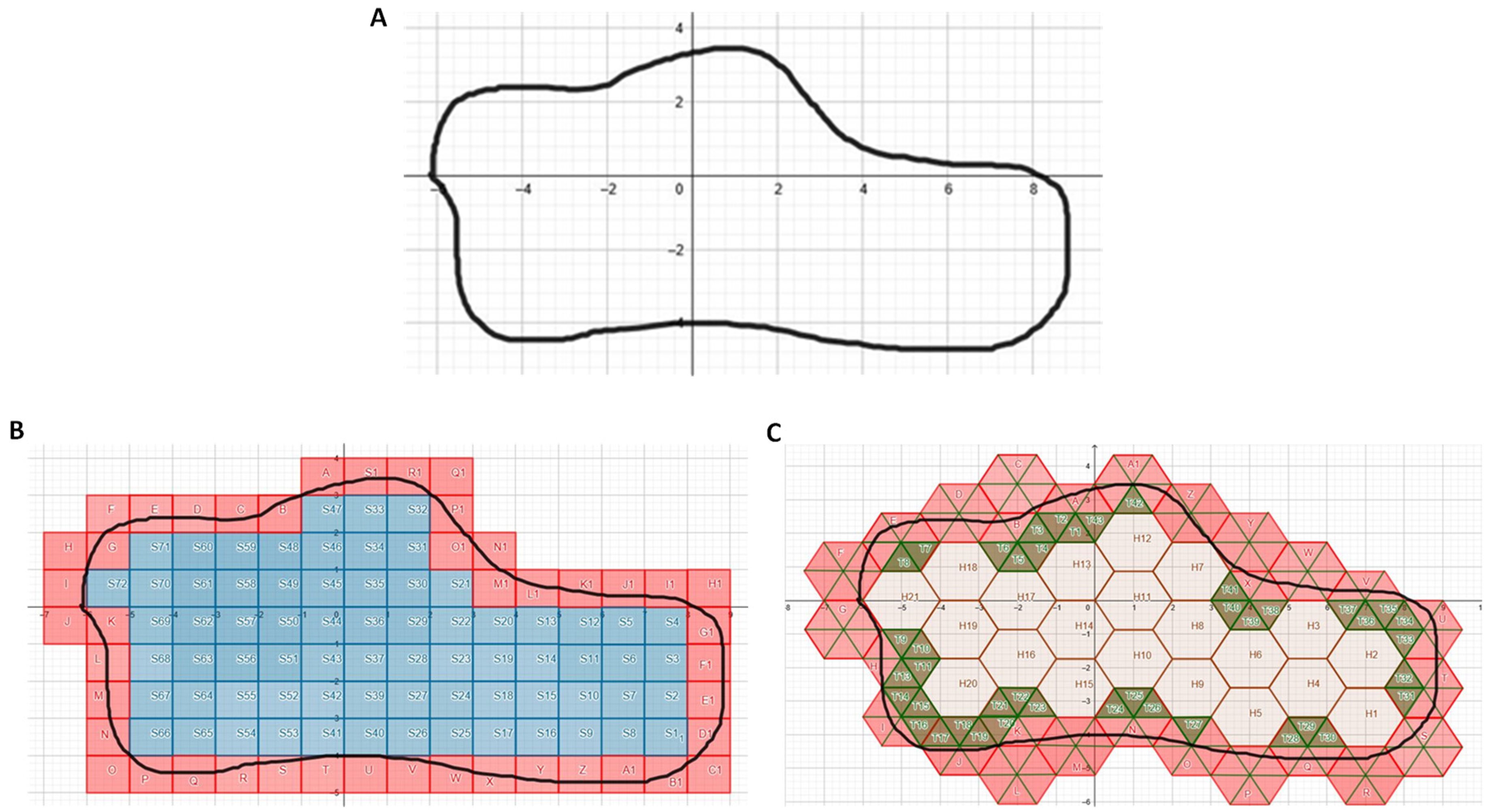
Figure 3.
Area of a glomerulus. (A) Region of interest (outlined by pink line). (B) Region populated with unit squares. Only blue/turquoise squares were completely enclosed within the region and counted. (C) Region populated with lattice comprising unit hexagons and unit triangles. Hexagons were filled in first, then triangles (green). All hexagons and green triangles lay within region of interest and were therefore counted.
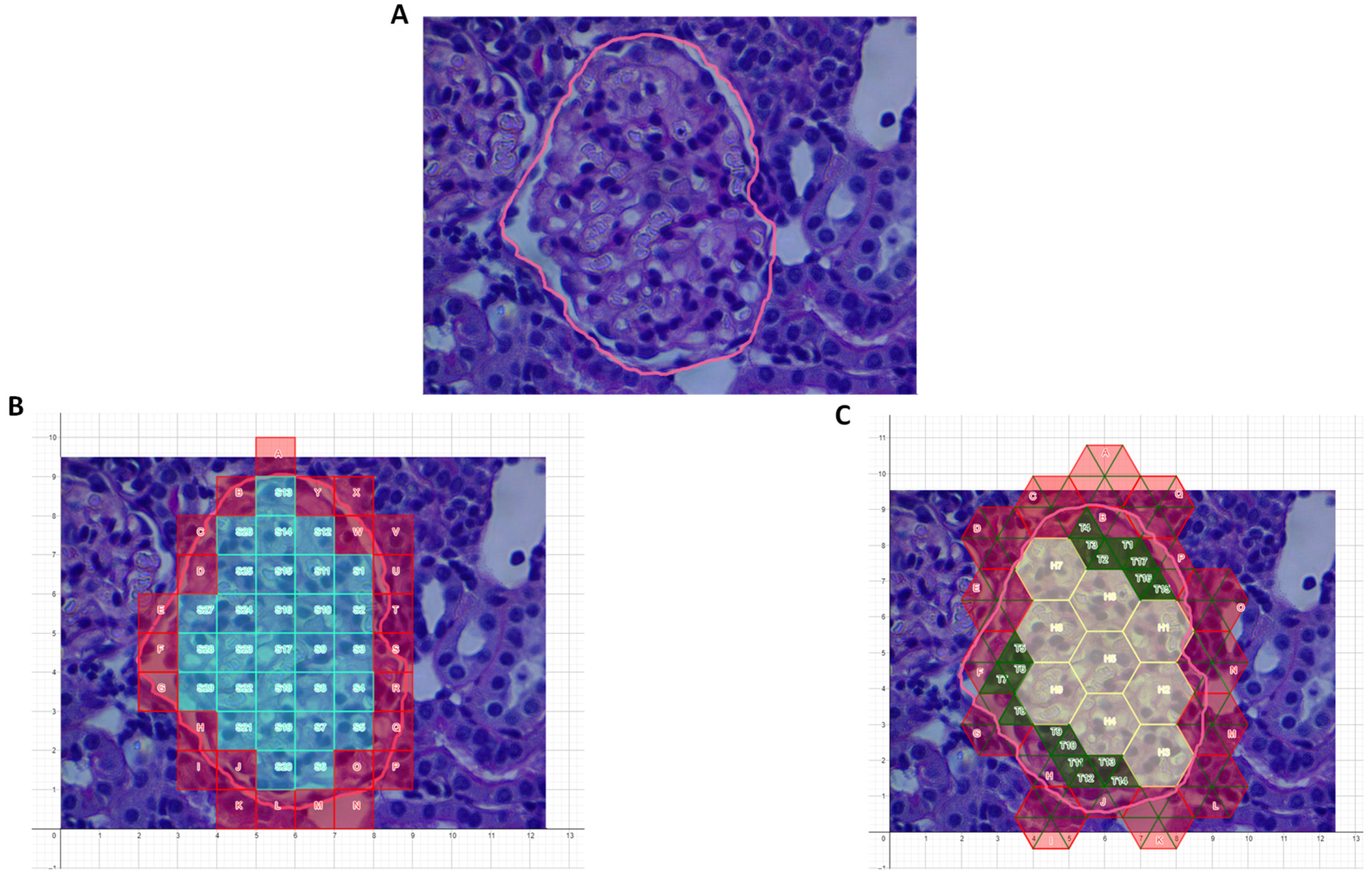
Figure 4.
Area of a renal cyst. (A) Renal cyst enclosed by a wall (region of interest lay within wall). (B) Region populated with unit squares. Only the blue/turquoise squares were completely enclosed within the region and counted. (C) Region populated with lattice comprising unit hexagons and unit triangles. Hexagons were filled in first, then triangles (green). All hexagons and green triangles lay within region of interest and were therefore counted.

Figure 5.
Refining area calculations. (A) Renal cyst enclosed by wall (region of interest lay within wall). (B) Region populated with relatively large unit squares. (C) Region populated with smaller unit squares. (D) Region populated with mixed but relatively large unit lattice. (E) Region populated with mixed but smaller unit lattice.


Table 1.
Glomerular-area determination using ImageJ, unit squares, and mixed-unit lattice.
| Glomerulus | ImageJ (unit2) | Squares (unit2) | Lattice (unit2) | Improvement (%) over Unit Squares |
|---|---|---|---|---|
| 1 | 42.5 | 29 | 31 | 7 |
| 2 | 53 | 40 | 42.4 | 6 |
| 3 | 21.3 | 15 | 15.6 | 4 |
| 4 | 29.7 | 20 | 22.5 | 13 |
Table 2.
Renal-cyst determination using ImageJ, unit squares, and mixed-unit lattice.
| Cyst | ImageJ (unit2) | Squares (unit2) | Lattice (unit2) | Improvement (%) over Unit Squares |
|---|---|---|---|---|
| 1 | 68.8 | 46 | 52.8 | 15 |
| 2 | 71.6 | 46 | 53.2 | 16 |
| 3 | 71 | 52 | 55.87 | 7 |
| 4 | 49 | 31 | 33.3 | 7 |
| 5 | 99.2 | 80 | 85.3 | 7 |
© 2019 by the author. Licensee MDPI, Basel, Switzerland. This article is an open access article distributed under the terms and conditions of the Creative Commons Attribution (CC BY) license (http://creativecommons.org/licenses/by/4.0/).
Share and Cite
MDPI and ACS Style
Narayan, R. Mixed-Unit Lattice Approach for Area Determination of Cellular and Subcellular Structures. Appl. Sci. 2019, 9, 5267. https://doi.org/10.3390/app9245267
AMA Style
Narayan R. Mixed-Unit Lattice Approach for Area Determination of Cellular and Subcellular Structures. Applied Sciences. 2019; 9(24):5267. https://doi.org/10.3390/app9245267
Chicago/Turabian StyleNarayan, Rithika. 2019. "Mixed-Unit Lattice Approach for Area Determination of Cellular and Subcellular Structures" Applied Sciences 9, no. 24: 5267. https://doi.org/10.3390/app9245267
Note that from the first issue of 2016, this journal uses article numbers instead of page numbers. See further details here.