All articles published by MDPI are made immediately available worldwide under an open access license. No special
permission is required to reuse all or part of the article published by MDPI, including figures and tables. For
articles published under an open access Creative Common CC BY license, any part of the article may be reused without
permission provided that the original article is clearly cited. For more information, please refer to
https://www.mdpi.com/openaccess.
Feature papers represent the most advanced research with significant potential for high impact in the field. A Feature
Paper should be a substantial original Article that involves several techniques or approaches, provides an outlook for
future research directions and describes possible research applications.
Feature papers are submitted upon individual invitation or recommendation by the scientific editors and must receive
positive feedback from the reviewers.
Editor’s Choice articles are based on recommendations by the scientific editors of MDPI journals from around the world.
Editors select a small number of articles recently published in the journal that they believe will be particularly
interesting to readers, or important in the respective research area. The aim is to provide a snapshot of some of the
most exciting work published in the various research areas of the journal.
Shenzhen Institutes of Advanced Technology, Chinese Academy of Sciences, Shenzhen 518055, China
2
Shenzhen College of Advanced Technology, University of Chinese Academy of Sciences, Beijing 100049, China
3
Guangdong Provincial Key Lab of Robotics and Intelligent System, Shenzhen Institutes of Advanced Technology, Chinese Academy of Sciences, Shenzhen 518055, China
4
CAS Key Laboratory of Human-Machine Intelligence-Synergy Systems, Shenzhen Institutes of Advanced Technology, Shenzhen 518055, China
*
Author to whom correspondence should be addressed.
In order to enable robots to be more intelligent and flexible, one way is to let robots learn human control strategy from demonstrations. It is a useful methodology, in contrast to traditional preprograming methods, in which robots are required to show generalizing capacity in similar scenarios. In this study, we apply learning from demonstrations on a wheeled, inverted pendulum, which realizes the balance controlling and trajectory following simultaneously. The learning model is able to map the robot position and pose to the wheel speeds, such that the robot regulated by the learned model can move in a desired trajectory and finally stop at a target position. Experiments were undertaken to validate the proposed method by testing its capacity of path following and balance guaranteeing.
After decades of development, robots have become the partners of human beings not only in the workplace, but also at home. Many efforts have been made to bring robots closer to humans. Making robots more human-like means more than making them look like humans; more importantly, it means granting them human-like behaviors. The humanoid robot seems naturally friendly because of its anthropomorphic appearance. However, the two legs of a humanoid robot might encounter many difficulties in motion because of unprecedented disturbances in complex environments. In contrast, the wheeled inverted pendulum (WIP) robot is much easier to control with fewer actuators, and would be more stable and flexible than biped robots, which makes it promising for working with humans [1,2]. Balance control and motion planning are two important issues for WIP robots. Nevertheless, to systematically solve them both is not trivial [3,4].
In various tasks undertaken by WIP robots (including mobile robot motion planning, keeping balance, and even manipulation, grasping, and human-machine cooperation with loaded robotic hands, etc.), a pre-designed controller is usually a prerequisite for robots to execute designated motions in a structured environment [5,6,7]. However, coding for simply one task is a heavy workload, not to mention that all the tasks should be addressed simultaneously by designing controllers. Furthermore, due to the fixed pattern of a manually designed controller, it is difficult for a robot to generalize to slight changes of workspace or sudden external perturbations. In this context, a methodology is desirable if it enables the robot to extract the features of the human control strategy such that it can generalize to similar tasks under the same kinds of working configurations [8].
Learning from demonstration (LfD) is one such a methodology that satisfies the above-mentioned requirements [9,10]. Specifically, LfD consists of three procedures [11], which are orderly collecting human demonstrations for the task, learning model parameters from the demonstration examples, and reproducing with the learned control model. By straightforwardly feeding the robot with demonstrations related to specific tasks, a controller implicating the human control strategy can be automatically learned, which benefits the amateur users without professional knowledge of how to design a controller. Additionally, the learned model has generalization capacity to guarantee that the robot can adapt to similar tasks, therefore avoiding the trouble of controller redesigning [12,13].
In this study, we focus on applying LfD on a wheeled inverted pendulum (Figure 1). A controller is automatically learned from demonstrations, which should be able to regulate the two-wheeled robot to move along a path similar to the demonstrated counterpart and to converge to a desired position. Additionally, the control process should be effective under both the nonholonomic constraints of two-wheeled mobile robots and the underactuated constraints that guarantee the balance of the wheeled inverted pendulum.
In order to achieve the above-mentioned control requirements, we provide a learning framework based on our previous work of learning stable and accurate dynamic system for manipulators. Different from the previous work, the proposed learning framework can handle the nonholonomic control problem of mobile robots. Meanwhile, we propose an online, state-variable estimating method that is applied during the reproduction process. The method is necessary because the nonholonomic constraints of the mobile robot and the unactuated constraints possibly deviate the robot from the expected direction. In this situation, the proposed estimating method can adjust the extra-dimensional component in the previous work appropriately according to the real robot positions, such that the trajectory accuracy can still be kept on a nonholonomic mobile robot. The contributions in this paper can be, therefore, listed as follows:
1. We provide a multi-objective learning framework to model an accurate and stable controller for a wheeled inverted pendulum, which has to take into consideration both the nonholonomic constraints of mobile robots and the underactuated constraints for balance.
2. A real-time estimating method for the extra-dimensional component (used in the reproduction process) is proposed based on a proposed constrained optimization problem, which changes the situation that the extra-dimensional component in the previous work cannot be influenced by the change of the robot positions (which is important for nonholonomic mobile robots to maintain trajectory accuracy).
The remainder of this paper is structured as follows. Section 2 introduces the related work. Section 3 formulates the problem investigated in this paper. Specific descriptions of the proposed approach are given in Section 4. Simulations and experiments are provided to validate the proposed method in Section 5. Finally, Section 6 concludes the contribution of this paper.
2. Related Work
By conventional control methodologies, the robot task is usually encoded by manually designing a controller [14,15,16]. In order to acquire more complicated control strategy from humans automatically, learning approaches are applied to yield a controller in the data-driven fashion. Spline decomposition methods [17,18] are presented to construct the robot regulators by computing the point-wise averages of the demonstrated trajectories. These methods are efficient and simple to execute, but they depend mainly on the human heuristics for trajectory synthesis.
Statistical approaches [19,20] are also prevailing for modeling robot motions. These approaches usually need a reasonable heuristic for controller programming, therefore, being possibly influenced by external perturbations. These approaches are close but still unable to generalize to similar task cases in that the choice of heuristic is decided based on specific task parameters.
The dynamic movement primitives (DMP) were proposed in [21] to effectively address the instability problem. Its main idea is to approximate a nonlinear system by several linear counterparts. In contrast to its effect on the aspect of stabilization, DMP did not emphasize on the accuracy factor when modeling complicated tasks or handling complex scenarios.
Dynamic systems (DS) based methods [22,23] were developed as a promising alternative to traditional control approaches due to its convenience, which can extract human control strategies accurately and automatically from given demonstrations. Several methods choose to model dynamic systems without considering stability constraints, which makes them possibly unstable at a target position [24,25,26]. A stable estimator of a dynamic system (SEDS) was proposed in [27] with Gaussian mixture models (GMMs) to incorporate both accuracy and stability factors. SEDS uses the Lyapunov stability condition as a constraint to optimize the parameters in the control model. It effectively captures the dynamics features from human demonstrations whilst stabilizing the robot motions. Fast and stable learning of dynamic system method (FSM-DM) in [28] handles three factors for learning a dynamic system, which includes one more factor of learning speed in addition to accuracy and stability. FSM-DM is able to teach a system fast, which is advantageous in practice when efficiency is a important requirement.
In order to reduce the influence of the accuracy against the stability dilemma, the algorithm of control-Lyapunov-function-based dynamic movements (CLF-DM) was proposed in [29]. This method is divided into three steps. First, A parameterized Lyapunov function candidate is roughly taught to be consistent with the data. Second, the control features reflected by the demonstrations are learned to guarantee the accuracy factor. Third, an online correction technique is developed to stabilize the reproduced trajectory on the fly. The neurally imprinted stable vector fields (NIVF) technique was presented as a learning framework to incorporate stable vector fields into the extreme learning machine (ELM) [30], which reproduces more accurate motions and is finally stable at the target position. The approach proposed in [31] considered using ELM network to train a Lyapunov candidate based on a specific task. The learned Lyapunov candidate is consistent with the motion trajectories related to the task; therefore, making the stability constraint based on it more slack. Accordingly, the accuracy of the learned model is also less influenced by the stability factor. -SEDS was presented in [32] to handle the trade-off of stability and accuracy by means of diffeomorphism. It transforms the original robot motions into those in a new space, where the transformed motions are consistent with a quadratic Lyapunov candidate. The method (MIMS) in [33] presented extended the SEDS scheme under the manifold immersion and submersion. Though this method can further improve the situation of stability against the accuracy dilemma, the extra-dimensional component produced by the manifold immersion is time variant. Therefore, it possibly causes performance degeneration under external perturbations.
The main feature of this paper in contrast to the previous work, is to apply learning from demonstrations on a wheeled inverted pendulum, where more robot constraints including the nonholonomic and underactuated constraints need to be taken into consideration.
3. Problem Formulation
This section formulates the problem mathematically. The path planning of a wheeled inverted pendulum can be reduced to a control problem of a wheeled robot (Figure 2), which is given as
where x and y describe the Cartesian position of the wheeled robot on its motion plane, and represents the included angle between the robot orientation and the x-axis. v represents the forward speed of the robot and represents the angular speed. The relationship between v, and , and (the speed of two wheels (Figure 2)) is as follows:
where L represents the axis width between two wheels. Meanwhile, the wheeled inverted pendulum is controlled under the underactuated constraints given as
where is the tilt angle, H is the distance between the wheel centroid and the mass, and g denotes the acceleration of gravity.
The control diagram of a robot system scheme can be seen in Figure 3. In the phase of collecting demonstrations, a motion capturer is used to collect the position and pose of the wheeled inverted pendulum at a sampling interval of . The sequence of robot positions and poses as well as the tilt angle are recorded as . In the demonstration set, n indexes the demonstrated trajectories whose total number is N. t represents the sampling instant and represents the total sampling number in the demonstration. The first-order derivatives , , , and corresponding to , , , and can be further computed as
Specially, and the demonstration have a common target position and pose; i.e., , , and . The tilt angle does not have to be zeros at last, but has to be a small number.
The demonstration generating process can be thought to result from a dynamic system as follows:
The purpose of this study was to teach a model to approximate the counterpart in Equation (5). Subsequently, we used the learned model to construct a mapping to actuate and for the nonholonomic mobile robot, which satisfies both the balance controlling and the path following requirements.
4. Learning Path Following and Balance Controlling Simultaneously
In this section, we introduce the proposed learning framework for a wheeled inverted pendulum, along with an online state-variable estimating method applied during the reproduction process.
4.1. Teaching the Control Model with the Nonholonomic and Underactuated Constraints
Instead of directly learning the controller of the wheeled inverted pendulum in the form of Equation (5), we chose to first teach the dynamic system and to subsequently transfer the learned dynamic system into a controller.
In order to let the dynamic system sufficiently capture the control features implicated in the demonstrated trajectories (i.e., the sequences of x and y), we added an extra-dimensional component z for the demonstrated trajectories based on our previous work [33], and therefore, acquired transformed trajectories denoted as . Therefore, we taught a dynamic system denoted as
where are the parameters to be learned during the learning process.
The first loss term for learning is given as Equation (7) to fit the dynamic system that generate the transformed demonstration examples .
Due to the existence of the nonholonomic constraints, we add a loss term
which is equivalent to adding mobile robot motion constraints to the learned model.
Similarly, we consider the balance control constraints by adding another loss term to be
where * denotes . Taking at an instance, is given as
The learning process is meant to decrease the weighted sum of the loss:
where are the stability constraints similar to those in [28]; and , , and denote the weighting coefficients. In this way, the learned dynamic system is hopefully accurate and stable under the nonholonomic constraints and underactuated constraints like those shown in Figure 2.
When reproducing the learned dynamic system, we acquire the prediction of the forward velocity and the angular velocity by
Based on Equation (2), we can acquire the predicted wheel velocities and .
4.2. Estimating the Extra-Dimensional Component by a Constrained Optimization Related to the Learned Dynamic System
In spite of the fact that we have incorporated the loss terms and for the learning process to handle the nonholonomic constraints and the underactuated constraints, the controller (Equations (12) and (13)) yielded by the learned dynamic system still possibly fails to regulate to expected x and y at some instances due to these two constraints. The extra-dimensional component z cannot be influenced by the deviations of x and y; therefore, the accumulation effect might reduce the accuracy. This section introduces an online state variable estimating method to overcome this situation.
When reproducing the learned dynamic system, the extra-dimensional component of the initial input for the learned dynamic system is computed by a constant ratio as in the following
where is determined by
The rule in Equation (15) to decide the constant ratio comes from a natural thought shown in Figure 4.
The proposed estimating approach is mainly based on a constrained optimization problem related to the learned dynamic system. The general idea can be seen in Figure 5. Specifically, the learned dynamic system predicts the state variable with the state variable as model input.
Suppose that the robot’s actual state variable is actually under the robot constraints and the external perturbations (with only predicted unchanged because it is a virtual component and cannot be influenced by any external factors).
In order to find an appropriate value to adjust the extra-dimensional component , we suppose the actual state variable is a direct output of the learned dynamic sub-system,
without the influences of the external factors (Figure 5). Additionally, we fixed the values of and ; i.e., considering them as constants at that instant. Therefore, the corresponding input of the sub-system satisfying that
where is the sampling instant during the reproduction process.
Meanwhile, is supposed to be near ; accordingly, the derivative directions at these two points are expected to be close as well, which constitutes an optimization constraint as
where is a small positive number.
The assumed sub-system input in the instant is subsequently acquired by solving the following constrained optimization problem with as the initial guess.
Finally, we use the optimized as input to the learned sub-system , outputting
Replacing by , we can acquire the adjusted extra-dimensional component at the instant.
5. Experiment
In this section, we validate the proposed method on a real wheeled inverted pendulum with a motion capturer to observe the position and pose information (as shown in Figure 6). The wheeled inverted pendulum uses STM32 single chip computer as the processor to control the velocities of its two wheels. The Bluetooth interface was provided for communications between the STM32 single chip computer and the upper computer. We used the Vicon Tracker 3.4 motion capturer to observe the state of the wheeled inverted pendulum in real-time. The motion capturer can send the observed state to the local network that it is connected to. We, therefore, built software to receive the state observed from the motion capturer. After handling the date received through the algorithm in the upper computer, we subsequently send orders to the STM32 computer to actuate the wheeled inverted pendulum at an interval of 0.005 s.
The effectiveness of the proposed algorithm was verified by applying it to the path following task. We collected three kinds of trajectories with three groups of demonstrations for each kind (Figure 7). The recorded demonstrated trajectories were used to train the dynamic system in Equation (6). The sampling interval was also set as 0.005 s.
Subsequently, we picked a demonstration from each kind of trajectory as the reference trajectory. We let the robot start from a different position to follow the reference trajectory.
The results by the proposed method and two traditional control methods [34,35] are shown in Figure 8. It can be seen that the proposed learning method can smoothly follow the reference trajectory and finally converge to the target position.
We also used the swept error area standard (SEA) [29] to evaluate the proposed method and the traditional methods [34,35] quantitatively. The SEA standard measures the difference between the generated and the reference trajectories by their included area (Figure 9). The meaning of the SEA standard can be simply thought as a fact that the generated trajectory should be enough close to the reference counterpart, if the evaluated controller is effective in path following. The computing formula is given by
where and are sampling points, respectively, from the generated and reference trajectories. is the area of the tetragon enclosed by the four adjacent points along the trajectories.
The SEA results by the proposed method and the approaches in [34,35] can be seen in Table 1. From the results, we can see that the proposed method can better achieve the capacity of path following; i.e., the error between the generated trajectory by the learned controller and the reference trajectory is smaller.
6. Conclusions
This study investigated applying learning from demonstrations on a wheeled inverted pendulum. We took into consideration four aspects: the control under nonholonomic constraints, keeping the pendulum balanced, stability, and accuracy. We incorporated the nonholonomic and underactuated constraints into the learned dynamic system by adding corresponding loss terms for optimizing. Additionally, we proposed an online, state variable estimating method to adjust the extra-dimensional component in the reproduction period such that the accuracy can be further improved even under the robot constraints, including the nonholonomic and underactuated constraints. In future work, we plan to exploit deeper control features in demonstrations, and improve the controller more intelligently by adding more human-like constraints during the learning process.
Author Contributions
Conceptualization, S.J. and Y.O.; Methodology, S.J. and Y.O.; Software, S.J.; Validation, Y.O.; formal analysis, S.J.; Investigation, Y.O.; Resources, Y.O.; data curation, S.J.; Writing—original draft preparation, S.J.; Writing—review and editing, Y.O.; Visualization, S.J.; Supervision, Y.O.; project administration, Y.O.; funding acquisition, Y.O.
Funding
This work was jointly supported by National Natural Science Foundation of China (Grant No. U1613210), Guangdong Special Support Program (2017TX04X265), Science and Technology Planning Project of Guangdong Province (2019B090915002), and Shenzhen Fundamental Research Program (JCYJ20170413165528221).
Conflicts of Interest
The authors declare no conflict of interest.
References
Takahashi, S.; Nonoshita, H.; Takahashi, Y.; Maeda, Y.; Nakamura, T. Inverted-pendulum mobile robot motion learning from human player observation. In SCIS & ISIS SCIS & ISIS 2010; Japan Society for Fuzzy Theory and Intelligent Informatics: Okayama, Japan, 2010; pp. 211–216. [Google Scholar]
Lee, G.H.; Jung, S. Line tracking control of a two-wheeled mobile robot using visual feedback. Int. J. Adv. Robot. Syst.2013, 10, 177. [Google Scholar] [CrossRef] [Green Version]
Villacres, J.; Viscaino, M.; Herrera, M.; Camacho, O.; Chavez, D. Two-wheeled inverted pendulum path planning: An experimental validation. In Proceedings of the IEEE Ecuador Technical Chapters Meeting (ETCM), Guayaquil, Ecuador, 12–14 October 2016; pp. 1–6. [Google Scholar]
Kim, S.; Kwon, S.J. Nonlinear optimal control design for underactuated two-wheeled inverted pendulum mobile platform. IEEE/ASME Trans. Mechatron.2017, 22, 2803–2808. [Google Scholar] [CrossRef]
Xu, C.; Ou, Y.; Schuster, E. Sequential linear quadratic control of bilinear parabolic PDEs based on POD model reduction. Automatica2011, 47, 418–426. [Google Scholar] [CrossRef]
Xu, C.; Ou, Y.; Dalessio, J.N.; Schuster, E.; Luce, T.C.; Ferron, J.R.; Walker, M.L.; Humphreys, D.A. Ramp-up current profile control of tokamak plasmas: A numerical optimization approach. IEEE Trans. Plasma Sci.2010, 38, 163–173. [Google Scholar] [CrossRef]
Xu, C.; Schuster, E.; Vazquez, R.; Krstic, M. Stabilization of linearized 2D magnetohydrodynamic channel flow by backstepping boundary control. Syst. Control Lett.2008, 57, 805–812. [Google Scholar] [CrossRef]
Argall, B.D.; Chernova, S.; Veloso, M.; Browning, B. A survey of robot learning from demonstration. Robot. Autonomous Syst.2009, 57, 469–483. [Google Scholar] [CrossRef]
Pignat, E.; Calinon, S. Learning adaptive dressing assistance from human demonstration. Robot. Auton. Syst.2017, 93, 61–75. [Google Scholar] [CrossRef] [Green Version]
Luo, J.; Yang, C.; Su, H.; Liu, C. Learning Generalization, and Obstacle Avoidance with Dynamic Movement Primitives and Dynamic Potential Fields. Appl. Sci.2019, 9, 1535. [Google Scholar] [CrossRef] [Green Version]
Billard, A.G.; Calinon, S.; Dillmann, R. Learning from Humans. In Springer Handbook of Robotics, 2nd ed.; Springer: Midtown Manhattan, NY, USA, 2016; pp. 1995–2014. [Google Scholar]
Moridian, B.; Kamal, A.; Mahmoudian, N. Learning Navigation Tasks from Demonstration for Semi-Autonomous Remote Operation of Mobile Robots. In Proceedings of the 2018 IEEE International Symposium on Safety, Security, and Rescue Robotics (SSRR), Philadelphia, PA, USA, 6–8 August 2018. [Google Scholar]
Mbanisi, K.C.; Kimpara, H.; Meier, T.; Gennert, M.; Li, Z. Learning Coordinated Vehicle Maneuver Motion Primitives from Human Demonstration. In Proceedings of the 2018 IEEE International Symposium on Safety, Security, and Rescue Robotics (SSRR), Philadelphia, PA, USA, 6–8 August 2018. [Google Scholar]
Wang, H.; Liu, Y.H. Uncalibrated visual tracking control without visual velocity. IEEE Trans. Control Syst. Technol.2010, 18, 1359–1370. [Google Scholar] [CrossRef]
Wang, H.; Liu, Y.H. A New Approach to Dynamic Eye-in-hand Visual Tracking Using Nonlinear Observers. Ifac Proc. Vol.2009, 42, 711–716. [Google Scholar] [CrossRef]
Wang, H.; Chen, W.; Yu, X.; Deng, T.; Wang, X.; Pfeifer, R. Visual servo control of cable-driven soft robotic manipulator. In Proceedings of the 2013 IEEE/RSJ International Conference on Intelligent Robots and Systems, Tokyo, Japan, 3–7 November 2013. [Google Scholar]
Hwang, J.H.; Arkin, R.C.; Kwon, D.S. Mobile robots at your fingertip: Bezier curve on-line trajectory generation for supervisory control. In Proceedings of the 2003 IEEE/RSJ International Conference on Intelligent Robots and Systems, Las Vegas, NV, USA, 27–31 October 2003. [Google Scholar]
Aleotti, J.; Caselli, S. Robust trajectory learning and approximation for robot programming by demonstration. Robot. Autonomous Syst.2006, 54, 409–413. [Google Scholar] [CrossRef]
Kulic, D.; Takano, W.; Nakamura, Y. Incremental Learning, Clustering and Hierarchy Formation of Whole Body Motion Patterns using Adaptive Hidden Markov Chains. Int. J. Robot. Res.2008, 27, 761–784. [Google Scholar] [CrossRef]
Muhlig, M.; Gienger, M.; Hellbach, S.; Steil, J.J.; Goerick, C. Task-level imitation learning using variance-based movement optimization. In Proceedings of the IEEE International Conference on Robotics and Automation, Kobe, Japan, 12–17 May 2009; pp. 1177–1184. [Google Scholar]
Pastor, P.; Hoffmann, H.; Asfour, T.; Schaal, S. Learning and Generalization of Motor Skills by Learning from Demonstration. In Proceedings of the IEEE International Conference on Robotics and Automation, Kobe, Japan, 12–17 May 2009. [Google Scholar]
Khansari-Zadeh, S.M.; Billard, A. Imitation learning of globally stable non-linear point-to-point robot motions using nonlinear programming. In Proceedings of the IEEE/RSJ 2010 International Conference on Intelligent Robots and Systems, Taipei, Taiwan, 18–22 October 2010. [Google Scholar]
Hersch, M.; Guenter, F.; Calinon, S.; Billard, A. Dynamical system modulation for robot learning via kinesthetic demonstrations. IEEE Trans. Robot.2008, 24, 1463–1467. [Google Scholar] [CrossRef] [Green Version]
Rasmussen, C.E. Gaussian processes for machine learning. Int. J. Neural Syst.2006, 14, 69–106. [Google Scholar]
Schaal, S.; Atkeson, C.G.; Vijayakumar, S. Scalable techniques from nonparametric statistics for real time robot learning. Appl. Intell.2002, 17, 49–60. [Google Scholar] [CrossRef]
Dempster, A.P.; Laird, N.M.; Rubin, D.B. Maximum Likelihood from Incomplete Data via the EM Algorithm. J. R. Stat. Soc. B1977, 39, 1–38. [Google Scholar]
Khansari-Zadeh, S.M.; Billard, A. Learning stable nonlinear dynamical systems with Gaussian mixture models. IEEE Trans. Robot.2011, 27, 943–957. [Google Scholar] [CrossRef] [Green Version]
Duan, J.; Ou, Y.; Hu, J.; Wang, Z.; Jin, S.; Xu, C. Fast and Stable Learning of Dynamical Systems Based on Extreme Learning Machine. IEEE Trans. Syst. Man Cybern. Syst.2017, 49, 1–11. [Google Scholar] [CrossRef]
Khansari-Zadeh, S.M.; Billard, A. Learning control Lyapunov function to ensure stability of dynamical system-based robot reaching motions. Robot. Autonomous Syst.2014, 62, 752–765. [Google Scholar] [CrossRef] [Green Version]
Lemme, A.; Neumann, K.; Reinhart, R.F.; Steil, J.J. Neurally imprinted stable vector fields. In Proceedings of the European Symposium on Artificial Neural Networks, Bruges, Belgium, 24–26 April 2013; pp. 327–332. [Google Scholar]
Neumann, K.; Lemme, A.; Steil, J.J. Neural learning of stable dynamical systems based on data-driven Lyapunov candidates. In Proceedings of the IEEE International Conference on Intelligent Robots and Systems, Tokyo, Japan, 3–7 November 2013; pp. 1216–1222. [Google Scholar]
Neumann, K.; Steil, J.J. Learning robot motions with stable dynamical systems under diffeomorphic transformations. Robot. Autonomous Syst.2015, 70, 1–15. [Google Scholar] [CrossRef] [Green Version]
Jin, S.; Wang, Z.; Ou, Y.; Feng, W. Learning Accurate and Stable Dynamical System Under Manifold Immersion and Submersion. In IEEE Transactions on Neural Networks and Learning Systems; The Institute of Electrical and Electronics Engineers (IEEE): Piscataway, NJ, USA, 2019. [Google Scholar]
Xia, D.; Yao, Y.; Cheng, L. Indoor Autonomous Control of a Two-Wheeled Inverted Pendulum Vehicle Using Ultra Wide Band Technology. Sensors2017, 17, 1401. [Google Scholar] [CrossRef] [PubMed]
Zhou, Y.; Wang, Z.; Chuang, K. Turning Motion Control Design of a Two-Wheeled Inverted Pendulum Using Curvature Tracking and Optimal Control Theory. J. Optim. Theory Appl.2019, 181, 634–652. [Google Scholar] [CrossRef] [Green Version]
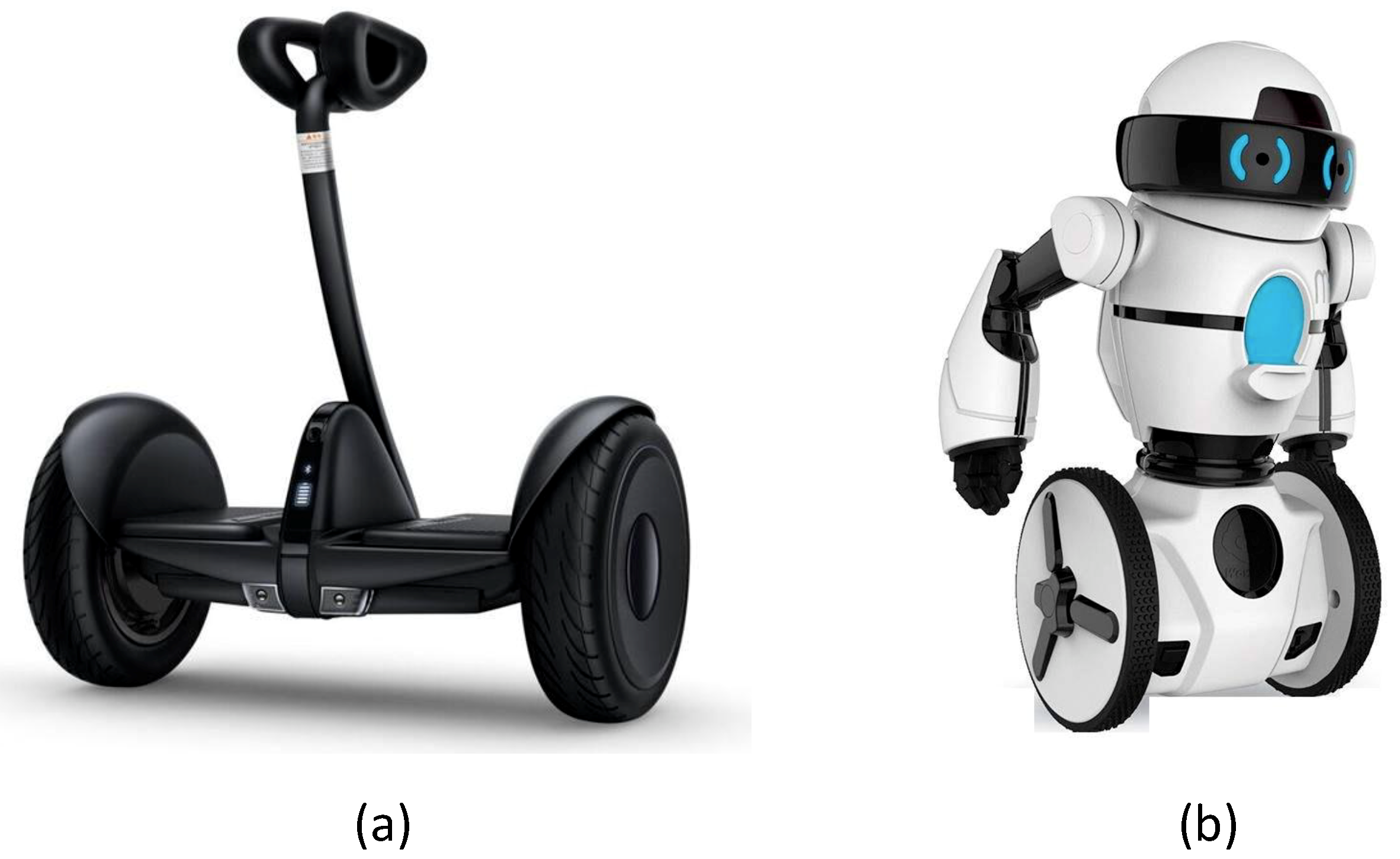
Figure 1.
The applications of a wheeled inverted pendulum. (a) shows a manned balanced vehicle; (b) shows a serving robot on a two-wheeled self-balancing platform.
Figure 1.
The applications of a wheeled inverted pendulum. (a) shows a manned balanced vehicle; (b) shows a serving robot on a two-wheeled self-balancing platform.
Figure 2.
The control constraints of a wheeled inverted pendulum.
Figure 2.
The control constraints of a wheeled inverted pendulum.
Figure 3.
The control scheme of learning from demonstrations for a wheeled inverted pendulum.
Figure 3.
The control scheme of learning from demonstrations for a wheeled inverted pendulum.
Figure 4.
An intuitive thought to decide the extra-dimensional component for the initial input. In (a), if the start points are equally distant from the target point, their corresponding extra-dimensional components are supposed to be closed to equal as well; i.e., provided that ; in (b), if the distances of two start points from the target point are not equal, we suppose that the ratio of their extra-dimensional components approximates that of their distances to the target points; i.e., .
Figure 5.
Adjusting the extra-dimensional component by a constructed constrained optimization problem. In (a), the learned dynamic system outputs the predicted robot position and the corresponding extra-dimensional component at instant (with the state variable at the instant as system input). The external factors, including the nonholonomic constraints and underactuated constraints, influence the robot’s movement, and the robot moves to an actual position deviating from the predicted one. In order to adjust the extra-dimensional component which cannot be influenced by the external factors, we suppose there is a similar robot motion trajectory (red curve on the x-y plane in (b)) passing near the current robot trajectory (blue curve on the x-y plane in (b)). The robot motion trajectory passes through actual robot position at the instant, which is also yielded by the learned dynamic system while it starts from another start point. In (c), considering the two trajectories (red and blue curves in the x-y-z Cartesian space) are alike, the derivative directions at the reproduced points on them at the instant should be also similar. Using those as constraints and combining the learned dynamic system function, the previous point on the red marked trajectory at instant can be acquired by solving the constrained optimization in Equation (19). Inputting it to the learned dynamic system, the next state variable can be predicted, the extra-dimensional component of which is the value to be used for adjusting the current component at instant.
Figure 6.
The configuration of the experiment. (a) A wheeled inverted pendulum with markers attached on it; (b) a laptop as the upper computer sends orders to the wheeled inverted pendulum through Bluetooth; (c) the hardware of the motion capturer. There are four cameras to observe the position and pose information of the wheeled robot in total; (d) shows the software interface of the motion capturer. It can send the position and pose information through UDP protocol such that the upper computer can receive the information in real-time.
Figure 7.
The demonstrations given by humans to teach a model that can regulate a wheeled inverted pendulum to undertake path following task.
Figure 7.
The demonstrations given by humans to teach a model that can regulate a wheeled inverted pendulum to undertake path following task.
Figure 8.
The results by the proposed method and the methods in [34,35]. The upper row shows the general trajectory shape of the path following. The lower row records the path following results through MATLAB.
Figure 8.
The results by the proposed method and the methods in [34,35]. The upper row shows the general trajectory shape of the path following. The lower row records the path following results through MATLAB.
Figure 9.
Illustrative example of swept error area standard (SEA) computing functional. The tetragon area enclosed by points and in the generated trajectory, and points and in the reference trajectory represent the error between the two sampling points of the generated trajectory and the counterparts of the reference trajectory. The sum of all such tetragon areas are, therefore, used to measure the error between the generated and reference trajectories.
Jin, S.; Ou, Y.
A Wheeled Inverted Pendulum Learning Stable and Accurate Control from Demonstrations. Appl. Sci.2019, 9, 5279.
https://doi.org/10.3390/app9245279
AMA Style
Jin S, Ou Y.
A Wheeled Inverted Pendulum Learning Stable and Accurate Control from Demonstrations. Applied Sciences. 2019; 9(24):5279.
https://doi.org/10.3390/app9245279
Chicago/Turabian Style
Jin, Shaokun, and Yongsheng Ou.
2019. "A Wheeled Inverted Pendulum Learning Stable and Accurate Control from Demonstrations" Applied Sciences 9, no. 24: 5279.
https://doi.org/10.3390/app9245279
Note that from the first issue of 2016, this journal uses article numbers instead of page numbers. See further details here.
Article Metrics
No
No
Article Access Statistics
For more information on the journal statistics, click here.
Multiple requests from the same IP address are counted as one view.
Jin, S.; Ou, Y.
A Wheeled Inverted Pendulum Learning Stable and Accurate Control from Demonstrations. Appl. Sci.2019, 9, 5279.
https://doi.org/10.3390/app9245279
AMA Style
Jin S, Ou Y.
A Wheeled Inverted Pendulum Learning Stable and Accurate Control from Demonstrations. Applied Sciences. 2019; 9(24):5279.
https://doi.org/10.3390/app9245279
Chicago/Turabian Style
Jin, Shaokun, and Yongsheng Ou.
2019. "A Wheeled Inverted Pendulum Learning Stable and Accurate Control from Demonstrations" Applied Sciences 9, no. 24: 5279.
https://doi.org/10.3390/app9245279
Note that from the first issue of 2016, this journal uses article numbers instead of page numbers. See further details here.


