Feature Deep Continuous Aggregation for 3D Vehicle Detection

Abstract

3D object detection has recently become a research hotspot in the field of autonomous driving. Although great progress has been made, it still needs to be further improved. Therefore, this paper presents FDCA, a feature deep continuous aggregation network using multi-sensors for 3D vehicle detection. The proposed network adopts a two-stage structure with the bird’s-eye view (BEV) map and the RGB image as an input. In the first stage, two feature extractors were used to generate feature maps with the high-resolution and representational ability for each input view. These feature maps were then fused and fed to a 3D proposal generator to obtain the reliable 3D vehicle proposals. In the second stage, the refinement network aggregated the features of the proposal regions further and performed classifications, a 3D bounding boxes regression, and orientation estimations to predict the location and heading of vehicles in 3D space. The FDCA network proposed was trained and evaluated on the KITTI 3D object detection benchmark. The experimental results of the validation set illustrated that compared with other fusion-based methods, the 3D average precision (AP) could achieve 76.82% on a moderate setting while having real-time capability, which was higher than that of the second-best performing method by 2.38%. Meanwhile, the results of ablation experiments show that the convergence rate of FDCA was much faster and the stability was also much better, making it a candidate for application in autonomous driving.

1. Introduction

In an autonomous driving system, 3D vehicle detection is essential to ensure safety, which can provide the reliable relative location and speed information between the vehicle and other traffic participants for drivers or an intelligent control system to avoid collisions. Unlike classical 2D object detection methods [1,2] that obtain objects’ categories and bounding boxes in the image plane, 3D object detection methods can reveal more detailed information about the objects, including the physical size, relative position, and heading information. This information is crucial for intelligent driving tasks, such as behavior decision, path planning, navigation control, collision avoidance, etc. However, even with this information, a lower performance is achieved compared with that of 2D object methods. On the KITTI dataset, the average precision (AP) of 2D vehicle detectors is about 15% higher than that of 3D detectors [3]. Therefore, 3D object detection methods need to be further studied.

According to the sensors most commonly used in the traffic scene, 3D object detection methods can be roughly divided into three categories [4]: image-based, point-cloud-based, and fusion-based methods. Image data can provide abundant texture properties, which are of great significance to object recognition. However, the lack of explicit depth information restricts the accuracy of position and bounding box regression for objects, especially long-range small-scale objects. Point cloud data can retain the physical size and depth information of the object, which is beneficial to position and 3D bounding box regression. However, due to its sparsity and lack of texture information, many kinds of objects have similar feature representations in 3D point cloud space, which is not conducive to object recognition. Fusion-based methods can make full use of the advantages of the two sensors and achieve a better detection performance.

Influenced by the rapid development of 2D object detection methods, a LiDAR(Light Detection and Ranging)point cloud is usually projected as pseudo images, such as a FV (front view) map [5] or a bird’s-eye view (BEV) map [6,7,8], and then the pseudo images and RGB images are fed to the two-stage 2D detector with an extension to perform 3D bounding box regression, classification, and orientation estimation.

The fusion-based methods have achieved good performance, but there are still some shortcomings to be solved. First, projecting the LiDAR point cloud as a BEV map creates a loss of a large amount of information, especially the height information, causing a significant gap between AP_BEV and AP_3D. With the KITTI dataset, the AP_BEV is more than 10% higher than AP_3D. Being able to retain as much information as possible on the BEV map will directly affect the final detection results. Second, the procedure of the two-stage detection structure is complex, the utilization efficiency of feature is low, and the parameters are redundant, causing a low generalization capability of the network. For example, the backbone network usually uses a VGG16-like [9] (visual geometry group) structure in the feature extractor; the refinement network adopts cascaded, fully connected layers (FC) [6,7], which lead to a huge number of parameters and a lower performance compared with other methods. A standard VGG16 network has more than 138 million parameters; some literature has proved that most of them have little effect on the final results [10,11]. ResNet [10] introduces a residual structure with only 25.5 million parameters, but the classification performance is higher than that of VGG16 with the ImageNet dataset. Deep Compression [11] achieves about 40 times the compression rate based on VGG16 networks by pruning, trained quantization, and Huffman coding, and the performance of the network has risen rather than fallen. In addition, the design of a loss function for 3D object detection is more complex than that of 2D object detection. Apart from classification and bounding box regression, the output target of the 3D object detection method has one more orientation estimation; meanwhile, there is also one more dimension in the bounding box regression. The diversity of loss categories and calculation methods makes it difficult to optimize the network. Being able to balance the loss weight of each optimization target is equally important to the final detection results.

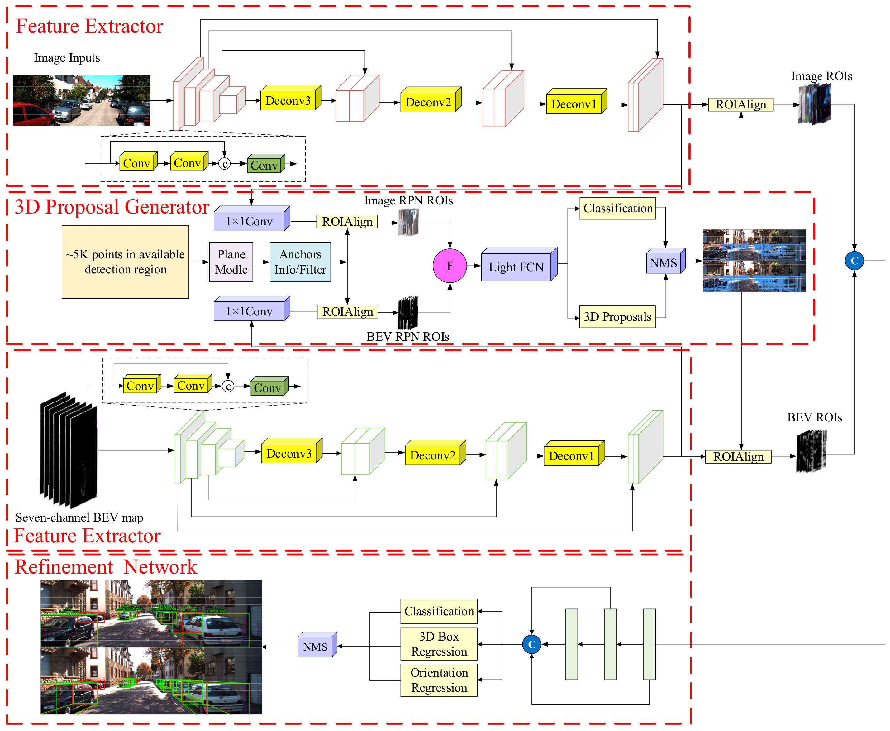
In this paper, a feature deep continuous aggregation (FDCA) network is proposed to solve the above problems (Figure 1). The contributions of this work are as follows:

• A seven-channel BEV map was generated, which contains one global height channel, five local height channels, and one density channel to preserve the local and global features. The five local height channels preserve the local location correlation among layers by global normalization.
• The feature deep continuous aggregation (FDCA) architecture is proposed to improve the generalization ability of the network. The abstract features were fused continuously and deeply by concatenating different feature layers in the feature extractors and the refinement network.
• RoIAlign was exploited to improve the cropping accuracy of features for proposal regions.
• A light fully convolutional network (FCN) was adopted to reduce the computation load and memory requirements in the 3D proposal generator.
• A loss category weight mask was used to balance the proportions of different loss categories in the total loss, and two refined regression loss weight masks were exploited to improve the regression accuracy in high dimensions.

The structure of this paper is as follows. The related works are introduced in Section 2. The proposed network of this paper is illustrated in Section 3. The results of comparison experiments and ablation experiments are discussed in Section 4. Finally, the conclusions are given in Section 5.

2. Related Works

In this section, we briefly review existing works on 3D object detection methods according to the following three categories: image-based, point-cloud-based, and fusion-based methods.

2.1. Image-Based Methods

Image-based methods usually perform 2D detection on the image plane and then the detection results are extrapolated to 3D space through reprojection constraints or bounding boxes regression.

Xiang et al. [12] generated 3D voxel patterns (3DVP) representation through aligning the 3D CAD (computer aided design) model with the image, then performed a 2D detection and projected the results to 3D space to obtain a pose estimation. 3D object proposals (3DOP) [13] exploits stereo imagery to recover depth information and minimizes an energy function to generate 3D box proposals; then, these reliable proposals are classified using a region convolutional neural networks (R-CNN) network. Mono3D [14] shares the same pipeline as 3DOP, which generates 3D proposals from a monocular image. The proposals are passed to a Fast R-CNN [15] network to perform classification and a 3D bounding boxes regression. Zia and coworkers [16,17] introduced a detailed geometry representation that uses more than just 3D bounding boxes, which can obtain the pose estimation of the object and 3D wireframes with relative positions of object parts on the image plane. Deep MANTA (many-task network) [18] first obtains the 2D bounding box regression and the parts localization using a two-stage refined region proposal network (RPN) on an RGB image. Then, the detection results are matched with the prior 3D model to obtain the 3D pose.

2.2. Point-Cloud-Based Methods

From the existing works, point-cloud-based methods can be refined into three subcategories: projection-based, voxel representation, and raw point cloud methods.

2.2.1. Projection-Based

Projection-based methods usually project a raw point cloud into pseudo images, then detect objects using a 2D detection framework with an extension to regress 3D bounding boxes.

VeloFCN [5] projects raw point cloud data onto a 2D FV map and directly performs classification and 3D bounding box regression using a fully convolutional network. Yu et al. [19] generated a 3-channel BEV map representation through projecting a 3D point cloud and exploited the Faster R-CNN architecture to output 3D bounding boxes with orientation information. Complex-YOLO (you only look once) [20] converts the 3D point cloud to overlooking perspectives to generate a RGB-map, which is encoded by height, intensity, and density information, then performs a network that expands YOLOv2 [2] by a specific complex regression strategy to output the 3D bounding box regression and orientation estimation of the object. BirdNet [8] proposes a novel encoding that normalizes the density channel to generate the BEV map. The Faster R-CNN structure is then used to perform the 3D bounding box regression and orientation estimation. PIXOR (ORiented 3D object detection from PIXel-wise neural network predictions) [21] converts the point cloud into a BEV map, where the value of each cell is encoded as an occupancy rather than a height. Then, features are extracted by a ResNet network and passed to a classification head and a regression head to obtain the detection results.

2.2.2. Voxel Representations

Voxel representation methods usually divide the raw point cloud into several voxels according to a certain size. Some methods perform a 3D convolution operation to detect objects directly in 3D space, while other methods extract features from each voxel to form a pseudo image, and then use a 2D convolution backbone and a 3D detection head to output the detection results.

In 3D fully convolutional network (3DFCN) [22], the point clouds are represented as a binary volumetric, which is fed to a 3D fully convolutional network to predict the 3D bounding boxes and the orientation estimation of the vehicles. The expensive 3D convolution operation limits the real-time performance. Vote3Deep [23] divides the point cloud into 3D grids; then, the 3D sliding window method is used to determine whether each window contains vehicles or not. In order to reduce the model’s complexity, sparse convolution layers are used to avoid many empty convolution operations. Sparsely embedded convolutional detection (SECOND) [24] also divides the point clouds into grids and improves the sparse convolution method, which can greatly increase the real-time performance. Pointpillars [25] proposes a novel encoding method that exploits PointNet [26] to learn the feature vector from each vertical pillar; then, these feature vectors are treated as pseudo images, which are fed to a 2D convolution backbone and detection head to perform 3D detection.

2.2.3. Raw Point Cloud Methods

In order to avoid information loss, this kind of method directly takes the raw point cloud as the input to predict the 3D bounding box regression and the orientation estimation of the object.

PointNet [26] is a pioneering deep neural network that directly processes disordered point cloud data. It applies an input transformation and a feature transformation to extract features from each point, then aggregates the point features by max-pooling to output the classification scores for k classes. However, PointNet lacks the extraction and processing of local features, which limits its abilities of recognition and generalization in complex scenes. PointNet++ [27] exploits the hierarchical structure to extract local features for the better recognition of fine-grained patterns. In addition, density adaptation is added to the network to process point cloud data more accurately and reasonably. VoxelNet [28] is designed with a novel voxel feature coding (VFE) mode, where the network can learn complex features to describe local 3D shape information by stacking multiple VFE layers. Then, 3D convolution further aggregates the local voxel features, which are finally fed to an RPN to output the detection results. The core framework of Voxel-FPN [29] includes the encoder network and the corresponding decoder. The encoder extracts multi-scale voxel information in a bottom-up manner, while the decoder fuses multiple feature maps from different scales in a top-down manner. Then, an RPN network is utilized to output the detection results.

2.3. Fusion-Based Methods

Fusion-based methods fuse both the images and point cloud, which allow modalities to interact and complement each other. Architectures usually rely on the RPN to generate reliable proposals from each feature view. The corresponding features are further fused according to three types [6]: early fusion, late fusion, and deep fusion.

Multi-View 3D network (MV3D) [6] and aggregate view object detection (AVOD) [7] take the point cloud and RGB image as the network’s input, where the abstract and high-resolution features generated by feature extractors are fused and passed to a 3D RPN to generate proposals. The corresponding features from each branch are further fused to predict categories and 3D bounding boxes. The network of MV3D [6] consists of three input branches: BEV, FV, and RGB images. 3D RPN is used to generate proposals on the BEV feature map only, where corresponding features of each proposal are then aggregated in a deep fusion scheme. Compared to MV3D, the input representations of AVOD [7] are only the BEV maps and RGB images. The feature extractor adopts feature pyramid networks (FPN) [30] to generate a high-resolution feature map. Meanwhile, the 3D proposals are generated based on both the BEV and image feature maps. An early fusion scheme is introduced to output the classification and refined 3D bounding boxes for each proposal.

Different from the above two methods, the method of Du et al. [31] performs 2D detection on a RGB image to generate the 2D bounding boxes, which are then projected to a 3D point cloud space to select the corresponding set of points. With this set, a model-fitting algorithm is introduced to generate the 3D bounding box of the vehicles. Subsequently, a CNN network is proposed to refine the detected 3D bounding boxes. Frustum Point-Net [32] uses a 2D detector to generate proposals in the image plane, then extrapolates these proposals to a 3D point cloud space, resulting in frustums region proposals. 3D instance segmentation is performed for the obtained frustums region proposals using PointNet++; then, a T-net is used to perform the classification and 3D bounding boxes regression.

3. Approach

The proposed network consists of three parts: two feature extractors, a 3D proposal generator, and a refinement network, the detailed network structure is shown in Figure 1. Feature extractors were used to generate high-resolution feature maps from both the BEV map and RGB image. Both feature maps were then fused to generate non-oriented region proposals using a 3D proposal generator. Finally, the corresponding features from each proposal were fed to the refinement network for the 3D bounding box regression, orientation estimation, and classification.

3.1. Seven-Channel BEV Map

Considering the disorder and sparsity of a point cloud, it cannot be directly processed by 2D convolution layers. Therefore, References [6,7,8,19,20,21] project the raw point cloud as a BEV map to output the detection results using a 2D detector. In this paper, a seven-channel BEV map was generated, which contained five local height channels, one global height channel, and one density channel.

There were about 120 K points in each frame of the point cloud, which is large and only some of them were in the area of the image plane. Therefore, the point cloud was first cropped to give a fixed region to ensure that the reserved points (about 20 K) were included in the field of view of the camera. Then, the reserved points were divided into m × n × k voxel grids with a 0.1-m resolution.

Along the Z-axis, k voxel grid layers were divided into five equal slices to generate local height channels encoded with the maximum height in each voxel grid. To avoid destroying the local correlated between layers, every equal slice was globally normalized:

$$BE{V}_l^i=\frac{P_i\left(h_{max}\right)}{P\left(H\right)},$$

(1)

where $BE{V}_l^i$ represents the ith local height channel of the BEV map, $P_i\left(h_{max}\right)$ is the maximum height of points in the ith slice, and $P\left(H\right)$ is the height of all selected point clouds.

In References [6,7], the global height feature of the point cloud was not considered. To solve this problem, a global height representation was generated and added into the BEV map as the sixth channel:

$$BE{V}_g=\frac{P\left(h_{max}\right)}{P\left(H\right)},$$

(2)

where P(h_max) is the maximum height of points in each height pillar.

The seventh BEV channel was a density channel that followed the procedure described in Ku et al. [7]. The seven-channel BEV map is shown in Figure 2.

3.2. Feature Deep Continuous Aggregation Network

3.2.1. The Feature Extractor

For the feature extractor, the FPN structure is often used as the backbone network. FPN is an excellent network that not only has a high resolution, but also has abstract representation capability. Many methods [7,29,30] have proved that FPN is a general network, and the performance of a network with FPN is much better than that without FPN. Therefore, FPN architecture was adopted as the backbone network in this paper.

The full-resolution FPN network includes an encoder and a decoder, as shown in Figure 3. The structure of encoder is usually VGG16-like, which is used to generate abstract complex features, while a bottom-up decoder is modeled, which is used to up-sample the feature map back to the original input size.

During in depth study of the structure of convolutional neural networks, researchers have found that the traditional network structure extracts only a few features at each layer, resulting in parameter redundancy. For example, randomly removing several layers of the trained ResNet will not have a significant impact on the final prediction results. In this paper, a cross-layer link structure was adopted in the encoder, which could comprehensively utilize the features of different block layers to improve the utilization efficiency of features and reduce the number of parameters. Compared with the general neural networks, which directly depend on the characteristics of the last layer, a cross-layer link structure can make use of the features of low complexity in the shallow layer, making it easier to obtain a smooth decision function with a better generalization performance and improving the anti-overfitting ability of the network. The cross-layer link structure and parameter settings in our network are shown in Figure 4 and Figure 5. Importantly, compared with traditional encoder structures, we reduced the parameters of each convolution layer and increased the channel number of each block layer using concatenation operations, finally resetting these feature layers using a 1 × 1 convolution. The encoder generated a feature map that was eight times smaller than the input size. The decoder recovered the feature map to the same size as the input through three up-samplings.

3.2.2. 3D Proposal Generator

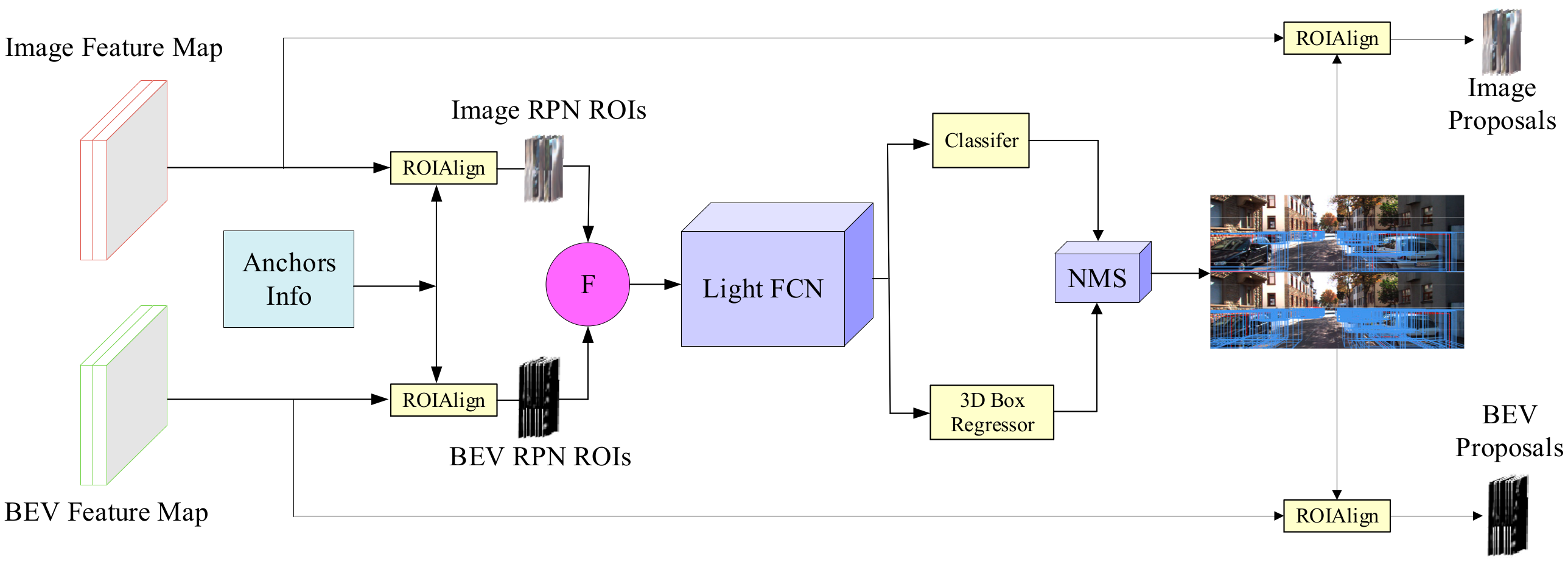
Referring to the RPN structure in Faster R-CNN, feature maps generated from both the image and BEV maps are fused and fed into a 3D proposal generator to regress the difference between the 3D anchors and the ground truth.

The 3D anchor was represented as an axis-aligned box encoding, where two clustering centers were selected to cluster the anchor size for vehicles in 3712 samples. At the same time, the orientation of each anchor was set to 0 and 90 degrees, i.e., there were four anchors in one location. As shown in Figure 6, the centers of the anchors were sampled at a stride of 0.5 m, eventually generating 89,600 anchors in BEV. The empty target anchors that did not contain LiDAR points were removed using preliminary screening, leaving about 21,000 anchors, as shown in the green box in Figure 6.

As shown in Figure 7, the features of each anchor were cropped and resized to 3 × 3 after dimensionality reduction via a 1 × 1 convolution. Then, the corresponding features from each view were fused via an element-wise operation. Finally, the fused feature vectors were passed into a light FCN network to output the categories of anchors and the axis-aligned box deviations between the anchors and the ground truth. The first k proposals based on the confidence score sorting were selected, and then the feature maps of the corresponding region from each proposal were cropped and resized to 7 × 7, which were finally fed to the second-stage refinement network.

The feature cropping and extraction operations of anchors and proposals have a great influence on the subsequent detection. RoIPooling [1] is the most commonly used operator; however, when extracting the feature of small-scale vehicles, the integer operation will lose a large amount of object information, and these quantization operations will lead to the extracted feature not matching the real object. RoIAlign [33] avoids integer operations by using floating-point arithmetic to accurately align the original image area and feature area of the object, and uses bilinear interpolation to regenerate the feature area accurately. Therefore, RoIAlign was exploited to generate the equal-sized features to improve the feature extraction accuracy of the anchors and proposals in this paper.

3.2.3. Refinement Network

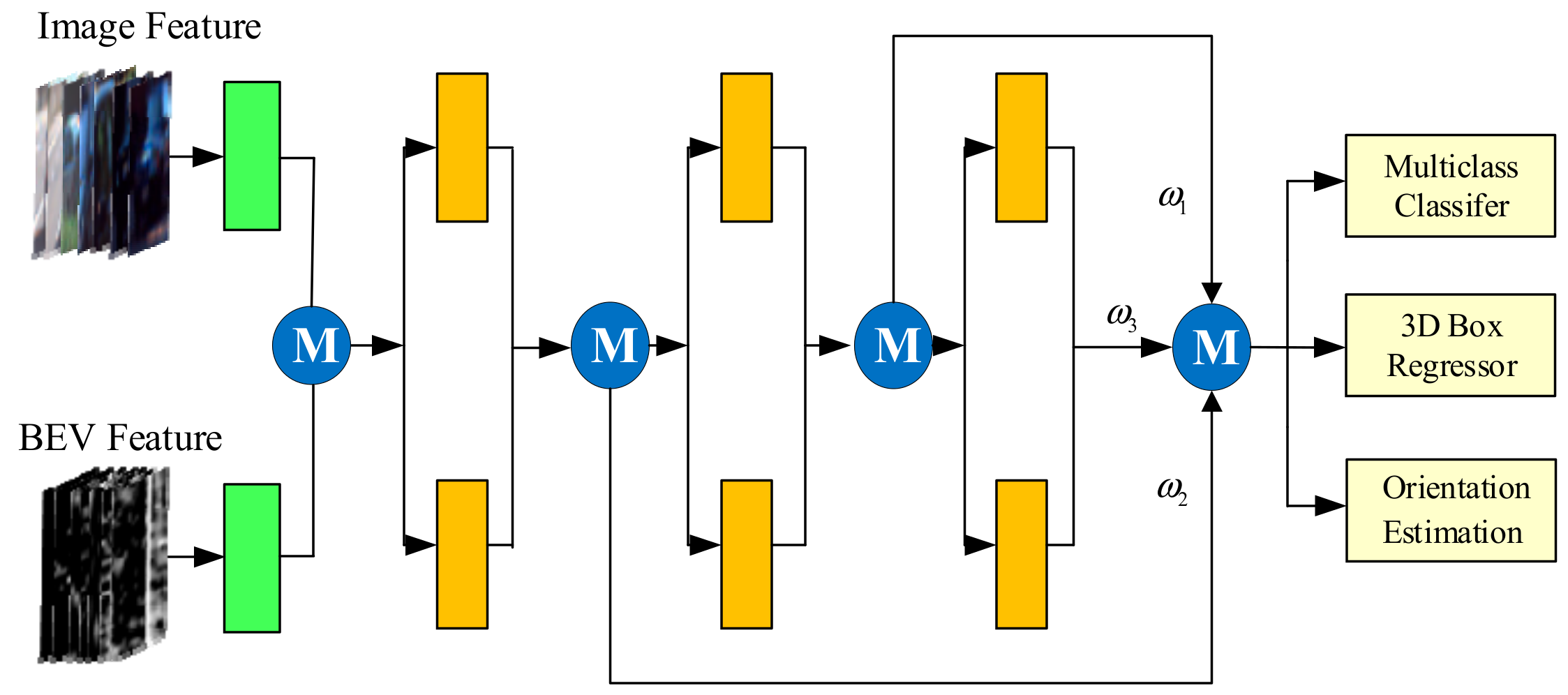
The features of each proposal were further fused to output the categories, locations, sizes, and orientations of the vehicles. At present, there are three fusion modes [6]: (1) early fusion, where features are merged at the beginning of processing; (2) late fusion, where features of each branch are processed separately and merged in the last stage; and (3) deep fusion, where features of each branch are mixed in different layers, resulting in a more general fusion scheme.

All three modes utilize fully connected layers that are connected step-by-step to process the fused feature and perform the 3D box regression, orientation estimation, and classification using the last layer only. Therefore, the cross-layer link structure in the feature extractor was also applied here to improve the efficiency of the fully connected parameters without increasing their numbers, as well as making full use of the characteristics of each layer. The cross-layer link structures under the three fusion modes are shown in Figure 8, Figure 9 and Figure 10.

Assuming that the fusion network had L layers, all fully connected layers were further fused to ensure that the final detection result depended on the parameters of each layer:

$$f_L={\omega }_1{f}_1^{\prime }\oplus \cdots \oplus {\omega }_{L-1}{f}_{L-1}^{\prime }\oplus {\omega }_L{f}_L^{\prime },$$

(3)

where $f_i^{\prime }$ represents the output of the features from ith fully connected layer, ${\omega }_i$ is the weight of the ith fully connected layer, and $\oplus$ is the fusion operation method used (e.g., concatenation, mean and maximum).

3.3. The Multi-Task Loss Function and Loss Weight Masks

The loss function of our network consisted of five parts: category loss and axis-aligned box regression loss in the 3D proposal generator network, category loss, and 3D bounding box regression loss and orientation estimation regression loss in the second refinement network, as shown in Equation (4). Among them, the value of the 2D intersection-over-union (IoU) in BEV between the anchors and ground truth was used to judge whether the anchor belonged to the background. Like the loss function in Faster R-CNN, the background anchor does not calculate the regression loss. The softmax function was used to calculate the category loss, and the Smooth L1 function was used to calculate the regression loss and orientation estimation loss.

$$Los{s}_{total}=los{s}_{pg\_cls}+los{s}_{pg\_reg}+los{s}_{3D\_cls}+los{s}_{3D\_reg}+los{s}_{3D\_ang}$$

(4)

The diversity of loss categories and computing methods make it difficult to optimize the network. In the experiments, the low regression accuracy in height dimension results in the AP_3D is more than 10% lower than the AP_BEV. Balancing the loss proportion of each optimization target in the total loss has a great impact on the final detection results.

Aiming toward solving the above problems, three weight masks were set in the loss function: one category loss weight mask for the total loss and two refined regression weight masks for the bounding box regression loss in the 3D proposal generator and the second-stage fusion network. For these three kinds of losses, we set the category weight mask to $\left[{\omega }_{cls},{\omega }_{reg},{\omega }_{ang}\right]$. In the 3D proposal generator network, anchors were encoded using the axis-aligned bounding box and are represented by the centroid $\left(c_x,c_y,c_z\right)$ and the axis-aligned dimensions $\left(l_x,w_y,h_z\right)$, as shown in Figure 11 (left). The regression target was the difference $\left(\Delta c_x,\Delta c_y,\Delta c_z,\Delta l_x,\Delta w_y,\Delta h_z\right)$ between a set of prior 3D anchor boxes and the ground truth boxes. Therefore, the weight mask was set to $\left[{\omega }_1^{pg},\dots ,{\omega }_6^{pg}\right]$. In the second-stage refinement network, the regression targets were the offsets of the four corners and the height from the ground plane between the proposals and the ground truth boxes $\left(\Delta x_1\dots \Delta x,\Delta y_1\dots \Delta y,\Delta h_1,\Delta h_2\right)$, as shown in Figure 11 (right). Therefore, the weight mask was set to $\left[{\omega }_1^{ref},\dots ,{\omega }_{10}^{ref}\right]$.

3.4. Training and Parameters Setting

We trained a network with an adaptive moment estimation (ADAM) optimizer for 120 K iterations and saved one model file per 1000 epochs. The initial learning rate and decay factor were set to 0.0001 and 0.8, respectively.

There were three fully convolutional layers in the 3D proposal generator, each with a 256-convolution kernel, and three fully connected layers in the refinement network, each with a parameter of 2048. The corresponding fusion weights were all defaulted to 1. The element-wise mean operation was used for the cross-layer link in the refinement network. The sizes of the 3D anchors were (l = 3.51 m, w = 1.58 m, h = 1.51 m) and (l = 4.23 m, w = 1.65 m, h = 1.55m). The loss category weight mask was set to [1:5:2], the regression weight mask in the 3D proposal generator was set to [1:1:3:1:1:3], and the regression weight mask in the refinement network was set to [1:…:1:3:3]. In addition, the dropout parameter in the refinement stage was set to 0.7.

4. Experiments and Results

In this section, we give the evaluation results of our FDCA network using the KITTI object detection benchmark, which is one of the most commonly used datasets in the driving scene. Like other 3D detection methods, 7481 labeled samples were split into a training set and a validation set at approximately a 1:1 ratio. Following the official classification criteria of KITTI, the samples were divided into “easy, moderate, and hard” cases. Our proposed networks were trained on the training set and the validation set was used to evaluate the performance of the trained networks. First, we compared the performance of the FDCA network with that of other published methods to prove the superiority of our proposed method. Then many ablation experiments were carried out to test the innovations this paper proposed.

4.1. 3D Vehicle Detection

In the research regarding 3D object detection, AP is best used to verify the performance of the method because it represents the performance not under a certain confidence threshold, but under all confidence thresholds. In practical application, a certain confidence threshold is usually selected (threshold when the recall is 0.1) to balance the accuracy rate and the false detection rate.

According to the official performance evaluation protocol of the KITTI 3D object detection benchmark, 3D vehicle detection results were evaluated using the AP_3D and AP_BEV at a 0.7 IoU threshold for three modes: easy, moderate, and hard.

We compared our proposed method with other fusion-based methods—MV3D, F-PointNet, and AVOD-FPN—and the comparison results were summarized in

Table 1. The performance comparison of our method and other methods using the KITTI validation set. AHS: average heading similarity, AP: average precision, Mod.: moderate.

Methods	Runtime	AP3D (%)			APBEV (%)			AHS (%)
		Easy	Mod.	Hard	Easy	Mod.	Hard	Easy	Mod.	Hard
MV3D	0.36 s	71.29	62.68	56.56	86.55	78.10	76.67	52.74	43.75	39.86
F-PointNet	0.17 s	83.76	70.92	63.65	88.16	84.02	76.44	-	-	-
AVOD-FPN	0.1 s	84.41	74.44	68.56	89.72	86.85	79.69	84.19	74.11	68.28
Our FDCA	0.11 s	85.38	76.82	69.34	89.76	87.05	79.88	85.28	76.57	69.13

.

It is shown that our proposed network outperformed all other fusion-based methods in terms of 3D object detection, with a noticeable margin of 0.97% 3D AP on the easy setting, 2.38% on the moderate setting, and 0.78% on the hard setting in comparison to the second-best performing method, AVOD-FPN. Similarly, the performance on orientation (average heading similarity, AHS) had the same tend. It was 1.09%, 2.46%, and 0.85% higher than that of AVOD-FPN for the three settings, respectively. However, for the AP_BEV, FDCA was not significantly higher than the AVOD-FPN (note that in AVOD-FPN, the performance of the AP_BEV is not provided; the results in Table 1 were obtained by running AVOD-FPN). This revealed that our innovations ultimately improved the performance of 3D object detection by improving the accuracy of the height regression. Meanwhile, the location error (average distance) of the detected vehicles was calculated to be 0.163 m. Compared with AVOD-FPN, which had the best performance in real-time, our architecture only slightly increased the runtime by 0.01 s on the GXT 1080Ti GPU. 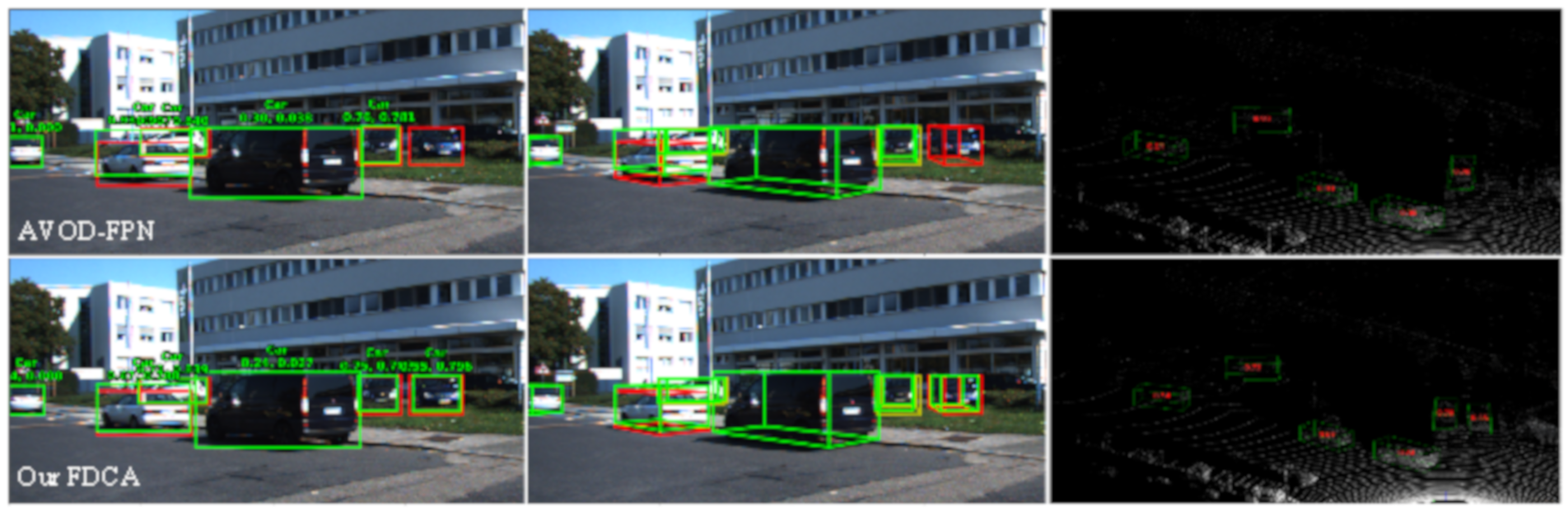Figure 12 shows the visual results of AVOD-FPN and our proposed method in both image and 3D point cloud space. It can be seen that the missing vehicle in AVOD-FPN was detected correctly in our architecture and the regression accuracy of the 3D bounding boxes of our architecture was higher than that of AVOD-FPN.

4.2. Ablation Studies

Many ablation experiments have been done in view of the innovation in this paper. The results are shown in

Table 2. Result of the ablation studies using a KITTI validation set at a 0.7 3D IoU.

Architecture	BEV Channel	Network	Loss Mask	Easy (%)		Moderate (%)		Hard (%)
				AP	AHS	AP	AHS	AP	AHS
Baseline Network	6	FPN+FC	✕	83.87	83.81	74.19	73.97	67.92	67.64
Seven-channel BEV Only	7	FPN+FC	✕	83.96	83.69	74.23	73.82	67.59	67.44
FDCA Only	6	FDCA	✕	85.04	84.98	75.16	74.96	68.44	68.21
Seven-channel BEV and FDCA	7	FDCA	✕	84.92	84.83	75.40	75.18	68.70	68.42
Our FDCA-Net	7	FDCA	✓	85.38	85.28	76.82	76.57	69.34	69.13

,

Table 3. Comparison results of fusion modes using the KITTI validation set.

Architecture	Fusion Mode	AP3D (IoU = 0.7) (%)
		Easy	Mod.	Hard
Baseline Network	Early	83.87	74.19	67.92
	Late	77.92	68.06	67.30
	Deep	84.27	74.05	68.13

and

Table 4. The comparison results of different weight masks.

Loss Weight Mask	AP3D (IoU = 0.7) (%)
	Easy	Mod.	Hard
[1:5:2], [1:1:1:1:1:1], [1:…:1:1:1]	84.92	75.60	68.70
[1:5:2], [1:1:2:1:1:2], [1:…:1:2:2]	84.65	75.46	68.66
[1:5:2], [1:1:3:1:1:3], [1:…:1:3:3]	85.38	76.82	69.34
[1:5:2], [1:1:4:1:1:4], [1:…:1:4:4]	84.66	76.33	69.00

. In the baseline network, the BEV map had six channels, as seen in References [6,7], where the feature extractor and refinement network adopted a traditional FPN network and fully connected network without loss weight masks.

4.2.1. The Fusion Mode

References [6,7,32] have different conclusions for three fusion modes. Schlosser et al. [34] considers that the late fusion mode is best, while MV3D [6] proposes the deep fusion mode, and AVOD [7] considers that the early fusion mode is best. Considering the divergence on the conclusions of fusion modes, the performance of different fusion modes was compared in this paper. The results are shown in the first to third rows of Table 3.

It can be concluded that the performance of the late fusion mode was only 68.06% AP on the moderate setting, which was evidently lower than that on the early and deep fusion mode. At the same time, the performance of the deep fusion mode was only higher by 0.4% and 0.21% than that of early mode on the easy and hard settings, respectively, and even lower by 0.14% on the moderate setting while undertaking more computation and having more parameters. Therefore, in the follow-up studies, early fusion mode was adopted in the second-stage refinement network.

4.2.2. BEV Map Representation

BEV is generated by projecting a raw point cloud into an overhead view, which inevitably causes information loss of objects. In Ku et al. [7], the BEV map consists of five local height channels and a density channel, while the seven-channel BEV map generated in our architecture preserved the global and local height information of the object. The results are shown in Table 2, where the seven-channel BEV map brings about a slight performance increase with 0.04% in the early setting and 0.29% on the deep setting (in the first and second rows). Similarly, the AP with a seven-channel BEV map outperformed that with a six-channel BEV by 0.24% on the basis of the proposed FDCA structure (in the third and fourth rows). This illustrates that our seven-channel BEV map was beneficial toward improving the detection performance for vehicles.

4.2.3. FDCA Structure

According to the comparison results in Table 2 (row 1 and row 3, row 2 and row 4), it can be seen that compared with the FPN + FC structure, the FDCA structure could achieve a large gain of 0.97% with a six-channel BEV and 1.17% with a seven-channel BEV on a moderate setting. In the easy and hard settings, the performance with the FDCA structure was also much higher than that with the FPN + FC structure. The performance of AHS had the same trend in the three settings. We also did a comparison experiment with FDCA and FPN + FC structures in the deep fusion mode. In particular, we reduced the parameter number of each fully connected layer by half, and the result shows that the performance with FDCA was higher than that with FPN + FC by 0.79%. This proves that the parameters of the cascaded fully connected layer were redundant, causing a performance degradation. The above experiments show that our proposed FDCA structure could greatly improve the detection performance of the network. Through continuous and deep fusion for features, the generalization ability of the network and the utilization efficiency of parameters were strengthened.

4.2.4. Loss Weight Mask

The design of the loss function has a great influence on the performance of the detection network, especially in the 3D object detection network, where more output targets make it difficult to optimize. The performance gap of the network in 3D space and the overhead view indicates that the height regression accuracy of the bounding boxes is poor. Therefore, in this section, we set different values for the three loss weight masks to increase the weight of height loss in the total loss. The network adopted the seven-channel BEV map and FDCA structure, and the results are shown in Table 4. For the three settings, the AP when the weight of the height information was set to 3 achieved a maximum gain of 0.46%, 1.22%, and 0.64% than that when the weight was set to 1. Therefore, based on the above experimental results, the weight value of high information was set to 3, and the results are also shown in the last line of Table 2. From Table 4, a conclusion can be drawn that the refined loss weight masks had a positive impact on the regression accuracy of the 3D bounding boxes.

4.2.5. Stability and Convergence

During the training stage, 120 training models were saved in total. We evaluated the 120 saved models using the validation set and obtained the AP of each model. The AP curves of the base network and ours are shown in Figure 13.

As can be seen, our methods had a higher performance than the base network. First, from the AP_3D of the first 30 models, our method converged faster than the base network. In addition, the AP_3D curve of the base network had a large fluctuation in the later stage, while the AP_3D curve of ours was more stable. We counted the AP_3D performance of the last 40 models for the base network and ours, and the average and standard deviation of the baseline network were 71.73% and 2.48%, while the value of our method without loss weight mask were 74.46% and 0.97%, and the value of our method with loss weight mask were 75.44% and 0.53% respectively. Thus, the proposed method not only improved the AP performance, but also the stability and convergence rate.

4.2.6. PR Curve

Figure 14 shows the precision versus recall (PR) curves for our methods and the base network. It can be seen that our FDCF outperformed the base network by a wide margin.

5. Conclusions

In this work, we proposed FDCA_Net, a 3D vehicle detector based on multi-sensory data fusion for autonomous driving scenarios. First, a seven-channel BEV map was generated to enhance its representational ability for vehicles by aggregating local and global features. Second, we proposed feature deep continuous aggregation structure, and the generalization ability of the network was improved by continuous features and deep fusion at different stages. Furthermore, a light fully convolutional network was adopted to reduce the computation load and memory requirements in the 3D proposal generator. Finally, three refined loss weight masks were added to the loss function to improve the regression accuracy of the 3D bounding boxes. The comparable experiments using the KITTI validation set show that FDCA_Net achieved a good detection accuracy with real-time performance. The ablation experiments showed that the point cloud representation, feature deep continuous aggregation structure, and refined loss weight mask proposed in this paper had a positive impact on improving the detection performance of 3D vehicles. At the same time, the convergence speed and stability were greatly improved. This method is applicable to the urban scene (maximum speed 60 km/h) and detects vehicles within 70 m in front of the vehicle. The limitation of this method is that it cannot work normally in some extreme scenarios; for example, it cannot collect high-quality images in low light, and there are many noise points in the point cloud data under rainy or snowy weather. Thus, further work will involve improving the robustness of the detection system, especially when a sensor fails under extreme scenes, which will involve distinguishing and managing it for the detection system to get reliable detection results.