Research on Combined Model Based on Multi-Objective Optimization and Application in Wind Speed Forecast

Abstract

Wind power is an important part of a power system, and its use has been rapidly increasing as compared with fossil energy. However, due to the intermittence and randomness of wind speed, system operators and researchers urgently need to find more reliable wind-speed prediction methods. It was found that the time series of wind speed not only has linear characteristics, but also nonlinear. In addition, most methods only consider one criterion or rule (stability or accuracy), or one objective function, which can lead to poor forecasting results. So, wind-speed forecasting is still a difficult and challenging problem. The existing forecasting models based on combination-model theory can adapt to some time-series data and overcome the shortcomings of the single model, which achieves poor accuracy and instability. In this paper, a combined forecasting model based on data preprocessing, a nondominated sorting genetic algorithm (NSGA-III) with three objective functions and four models (two hybrid nonlinear models and two linear models) is proposed and was successfully applied to forecasting wind speed, which not only overcomes the issue of forecasting accuracy, but also solves the difficulties of forecasting stability. The experimental results show that the stability and accuracy of the proposed combined model are better than the single models, improving the mean absolute percentage error (MAPE) range from 0.007% to 2.31%, and the standard deviation mean absolute percentage error (STDMAPE) range from 0.0044 to 0.3497.

1. Introduction

In recent years, wind energy has become the focus of managers and researchers in the energy field, due to the advantages of wind power, such as renewability and cleanliness.

In 2016, the global installed capacity of wind power exceeded 54 GW. This installed capacity is distributed between 90 countries, which have an installed capacity of more than 10 GW, with 29 countries having an installed capacity of 1 GW [1]. Cumulative installed capacity increased by 12.6%, and accumulated capacity reached 486.8 GW. In the United States, more than 53,000 wind turbines operate, generating more than 84.1 GW of electricity in 41 states [2]. On the other side of the globe, wind power may become China's second largest power source by 2050 [3].

Accurate forecasting of wind speed is an important prerequisite for using wind power due to the following reasons: 1) it reduces rotating and operating costs of wind-farm equipment; 2) it helps dispatching departments to adjust their plans in time; 3) it reduces the impact on the entire power grid; 4) it effectively reduces or avoids the negative impact of wind farms on the power system, and 5) it improves the ability of wind power in power market competition.

However, because of the chaotic and random fluctuations of wind speed, it is a challenging and difficult task to obtain satisfactory wind-speed forecasting results [4,5,6]. To have satisfying results and reduce errors, and improve the accuracy and stability of the forecasting results, various wind-speed forecasting methods have been proposed and developed by former researchers. The methods can be classified in four categories: 1) physical models; 2) statistical models; 3) artificial-intelligence models; and 4) spatial-correlation models [7].

The common physical models include weather research and forecast, the consortium for small-scale modeling, and mesoscale model 5 (MM5) [8]. These methods are based on physics and the atmosphere, and forecast wind speed with additional background information [8]. Statistical models include the fuzzy methods [9], Autoregressive Moving Average (ARMA) model [10], the Autoregressive Integrate Moving Average (ARIMA) model [11,12], and the grey model [13], combined with neurofuzzy techniques [14] and Markov chains [15]. Statistical methods aim to mine the relationship between historical data and establish prediction models, including traditional statistical and machine-learning models, to describe the potential sampling of wind-speed forecasting [16]. In recent years, because of their powerful nonlinear character, many artificial-intelligence forecasting methods, such as artificial neural networks (ANN) [17,18,19,20,21,22,23,24,25] and support vector machines (SVM) [26,27], have been widely applied to wind-speed forecasting. The wind speed of the spatial relationship between different sites is considered in spatial-correlation models [28] to forecast wind speed.

However, these four categories of methods have disadvantages because of their character: 1) physical models need accurate numerical weather-prediction data and detailed information of wind-farm locality, input parameters, and data acquisition. Processing and calculation are complex [29,30]; 2) traditional statistical models can address forecasting with linear trends well, but times-series wind speed is always random, chaotic, and nonlinear, and the performance of these models does not satisfy researchers and managers; 3) although artificial-intelligence forecasting methods have some advantages, due to their nonlinear mapping capability compared with traditional statistical models, their main disadvantages and shortcomings are that they are easy to reach local optimal values, and they suffer from overfitting and slow convergence [31]; 4) spatial-correlation methods should consider many influential factors, such as the relationship of the time-series wind-speed data between different sites, original data from several stations, and if the time-series wind speed of the forecasting point and its neighbors is used for forecasting [28].

To overcome the problem of forecasting accuracy and stability and take advantage of single models, a combined model based on multi-objective optimization and combined theory is proposed by us to overcome their defects, including low accuracy and weak stability. Because wind-speed forecasting is a complex study, single-objective optimization is not enough to solve the wind-speed forecasting problem. Solving the single-objective optimization problem (SOP) is a direct task, but multiple-objective problems (like the wind-speed forecasting problem) are often complex, and objective functions are competing (or conflicting) with each other. Due to this reason, there is no single optimal solution, commonly known as a series of Pareto-optimal solutions, which simultaneously optimize all objective functions. A set of optimal solutions, called a Pareto-optimal Set (PS), of which mapping in the target space is named the Pareto front (PF), and not a single optimal solution, is the goal of solving the multiple-objective optimization problem (MOP). In MOPs, the favored solution from the PS is chosen by researchers, but not the optimal solution. Obviously, it is difficult to select one objective function from a number of objective functions and ensure that the selected objective function can achieve a lower mean absolute percentage error (MAPE) and stronger stability. Due to these reasons, multiple-objective optimization can solve the low accuracy and weak stability of the wind-speed forecasting problem through simultaneously searching the goal of multiple functions.

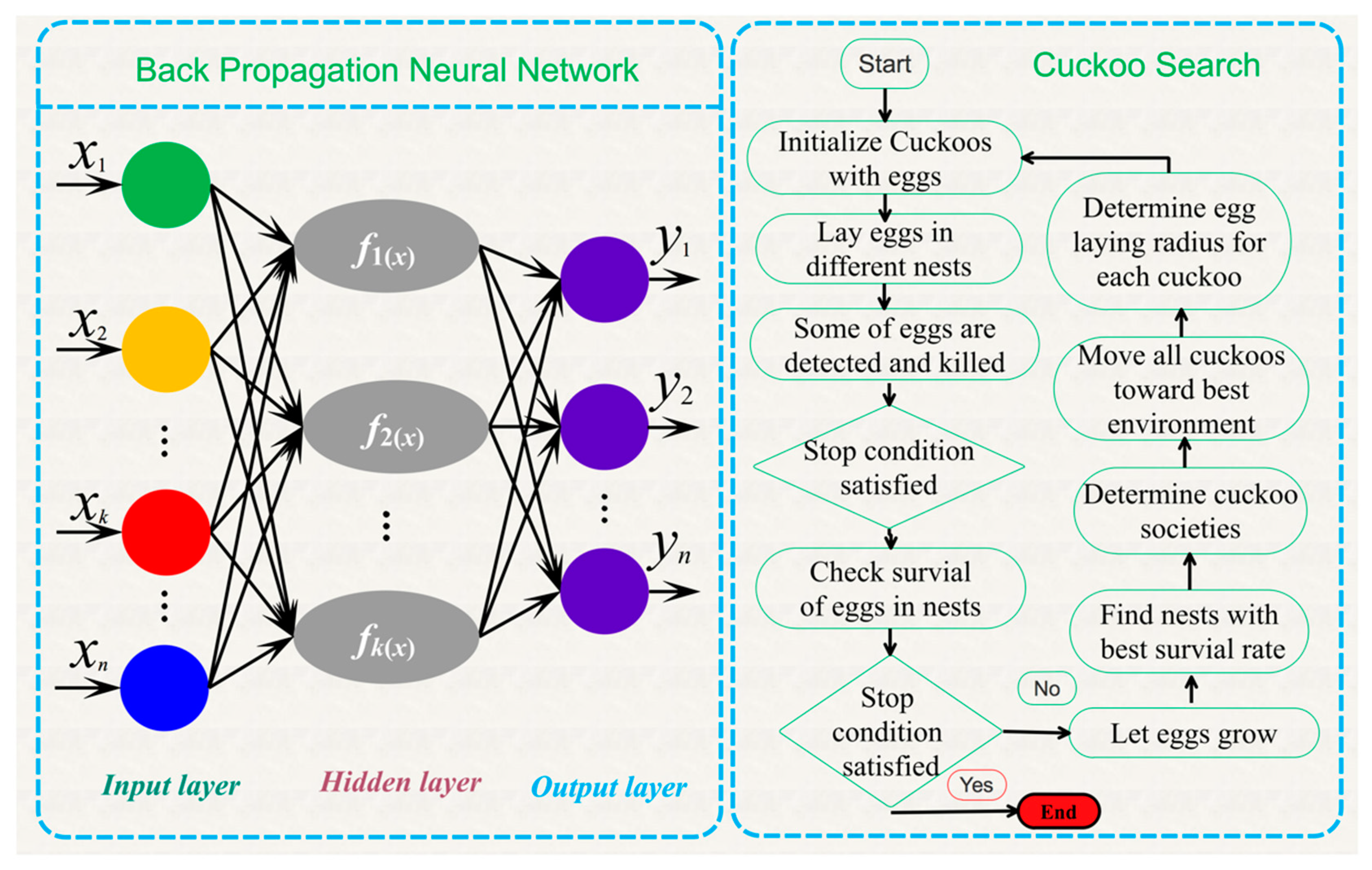
In this paper, a new combined model [32] that integrates nonpositive constraint theory [33], four branch models, including two nonlinear hybrid neural networks (Cuckoo Search-Back-Propagation Neural Network (CS-BPNN) and DE-Online Extreme Learning Machine (DE-OSELM)), two linear models (ARIMA and HW), and a nondominated sorting genetic algorithm (NSGA-III) [34], which optimizes the weights of the branch models, is proposed in this paper. Ten-minute time-series wind-speed data from three wind-farm sites were applied to examine our proposed model. We also chose three combined models with two objective functions to test its performance.

The major contributions and innovations of this paper are as follows:

1. According to the observed time-series wind-speed data, the trajectory matrix was constructed, decomposed, and reconstructed to extract signals representing different components of the original time series, such as long-term trend signals, periodic signals, and noise signals, so that the structure of the time series could be analyzed and used for further forecasting.

2. Our proposed combined model is based on MOP theory, which can obtain both accuracy and stability. The wind-speed forecasting problem is a MOP, so the theory overcomes the difficulty of selecting one objective function from multiple functions to obtain higher precision and stronger stability.

3. Due to the wind-speed data having both linear and nonlinear characteristics, linear models (ARIMA and HW) and nonlinear models (BPNN) and OSELM) were chosen to be the branch models of our proposed combined model. The combination of these two kinds of models can solve the wind-speed forecast problem with both linear and nonlinear characteristics.

4. Our novel developed combined model with three objective functions, which can be applied to forecast wind speed, is proposed in this paper. As compared with other models, the proposed model not only guarantees accuracy, but also has strong stability. The results of the experiments mean that the proposed integrated combined model is a more effective model for wind-speed forecasting and wind-farm management.

5. The forecasting performance of the combined model was evaluated scientifically and comprehensively. The evaluation system used five experiments and four performance metrics to effectively evaluate the forecasting accuracy and stability of the proposed combined model.

The remainder of the paper is arranged as follows. The strategy of the proposed combined model is shown in Section 2. Singular-spectrum analysis is presented in Section 3. Nonlinear back propagation, an extreme learning machine neural network, two linear models, autoregressive integrated moving average and Holt–Winters, heuristic algorithms, and the optimization procedure are introduced in Section 4. In Section 5, we show our proposed combined model. In Section 6, forecasting performance metrics, the forecasting results of individual models and of the proposed combined model, and comparisons are discussed, and the views and results of the entire paper are summarized. Finally, Section 7 concludes the study.

2. Strategy of Our Proposed Combined Model

(1) Preprocessing the time-series wind-speed data with denoising and reconstruction from China.

(2) Setting the train data and test data according to the character of the time-series wind-speed data; the interval of each two data items is ten minutes.

(3) Two kinds of models were selected as single models to build the combined model. The linear models include ARIMA and HW, and the nonlinear models include CS-BPNN and DE-OSELM, which were optimized by cuckoo search and differential evolution. The parameter values are shown in

Table 1. Four metrics.

Metric	Definition	Equation
AE	The average forecast error of n times forecast results	$\mathbf{AE}=\frac{1}{N}{{\displaystyle \sum }}_{n=1}^N(y_n-{\widehat{y}}_n)$
MAE	The average absolute forecast error of n times forecast results	$\mathbf{MAE}=\frac{1}{N}{{\displaystyle \sum }}_{n=1}^N|y_n-{\widehat{y}}_n|$
MSE	The average of the prediction error squares	$\mathbf{MSE}=\frac{1}{N}{{\displaystyle \sum }}_{n=1}^N{(y_n-{\widehat{y}}_n)}^2$
MAPE	The average of absolute percentage error	$\mathbf{MAPE}=\frac{1}{N}{{\displaystyle \sum }}_{n=1}^N|\frac{y_n-{\widehat{y}}_n}{y_n}|\times 100\%$

.

(4) Building a combined forecasting system model, which is based on nonpositive constraint theory, NSGA-III, which optimizes the weights of the branch models and four single models, which are mentioned before.

(5) Forecasting results were evaluated, and testing of the combined model is at the end.

3. Results

The denoising process consists of four steps, embedding, singular-value decomposition, grouping, and diagonal averaging [35]. According to the observed time-series wind-speed data and these four steps, the trajectory matrix was constructed. The trajectory matrix was decomposed and reconstructed to extract signals representing different components of the original time series, such as long-term trend signals, periodic signals, and noise signals. In order to obtain satisfying results, the noise signals were abandoned. The detailed process is as follows:

(1) Embedding:

Form the trajectory matrix of the series X, which is the $L\times K$ matrix:

$$X=\left[x_1,\cdots {,x}_N\right]{=(x}_{\mathit{ij}}{)}_{i,j=1}^{L,K}=\left[\begin{array}{ccccc}{x}_1& x_2& x_3& \cdots & x_K\\ x_2& x_3& x_4& \cdots & x_{K+1}\\ x_3& x_4& x_5& \cdots & x_{K+2}\\ ⋮& ⋮& ⋮& \ddots & ⋮\\ x_L& x_{L+1}& x_{L+2}& \cdots & x_N\end{array}\right]$$

(1)

where $X={(x_1, \cdots {, x}_{i+L-1})}^T,(1<i<K)$ are lagged vectors of size L. Matrix X is a Hankel matrix that means that X has equal elements $x_{\mathit{ij}}$ on the anti-diagonals i +j=const.

(2) Singular-Value Decomposition:

Perform the singular value decomposition (SVD) of trajectory matrix X. Set ${S = \mathit{XX}}^T$ and denote by ${\lambda }_1,\cdots {,\lambda }_L$ the eigenvalues of S taken in the decreasing order of magnitude ${\lambda }_1\ge \cdots \ge {\lambda }_L\ge 0$, and by $U_1{,\dots ,U}_L$ the orthonormal system of the eigenvectors of matrix S corresponding to these eigenvalues.

Set $d = \mathit{rankX} = \mathit{max}\left\{{i, \mathrm{such} \mathrm{that} \lambda }_i > 0\right\}$ (note that d = L for a typical real-life series) and $V_i{ = X}^{T}U/\sqrt{{\lambda }_i},(i = 1,\dots ,d)$. In this notation, the SVD of trajectory matrix X can be written as ${\mathit{X} =\mathit{X}}_1+ \cdots { +\mathit{X}}_N$.

Where ${\mathit{X}}_i = \sqrt{{\lambda }_i}{U}_i{V}_i{}^T$ are matrices having rank 1; these are called elementary matrices. Collection $(\sqrt{{\lambda }_i}{, U}_i{, V}_i{}^T)$ is the ith eigentriple (ET) of the SVD. Vectors $U_i$ are the left singular vectors of matrix X, and numbers $\sqrt{{\lambda }_i}$ are the singular values and provide the singular spectrum of X; this gives the name to SSA. Vectors $V_i\sqrt{{\lambda }_i}{ = X}^T{U}_i$ are the vectors of principal components (PCs).

(3) Eigentriple grouping:

Partition set of indices $\left\{1, \dots , d\right\}$ into m disjoint subsets $I_1,\cdots {,I}_m$.

Let $I = \left\{i_1,\cdots {,i}_p\right\}$. Then, resultant matrix ${\mathit{X}}_I$ corresponding to group I is defined as ${\mathit{X} =\mathit{X}}_{I_1}+\cdots {+\mathit{X}}_{I_m}$. The resultant matrices are computed for the groups, and the grouped SVD expansion of X can now be written as ${\mathit{X} = \mathit{X}}_{I_1}{+\dots +\mathit{X}}_{I_m}$.

(4) Diagonal averaging:

Each matrix ${\mathit{X}}_{I_j}$ of the grouped decomposition is hankelized, and then the obtained Hankel matrix is transformed into a new series of length N using the one-to-one correspondence between Hankel matrices and the time series. Diagonal averaging applied to a resultant matrix ${\mathit{X}}_{I_k}$ produces a reconstructed series ${\tilde{X}}^{(k)}=({\tilde{X}}_1^{(k)},\cdots ,{\tilde{X}}_N^{(k)})$. In this way, the initial series $x_1,\cdots ,x_N$ is decomposed into a sum of m reconstructed subseries:

$$x_n={\displaystyle \sum }_{k=1}^m{\tilde{x}}_n^{(k)}, (n=1,2,\dots ,N)$$

(2)

This decomposition is the main result of the SSA algorithm. The decomposition is meaningful if each reconstructed subseries could be forecast as a part of either a trend, some periodic component, or noise.

The pseudocode for denoising is provided in Appendix A, Algorithm 1.

4. Methods and Heuristic Algorithm

The linear and nonlinear models selected to build the combined system are shown in this section. The heuristic algorithm, cuckoo search, and differential evolution to optimize BPNN and OSELM are also introduced in this section.

4.1. Nonlinear Models

Because of the character of wind-speed data, nonlinear models can obtain excellent performance in forecasting. In this paper, two models, BPNN and ELM, were selected from nonlinear models and the parameter was optimized by the algorithm to obtain better performance.

4.1.1. Back-Propagation Neural Network (BPNN) Model

BPNN is a type of multilayer feed-forward neural network with a wide variety of applications. It is based on a gradient-descent method that minimizes the sum of the squared errors between actual and desired output values. The transfer function is of the neuron type. The output function is between 0 and 1, and can transform input to output for continuous nonlinear mapping [36].

The topology of the BPNN is as follows:

$$X^{\prime }=\left\{X^{\prime }i\right\}=2\times \frac{X_i-X_{i\min }}{X_{i\max }-X_{i\min }}-1,(i=1,2,\dots ,n),X^{\prime }\subset \left[-1,1\right]$$

(3)

where $X_{\min }$ and $X_{\max }$ are the minimum and maximum value of the input array or output vectors, and X′i denotes the real value of each vector.

Step 1. Calculate outputs of all hidden layer nodes:

$$y_j=f({\displaystyle \sum }_i{w}_{ji}{x}_i{+b}_j)=f({net}_j) (i =1,\dots ,n ; j =1,\dots ,2n)$$

(4)

$${\mathit{net}}_j={\displaystyle \sum }_i{w}_{\mathit{ji}}{x}_i{+b}_j, (j = 1,\dots ,2n)$$

(5)

where the activation value of node j is ${\mathit{net}}_j$, $w_{\mathit{ji}}$ representing the connection weight from input node i to hidden node j, $b_j$ represents the bias of neuron j, $y_j$ represents the output of hidden layer node j, and f is the activation function of a node, which is usually a sigmoid function.

Step 2. Calculate the output data of the neural network:

$$O_1{ = f}_0({\displaystyle \sum }_j{w}_{0j}{y}_i{+b}_0), (i = 1,\dots ,2n)$$

(6)

where $w_{0j}$ represents the connection threshold from hidden node j to the output node, $b_0$ represents the bias of the neuron, $O_1$ represents the output data of the network, and $f_0$ is the activation function of the output layer node.

Step 3. Minimize the global error via the training algorithm:

$$\mathit{Mean} \mathit{Square} \mathit{Error} = \frac{1}{m}{\displaystyle \sum }{(O_1-Z)}^2$$

(7)

where Z represents the real data vector of the output, m represents the number of output.

4.1.2. CS Algorithm

CS, which was proposed by Yang and Deb [37] in 2009, is derived from the action of cuckoos laying their eggs in other birds’ nests to let those birds hatch the eggs for them. However, once the host birds discover the cuckoo eggs, the host birds throw them away or abandon their nests and rebuild a new nest elsewhere. The CS algorithm is constructed based on three assumptions: a) only one egg is randomly laid by each cuckoo in a selected nest; b) the following generations would begin in the best nest; and c) it is a constant of the number of available host nests, and the probability value of the host bird discovering the egg laid by a cuckoo is p, which has the range of 0 to 1. In CS, every nest stands for a solution. The steeps of BPNN optimized by CS are shown in Figure 1.

4.1.3. OSELM

An Extreme Learning Machine (ELM) is a simple and effective single hidden-layer feed-forward neural network proposed by Huang et al. [38]. In many practical applications, however, learning is a continuous process. For this reason, Liang et al. proposed an online learning algorithm, the OSELM [39].

For different N training sample Z, $Z=\left\{{(x}_i{, t}_i)|i=1,\dots ,N\right\}$, where $x_i{=[x}_{i1}{, x}_{i2},\cdots {,x}_{\mathrm{in}}]\in R^n$, $t_i{=[t}_{i1}{, t}_{i2},\cdots {, t}_{\mathrm{im}}]\in R^m$, ELM with L hidden layer nodes, and g(x) activation function can approximate arbitrary N samples with zero errors by arbitrarily specifying $a_j$ and $b_j$, which can be expressed as follows:

$$O_i = {\displaystyle \sum }_{j=1}^L{\beta }_{j}g(a_j{,b}_j{,x}_i){= t}_i$$

(8)

where $a_j$ is the input weight, $b_j$ is the threshold of hidden layer nodes,${ x}_i$ is the input vector, $O_i$ is the output vector, and beta β_j is the output weight ${\beta }_{L\times m}{= [\beta }_1{, \beta }_2, \cdots {, \beta }_L{]}^T$.

Formula (8) can be simplified as:

$$H\beta = T$$

(9)

where, ${\beta }_{L\times m}{= [\beta }_1{, \beta }_2, \cdots {, \beta }_L{]}^T$, $T_{N\times m}{= [T}_1{, T}_2, \cdots {, T}_N{]}^T$, and H is hidden layer output matrix. $H(a_1,\cdots {,a}_L{; b}_1,\cdots {,b}_L{;x}_1,\cdots {,x}_N) ={\left[\begin{array}{ccc}{g(a}_1{, b}_1{, x}_1)& \cdots & {g(a}_L{, b}_L{, x}_1)\\ ⋮& \ddots & ⋮\\ {g(a}_1{, b}_1{, x}_N)& \cdots & {g(a}_L{, b}_L{, x}_N)\end{array}\right]}_{N\times L}$. Column J of H represents the output of the j hidden layer node for input $x_1{, x}_2, \cdots {,x}_N$.

After the pseudoinverse matrix is incorporated, the least-squares solution of the above linear system is:

$$\widehat{\beta }=(H^T{H)}^{-1}{H}^{T}T$$

(10)

Based on a recursive least-squares algorithm, the algorithm flow of OSELM can be described as follows:

(1) Initialization Stage

Given activation function g, the number of hidden layer nodes is L. A small training set is given to initialize the network and obtain the initial value. The output weight value is ${\beta }^{(0)}$. Take k = 0, where k is the number of data segments sent to the network, which is represented.

(2) Online Learning Stage

Given the k + 1 data segment, calculate output weight beta ${\beta }^{(k+1)}$, take k = k + 1, then return to the online learning stage, and constantly update the calculated output weight until data learning is completed.

4.1.4. Differential Evolution

The differential-evolution algorithm is a parallel, direct, and random-search algorithm based on group evolution [40]. Firstly, the population can be randomly initialized in the feasible solution space of the problem. The population can be represented by NP (population size) D (number of decision variables), dimension parameter $x_{hl}$, where h = 1, 2, …,NP, l = 1, 2,…, D.

Two different individual vectors are randomly selected and subtracted to generate difference vectors. The difference vectors are weighted and added to the third random selected individual vectors to generate variation vectors. This operation is called variation. Utilizing Formula (11) to implement a mutation operation on each individual $x_h^t$ at t-time, the corresponding mutation individual $v_h^{t+1}$ is obtained, that is:

$$v_h^{t+1}{= x}_{r_1}^t+K(x_{r_2}^t{- x}_{r_3}^t)$$

(11)

where, $r_1{,r}_3{,r}_3\in \left\{1,2,\dots , NP\right\}$ are different, and different to h.

The variation vector is mixed with the target vector to generate test vectors. This process is called a crossover. Formula (12) is used to cross-operate $x_h^t$ with variant individual $v_h^{t+1}$ generated by Formula (11) to generate experimental individual $u_h^{t+1}$, that is:

$$u_h^{t+1} = \{\begin{array}{cc}{v}_{h,l}^{t+1},& \mathrm{If} (\mathit{rand}(l) \le \mathit{CR}) \mathrm{or} l=\mathit{rnbr}(h);\\ x_{h,l}^t,& \mathrm{otherwise}.\end{array}$$

(12)

where, rand (l) is a uniformly distributed random number in the range of [0,1]; CR is a cross probability in the range of [0,1]; and rnbr (h) is a random variable in the range of {1, 2, …, D}.

If the fitness of the test vector is better than that of the target vector, the next generation is formed by replacing the target vector with the test vector. This operation is called selection. Fitness functions J of $u_h^{t+1}$ and $x_h^t$ were compared by Formula (6). For the minimization problem, the individual with a low fitness function value was selected as the individual $x_h^{t+1}$ of the new population, that is:

$$x_h^{t+1}=\{\begin{array}{cc}{u}_h^{t+1},& \mathrm{if} J(u_h^{t+1})<J(x_h^t);\\ x_h^t ,& \mathrm{otherwise}.\end{array}$$

(13)

where J is the fitness function. The Figure 2 shows the flow chart of hybrid OSELM.

4.2. Linear Models

Although wind-speed data are usually nonlinear, according to our test in Section 6.1, the time-series wind-speed data also have a linear character. We can say that the linear models used to build the combined system are correct and appropriate. In this section, two linear models are briefly introduced.

4.2.1. ARIMA

The ARIMA model is one of the most popular forecasting models [41]. The ARIMA model can be expressed as follows:

$$y_t = {\varphi }_1{y}_{t-1}+{\varphi }_2{y}_{t-2}+\cdots +{\varphi }_p{y}_{t-p}{+ \epsilon -\theta }_q{\epsilon }_{t-q}$$

(14)

where $y_i(i=1,2,\dots ,t)$ is the actual value, ${\epsilon }_i(i=1,2,\dots ,t)$ is the random error at time t, ${\varphi }_i$ and ${\theta }_i$ represent the coefficients, and p and q are internumbers that are often referred to as autoregressive and moving average polynomials, respectively.

4.2.2. Holt–Winters (HW)

The output of the HW method is written as $F_{t+m}$, an estimate of the value of x at time t + m, m > 0 based on the raw data up to time t; suppose we have a sequence of observations {$x_t$}, beginning at time t = 0 with a cycle of seasonal change of length L. The formula and recursive updating equations are the following:

$$F_{t+m}{=s}_t{+\mathit{mb}}_t{+c}_{t-L+1+(m-1)}$$

(15)

where $s_t = \alpha (x_t{-c}_{t-L})+(1-\alpha )(s_{t-1}{+b}_{t-1})$, $b_t=\beta (s_t{-s}_{t-1}) + (1-\beta )b_{t-1}$, $c_t = \gamma (x_t{-s}_{t-1}{-b}_{t-1})+(1-\gamma )c_{t-L}$, α is the data-smoothing factor, β is the trend-smoothing factor, γ is the seasonal change-smoothing factor, and these three parameters are between 0 to 1. {$s_t$} and {$b_t$} represent the smoothed value of the constant part for time t and the sequence of best estimates of the linear trend that are superimposed on the seasonal changes, respectively. {$c_t$} is the sequence of seasonal-correction factors [42].

5. Our Proposed Combined Model

The combined model theory, MOPs, our proposed combined system with three objective functions, and the compared combined model with two objective functions are presented in this section. The flowchart is shown in Figure 3.

5.1. Combined-Model Theory

The forecasting model based on combination, which was initiated by Bates and Granger [32], has long been considered as representing an improvement over individual models and also as an efficient and simple way to perfect forecasting accuracy and stability. A new combined system that consolidates several neural networks, NSGA-III, and nonpositive constraint theory [34] was successfully proposed in this paper.

Definition 1.

Let ${\hat{x}}_{j,t}$ denote the unbiased out-of-sample forecast for $x_t$, which is obtained by thejth individual model. Then, the combined output at time t of the combining methods has the following weighted average form [43,44]:

$${\widehat{x}}_{c,t}={{\displaystyle \sum }}_{j=1}^m{w}_j{\widehat{x}}_{j,t}, t=1,2,\dots$$

(16)

where ${\hat{x}}_{c,t}$ is the combined output, m is the number of the component models, and $w_j$ is the weight on thejth component model. These weights have no limitation in the range of [0,1]. The experiment results show that the combination model can obtain desirable results when the weight vector has a value in the range of [–2,2] [33].

5.2. Multiobjective Optimization Problem

Generally, MOPs can be classified into two groups: constrained and unconstrained problems. Constrained problems with J inequality and K equality constraints can be formulated as:

Definition 2.

$$\mathrm{Minimize} F(x) = {(f_1(x),f_2(x), \cdots ,{ f}_M(x) )}^T$$

(17)

$$\begin{array}{c}s.t{. g}_j(x) \ge 0, j=1,2, \dots , J,\\ h_k(x) = 0, k = 1,2, \dots , K,\end{array} x \in \Omega .$$

(18)

whereMis the number of objectives, and $M \ge 4$, and${x=(x}_1{, x}_2, \cdots {, x}_n{)}^T$is the decision vector, wherenis the number of decision variables. In MOP (1), $\Omega = {{\displaystyle \prod }}_{i=1}^n\left[x_i^L{, x}_i^U\right]\subseteq R^n$is called the decision space, where$x_i^L$and$x_i^U$are the lower and upper bounds of the decision variable$x_i$, respectively.

When the inequality and equality constraints in MOP (1) were omitted, then the unconstrained (with box constraints only) problems were obtained, which can be stated as follows:

Definition 3.

$$\mathrm{Minimize} \mathit{F}(x) = {(f_1(x){,f}_2(x), \cdots {, f}_M(x) )}^T$$

(19)

$$\begin{array}{c}s.t.\end{array} x \in \Omega .$$

(20)

In order to solve MOP, the NSGA-III is presented in the next section.

5.3. Introduction of Objective Functions and NSGA-III

Since wind-speed prediction is not a single-objective problem, it is necessary to consider multiple objectives to obtain both accuracy and stability. In this part, we show a multi-objective optimization algorithm that optimizes the weights of four models and three proposed objective functions to comprehensively consider this problem.

5.3.1. Objective Functions

In this paper, we chose three functions to be the objective functions.

(1) The Theil Inequality Coefficient (TIC) can be indicated as follows:

$$\mathrm{TIC}(\widehat{\mathit{Y}}, \mathit{Y})=\frac{\sqrt{\frac{1}{N}{{\displaystyle \sum }}_{i=1}^N{({\widehat{y}}_i-y_i)}^2}}{\sqrt{\frac{1}{N}{{\displaystyle \sum }}_{i=1}^N{{\widehat{y}}_i}^2}+\sqrt{\frac{1}{N}{{\displaystyle \sum }}_{i=1}^N{y_i}^2}}$$

(21)

TIC is always between 0 to 1; a lower numerical value is equal to better performance.

(2) Root mean squared error (RMSE). A smaller absolute value of RMSE $(\hat{\mathit{Y}}, \mathit{Y})$ indicates a more accurate forecasting performance of the system. It can be defined as follows:

$$\mathrm{RMSE}(\widehat{\mathit{Y}}, \mathit{Y})=\sqrt{\frac{1}{N}{{\displaystyle \sum }}_{i=1}^N{({\widehat{y}}_i-y_i)}^2}$$

(22)

(3) MAPE can be represented as:

$$\mathrm{MAPE}(\widehat{\mathit{Y}}, \mathit{Y})=\frac{1}{N}{{\displaystyle \sum }}_{i=1}^N\frac{\left|{\widehat{y}}_i-y_i\right|}{y_i}$$

(23)

The lower MAPE ($\widehat{\mathit{Y}}, \mathit{Y}$) is, the more accurate the system.

Thus, in this combined system, the fitness function for the accuracy and stability objectives can be defined as follows:

$$\mathbf{Minimize}=\{\begin{array}{c}{f}_1=\mathrm{TIC}(\widehat{\mathit{Y}}, \mathit{Y})\\ f_2=\mathrm{RMSE}(\widehat{\mathit{Y}}, \mathit{Y})\\ f_3=\mathrm{MAPE}(\widehat{\mathit{Y}}, \mathit{Y})\end{array}$$

(24)

5.3.2. NSGA-III

A random population of size N and a set of widely distributed prespecified M-dimensional reference points H on a unit hyperplane, which is placed in a manner so that it intersects each objective axis at one, having a normal vector of ones covering the entire $R_{+}^M$ region, were initialized by NSGA-III [45]. The more detailed description of NSGA-III is shown in the Appendix A.

5.4. Compared Combined Models with Two Objective Functions

There are three two-object-function models that were chosen to compare with our combined system:

(1) Combined model with Object Function (21) and (22);

$$\mathbf{Minimize}=\{\begin{array}{c}{f}_1=\mathrm{TIC}(\widehat{\mathit{Y}}, \mathit{Y})\\ f_2=\mathrm{RMSE}(\widehat{\mathit{Y}}, \mathit{Y})\end{array}$$

(25)

(2) Combined model with Object Function (21) and (23);

$$\mathbf{Minimize}=\{\begin{array}{c}{f}_1=\mathrm{TIC}(\widehat{\mathit{Y}}, \mathit{Y})\\ f_2=\mathrm{MAPE}(\widehat{\mathit{Y}}, \mathit{Y})\end{array}$$

(26)

(3) Combined model with Object Function (22) and (23).

$$\mathbf{Minimize}=\{\begin{array}{c}{f}_1=\mathrm{RMSE}(\widehat{\mathit{Y}}, \mathit{Y})\\ f_2=\mathrm{MAPE}(\widehat{\mathit{Y}}, \mathit{Y})\end{array}$$

(27)

6. Experiments

Some performance metrics must be described to comprehensively understand the model characteristics. Diebold-Mariano and forecasting effectiveness were used in this study. Four experiments are given in this section to text the data and our proposed combined system.

6.1. The Performance Metric

Some performance metrics must be described to comprehensively understand the model characteristics. Four metrics, that is, AE, MAE, MSE, and MAPE, are shown in Table 1.

6.1.1. Diebold Mariano test

A comparison test, the Diebold Mariano (DM) test, was proposed by Diebold, F.X., and Mariano [46], which focused on the predictive accuracy and evaluating the forecasting performance between two or more-time series models.

Actual values:

$$\left\{y_t; t = 1,\dots , n + m\right\}$$

(28)

Two forecasts:

$$\left\{{{\hat{y}}_t}^{(1)}; t = 1,\dots , n + m\right\}$$

(29)

$$\left\{{{\hat{y}}_t}^{(2)}; t = 1,\dots , n + m\right\}$$

(30)

The forecast errors from the two models are:

$$\left\{{\epsilon }_{n+h}^{(1)}=y_{n+h}-{\hat{y}}_{n+h}^{(1)}, h=1,2,\dots ,m\right\}$$

(31)

$$\left\{{\epsilon }_{n+h}^{(2)}=y_{n+h}-{\hat{y}}_{n+h}^{(2)}, h=1,2,\dots ,m\right\}$$

(32)

A suitable loss function, ${L(\epsilon }_{n+h}^{(1)})$ i = 1,2., was applied to measure the accuracy of each forecast. Square error loss and absolute-deviation error loss are the most popular loss functions.

Square error loss:

$${L(\epsilon }_{n+h}^{(i)}{) = (\epsilon }_{n+h}^{(i)}{)}^2$$

(33)

Absolute deviation loss:

$${L(\mathsf{\epsilon }}_{\mathrm{n}+\mathrm{h}}^{(\mathrm{i})}) = /{\epsilon }_{n+h}^{(i)}/$$

(34)

The DM test statistics estimate the forecasts according to arbitrary loss function L(g):

$$\mathrm{DM}=\frac{{{\displaystyle \sum }}_{h=1}^m{(L(\epsilon }_{n+h}^{(1)}{) - L(\epsilon }_{n+h}^{(2)}) )/m}{\sqrt{S^2/m}}{S}^2$$

(35)

where $S^2$ is an estimator of the variance of $d_h{= L(\epsilon }_{n+h}^{(1)}{) - L(\epsilon }_{n+h}^{(2)})$.

The null hypothesis is:

$${\mathbf{H}}_0{: E(d}_h) = 0 \forall t$$

(36)

versus the alternative hypothesis, which is:

$${\mathbf{H}}_1{: E(d}_h) \ne 0$$

(37)

The null hypothesis means that the two forecasts have the same accuracy. The alternative hypothesis means that the two forecasts have different levels of accuracy. Under the null hypothesis, test statistic DM is asymptotically N (0, 1) distributed. The null hypothesis of no difference is rejected if the computed DM statistic falls outside the range from -z_α/2 to z_α/2, that is, if

$$\left|DM\right|{ > z}_{\alpha /2}$$

(38)

where z_α/2 is the upper (or positive) z-value from the standard normal table, corresponding to half of the desired α level of the test.

6.1.2. Forecasting Effectiveness

Both the square sum of forecasting error and the mean and mean squared deviation were applied to measure the forecasting accuracy by forecasting effectiveness. In some practical cases, it is necessary to further consider the kurtosis and skewness of the forecasting-accuracy distribution. On this basis, the general discrete from of forecasting effectiveness is given in this section [47].

Definition 4.

Let

$${\epsilon }_n=\{\begin{array}{cc}-1,& (y_n-{\widehat{y}}_n)/y_n<-1\\ (y_n-{\widehat{y}}_n)/y_n,& -1<(y_n-{\widehat{y}}_n)<1\\ 1,& (y_n-{\widehat{y}}_n)/y_n>1\end{array}$$

(39)

Definition 5.

$A_n = 1-\left|{\epsilon }_n\right|$is called the forecasting accuracy at time n.

Definition 6.

$m^k = {{\displaystyle \sum }}_{n=1}^N{Q}_n{A}_n^k$is the forecasting-accuracy effectiveness unit, k is a positive integer, $\left\{Q_n, n=1,2,\dots ,N\right\}$is the discrete-probability distribution at time n, and${{\displaystyle \sum }}_{n-1}^N{Q}_n{= 1, Q}_n> 0$. Especially if the a priori information of the discrete-probability distribution is unknown, we define$Q_n= 1/ N$, n = 1, 2,…, N.

Definition 7.

m^kis thek-order forecasting-effectiveness unit, andHis a continuous function of a certainkunit. H (m¹, m², …, m^k) is the k-order forecasting effectiveness.

Definition 8.

WhenH(x) = xis a continuous function of one variable, H (m¹) = m¹ is the first-order forecasting effectiveness. When $H(x,y) = x(1-\sqrt{{y-x}^2})$, it is a continuous function of two variables.

6.2. Experiment I: Use the Linear and Nonlinear Functions to Test the Feature of a Wind-Speed Series.

Only by better understanding the characteristics of the research data can we better select the model for future work. To achieve better results, we must consider the characteristics of the data.

In general, the linear model fits the linear data better, just as the non-linear model fits the non-linear data better. Only by understanding the characteristics of the data can we achieve good results in future forecasting work. For data, it is not only linear or non-linear, but also may both. Therefore, it is necessary to judge the linear nonlinearity of the data used in this paper. Therefore, we carried out the following experiment. In order to verify the linear or nonlinear character of wind speed, three functions were structured: (1) linear function $f_1(x)=\mathsf{\pi }+{{\displaystyle \sum }}_{i=1}^4{b}_i{x}_i$; (2) nonlinear function $f_2(x)=1/(\mathsf{\pi }+exp({{\displaystyle \sum }}_{i=1}^4{b}_i{x}_i{)+b}_5)$; and (3) nonlinear function $f_3(x)=2/(\mathsf{\pi }+exp({{\displaystyle \sum }}_{i=1}^4{b}_i{x}_i{+b}_5))-1$.

From the results of

Table 2. Testing wind speed data by adjusting to linear functions or nonlinear functions.

		Number of Observations	Error Degrees of Freedom	R-Squared	Adjusted R-Squared	F-Statistic vs. Constant Model	p-Value
${y~f}_1(x)$	Site 1	2008	1996	0.954	0.954	4680	0
	Site 2	2008	1996	0.939	0.939	4300	0
	Site 3	2008	1996	0.938	0.938	4460	0
${y~f}_2(x)$	Site 1	2008	1996	0.935	0.935	9840	0
	Site 2	2008	1996	0.933	0.932	9620	0
	Site 3	2008	1996	0.936	0.936	10710	0
${y~f}_3(x)$	Site 1	2008	1996	0.923	0.923	8510	0
	Site 2	2008	1996	0.925	0.924	8350	0
	Site 3	2008	1996	0.911	0.910	8460	0

and

Table 3. The explanations of the test parameters.

Number of Observations	Number of Rows without Any NaN Values.
Error degrees of freedom	n – p, where n is the number of observations, and p is the number of coefficients in the model, including the intercept.
R-squared and Adjusted R-squared	Coefficient of determination and adjusted coefficient of determination, respectively
F-statistic vs. constant model	Test statistic for the F-test on the regression model. It tests for a significant regression relationship between the response variable and the predictor variables
p-Value	p-value for the F statistic of the hypotheses test that the corresponding coefficient is equal to zero or not.

, the wind speed data are both linear and nonlinear by hypothesis test. Therefore, the linear models and nonlinear models considered in our proposed forecasting model are correct and necessary.

6.3. Experiment II: Models Tested with Wind-Speed Data From Site 1

In order to evaluate the accuracy and stability of the forecasting system, we selected the average results of 100 trials, which were divided into two parts: accuracy and stability. In the accuracy section, we compare the AE, MAE, MSE, and MAPE values for a single model and combined model (as shown in

Table 4. The forecasting results from Site 1.

		Mon	Tue	Wed	Thu	Fri	Sat	Sun
AE	CSBPNN	$-$0.0466	−0.0547	−0.0269	−0.0265	−0.0194	−0.0261	−0.0386
	DE-OSELM	$-$0.0120	−0.0164	−0.0108	−0.0238	−0.0444	−0.0108	−0.0297
	ARIMA	$-$0.2151	−0.2508	−0.2658	−0.2054	−0.3563	−0.3744	−0.3101
	HW	0.0184	0.0178	−0.0187	0.0043	−0.0083	−0.2792	−0.0068
	Combined Model	$-$0.0013	−0.0091	−0.0158	−0.0156	−0.0104	−0.0119	0.0047
MAE	CSBPNN	0.2810	0.2520	0.2129	0.2289	0.4479	0.4294	0.3179
	DE-OSELM	0.2759	0.2531	0.2144	0.2234	0.4472	0.4282	0.3182
	ARIMA	0.2770	0.2638	0.2717	0.2363	0.4559	0.4312	0.3255
	HW	0.2942	0.2652	0.2366	0.2324	0.4252	0.4153	0.3412
	Combined Model	0.2420	0.2520	0.2141	0.2207	0.4445	0.4196	0.3161
MSE	CSBPNN	0.1916	0.1074	0.0769	0.0780	0.4441	0.3709	0.1713
	DE-OSELM	0.1876	0.1075	0.0754	0.0812	0.4351	0.3705	0.1695
	ARIMA	0.1818	0.1591	0.0873	0.0821	0.3966	0.3914	0.1287
	HW	0.1999	0.1107	0.0926	0.0882	0.3486	0.2850	0.1901
	Combined Model	0.1812	0.1053	0.0752	0.0771	0.3322	0.3580	0.1269
MAPE	CSBPNN	5.908%	3.726%	4.081%	5.173%	5.729%	6.628%	5.103%
	DE-OSELM	5.768%	3.728%	4.097%	5.445%	5.748%	6.547%	5.093%
	ARIMA	6.227%	4.299%	5.513%	5.610%	5.967%	6.469%	5.522%
	HW	6.493%	3.999%	4.517%	5.509%	5.721%	6.457%	5.446%
	Combined Model	5.691%	3.698%	4.078%	5.166%	5.692%	6.443%	5.082%

).

(a) The results of Table 4 show the following:

(1) CS-BPNN reached the best results in Tuesday, Wednesday, and Thursday compared to other branch models, with MAPE values being 3.726%, 4.081%, and 5.173%, respectively.

(2) On Monday and Sunday, DE-OSELM obtained the lowest MAPE compared with other branch models.

(3) HW achieved the most accurate forecasting value of all branch models on Friday and Saturday.

(4) Although ARIMA could achieve higher forecasting precision, their forecasting performance was worse than nonlinear models and HW

(5) Our combined model had a significant improvement in forecasting accuracy with a lower MAPE compared with all branch models. The MAPE values from Monday to Sunday are 5.691%, 3.698%, 4.078%, 5.166%, 5.692%, 6.443%, and 5.082%, respectively.

(b) The results of Figure 4 show the following:

(1) Part A shows the MAE, MSE, and MAPE of five models, although our combined model did not achieve the lowest MAE every day; the lowest MSE and MAPE were obtained by our proposed model.

(2) Part B shows the forecasting results of CS-BPNN, DE-OSELM, ARIMA, HW, and the combined model.

(3) Part C also shows the 95% confidence intervals (CIs) obtained by each model; the figure indicates that both the upper and lower CIs were close between four branch models but, for linear models, there were more points in the confidence interval. As Part C shows, the errors of the combined model were very small, and our combined model also achieved a small CI.

Remark 1.

From Table 4 and Figure 4, the results indicate that our proposed model showed better performance than the other branch models. In brief, it can be explained that SSA, which could denoise the time-series wind-speed data as a preprocessing method, and the combined model, which took advantage of the branch models, could improve forecasting accuracy.

6.4. Experiment III: The Performance of Branch Models at Each Time Point.

In this experiment, four models, two nonlinear hybrid models (CS-BPNN and DE-OSELM) and two linear models (ARIMA and HW), were tested for performance at each time points. In this part the, wind-speed data of Tuesday from Site 2 were used in our experiments.

(a) All Tuesday results in Figure 5 show the following:

(1) Part A shows the MAPE values of four branch models. From the figure, we can see that ARIMA performed the worst, but the MAPE of these four models were approximately.

(2) From Figure 5, Part B, we can see that the MSE and MAE of the four models were not high. The values are very close between these four models.

(3) Figure 5, Part C also shows the 95% CIs obtained by the four branch models, and it indicates that both the upper and lower CI were close between the two nonlinear models. For the linear models, however, the CI of ARIMA was smaller.

(b) Every-hours’ Tuesday results in

Table 5. The Tuesday forecasting results of each time point from Site 2.

	CS-BPNN				DE-OSELMNN				ARIMA				HW
	MAE	MSE	MAPE		MAE	MSE	MAPE		MAE	MSE	MAPE		MAE	MSE	MAPE
0:00	0.2906	0.0844	2.91%		0.2845	0.0809	2.85%		0.4337	0.1881	4.34%		1.1450	1.3110	11.45%
1:00	0.2043	0.0418	1.87%		0.1720	0.0296	1.58%		0.2185	0.0477	2.00%		0.3371	0.1137	3.09%
2:00	0.2459	0.0605	2.20%		0.2792	0.0780	2.49%		0.0642	0.0041	0.57%		0.3456	0.1195	3.09%
3:00	0.2195	0.0482	1.91%		0.2612	0.0682	2.27%		0.0811	0.0066	0.71%		0.2612	0.0682	2.27%
4:00	0.6579	0.4328	7.00%		0.6607	0.4365	7.03%		0.4615	0.2130	4.91%		0.4275	0.1827	4.55%
5:00	0.1567	0.0246	1.65%		0.1472	0.0217	1.55%		0.2550	0.0650	2.68%		0.2491	0.0620	2.62%
6:00	0.2231	0.0498	2.59%		0.2047	0.0419	2.38%		0.4538	0.2060	5.28%		0.0373	0.0014	0.43%
7:00	0.3123	0.0975	3.90%		0.3237	0.1048	4.05%		0.5266	0.2773	6.58%		0.3450	0.1190	4.31%
8:00	0.1321	0.0174	1.63%		0.1151	0.0133	1.42%		0.2286	0.0522	2.82%		0.1605	0.0258	1.98%
9:00	0.1588	0.0252	1.87%		0.1588	0.0252	1.87%		0.1485	0.0220	1.75%		0.1168	0.0136	1.37%
10:00	0.5914	0.3497	5.97%		0.5923	0.3509	5.98%		0.0805	0.0065	0.81%		0.2916	0.0850	2.95%
11:00	0.6408	0.4106	6.47%		0.6467	0.4182	6.53%		0.0611	0.0037	0.62%		0.5104	0.2605	5.16%
12:00	0.3194	0.1020	3.67%		0.3130	0.0980	3.60%		0.2415	0.0583	2.78%		0.2863	0.0820	3.29%
13:00	0.7038	0.4953	9.78%		0.6736	0.4537	9.36%		0.4774	0.2279	6.63%		0.0910	0.0083	1.26%
14:00	0.0005	0.0001	0.07%		0.0098	0.0002	0.13%		0.2089	0.0436	2.68%		0.0553	0.0031	0.71%
15:00	0.6799	0.4622	10.79%		0.6923	0.4793	10.99%		0.5366	0.2879	8.52%		0.5679	0.3225	9.01%
16:00	0.2851	0.0813	4.60%		0.3025	0.0915	4.88%		0.2584	0.0667	4.17%		0.5191	0.2694	8.37%
17:00	0.1840	0.0338	4.09%		0.2230	0.0497	4.95%		0.6237	0.3890	13.86%		0.1046	0.0109	2.32%
18:00	0.2602	0.0677	5.91%		0.2561	0.0656	5.82%		0.3537	0.1251	8.04%		0.5095	0.2596	11.58%
19:00	0.0176	0.0003	0.46%		0.0734	0.0054	1.93%		0.3991	0.1593	10.50%		0.0206	0.0004	0.54%
20:00	0.1342	0.0180	2.74%		0.1254	0.0157	2.56%		0.2098	0.0440	4.28%		0.0451	0.0020	0.92%
21:00	0.3694	0.1364	5.96%		0.4101	0.1682	6.61%		0.0774	0.0060	1.25%		0.4237	0.1795	6.83%
22:00	0.3561	0.1268	5.93%		0.3627	0.1316	6.05%		0.4976	0.2476	8.29%		0.7679	0.5897	12.80%
23:00	0.1832	0.0336	2.78%		0.0927	0.0086	1.40%		0.1492	0.0223	2.26%		0.5378	0.2892	8.15%
Average	0.3188	0.1559	4.11%		0.3254	0.1657	4.23%		0.2927	0.1093	4.36%		0.2821	0.1340	3.78%

show the following:

(1) CS-BPNN obtained the lowest MAPE values of all branch models at 1:00, 7:00, 14:00, and 22:00, and the values are 1.87%, 3.90%, 0.07%, and 5.93%, respectively.

(2) At 1:00, 5:00, 8:00, 18:00, and 22:00, DE-OSELM reached the most accurate forecasting value.

(3) With the MAPE values 0.57%, 0.71%, 0.81%, 0.62%, 2.78%, 8.52%, 4.17%, and 1.25% at eight time points, ARIMA obtained the maximum time-point accuracy results on Tuesday from Site 2.

(4) HW achieved the lowest MAPE values of all branch models at 4:00, 6:00, 9:00, 13:00, 17:00, 19:00, and 20:00, and HW is also the model that had the best performance than the other branch models at all hours.

(5) The results reveal that there is no model that can reach the best results at every time point.

Remark 2.

There is no one model that can reach the best results at every time point; each model has advantages and disadvantages. The combined models can add up the forecasting models to overcome these dilemmas. This experiment provides a reason to apply combined-model theory to forecast wind speed.

6.5. Experiment IV: Stability Comparison with Branch Models

In Experiments II and III, we tested the time-point performance and accuracy of the branch models. In this experiment, we evaluated the stability of the proposed combined model by comparing the standard deviation of the MAPE (STD-MAPE) values (as shown in

Table 6. The stability and accuracy from three model.

		Site 1				Site 2
		CS-BPNN	DE-OSELM	Combined Model		CS-BPNN	DE-OSELM	Combined Model
MAPE	Mon	5.91%	5.77%	5.69%		4.55%	4.80%	4.20%
	Tue	3.73%	3.73%	3.70%		4.11%	4.23%	3.74%
	Wed	4.08%	4.10%	4.08%		4.07%	4.19%	3.67%
	Thu	5.17%	5.44%	5.17%		5.29%	5.50%	4.81%
	Fri	5.73%	5.75%	5.69%		6.15%	6.10%	5.38%
	Sat	6.63%	6.55%	6.44%		5.70%	5.79%	5.04%
	Sun	5.10%	5.09%	5.08%		4.38%	4.40%	3.93%
STD-MAPE	Mon	0.4910	0.5220	0.4617		0.3704	0.3492	0.3448
	Tue	0.2555	0.2676	0.1871		0.2668	0.2434	0.2001
	Wed	0.2389	0.2752	0.2176		0.2051	0.2430	0.1846
	Thu	0.7592	0.8261	0.6506		1.1536	0.9245	0.8039
	Fri	0.3601	0.3754	0.3243		0.4756	0.4489	0.3702
	Sat	0.3714	0.4134	0.3636		0.3705	0.3519	0.3470
	Sun	0.3162	0.3562	0.2797		0.2827	0.2759	0.2048

). Because there is no randomness in the mathematical models, we just tested CS-BPNN and DE-OSELMNN of branch models in terms of stability. Here, we show the wind-speed data from Sites 1 and 2, and the results of MAPE and STD-MAPE from 100 time experiments.

The results in Table 6 show the following:

(1) CS-BPNN performs better than DE-OSELM in accuracy on most test days.

(2) In terms of stability, CS-BPNN obtained lower STD-MAPE than DE-OSELM in Site 1, but in Site 2, DE-OSELM was better than CS-BPNN.

(3) Our proposed combined model reached the best accuracy and stability values compared to the two other models.

(4) The lowest STD-MAPE value of CS-BPNN was achieved on Wednesday on Site 2; at the same time, the STD-MAPE of DE-OSELM and our combined model were 0.2430 and 1846, respectively.

Remark 3.

From the results shown in Table 6, our combined model obtained the lowest MAPE and STD-MAPE, which means that our combined-model functions could achieve high accuracy and strong stability compared with the single models.

6.6. Experiment V: Comparison with Three Combined Models (Two Objective Functions)

We proposed three other combined models with two objective functions in Section 5.2. In this experiment, we tested the accuracy and stability between our proposed system and the other three combined models. Here, wind-speed data from Site 3 were used in our experiments, and all of the models in this part were run 100 times.

(a) The results in

Table 7. The results for the combined model compared with combined model with two objective functions.

	Combined Model *				Combined Model **				Combined Model ***				Combined Model
	AE	MAE	MSE		AE	MAE	MSE		AE	MAE	MSE		AE	MAE	MSE
Monday	0.01815	0.33185	0.00233		0.01568	0.32888	0.00225		0.07684	0.34506	0.00590		0.03088	0.26371	0.00095
Tuesday	−0.03139	0.36454	0.00099		−0.03672	0.36132	0.00135		0.04987	0.35975	0.00249		0.02445	0.30748	0.00060
Wednesday	−0.00596	0.28940	0.00204		−0.01435	0.28707	0.00221		0.04960	0.29631	0.00246		0.03324	0.21287	0.00110
Thursday	0.03749	0.32268	0.00341		0.03271	0.32185	0.00307		0.09834	0.33558	0.00967		0.04553	0.22493	0.00207
Friday	−0.05878	0.55131	0.00345		−0.06042	0.54689	0.00365		0.02861	0.55014	0.00082		0.01317	0.50229	0.00017
Saturday	−0.06960	0.49825	0.00484		−0.07203	0.49099	0.00519		0.01423	0.50229	0.00020		0.00269	0.42969	0.00001
Sunday	−0.05840	0.38680	0.00341		−0.06404	0.38348	0.00410		0.02042	0.38329	0.00042		0.01426	0.29934	0.00020

and

Table 8. Mean absolute percentage error (MAPE) of the results for the combined model compared with combined model with two objective functions.

	Combined Model *					Combined Model **					Combined Model ***					Combined Model
	MAX	MIN	AVE	STD		MAX	MIN	AVE	STD		MAX	MIN	AVE	STD		MAX	MIN	AVE	STD
Monday	11.47%	6.55%	7.60%	0.7837		11.08%	5.94%	7.43%	0.7540		11.12%	6.30%	7.82%	0.7138		8.83%	5.01%	5.86%	0.6240
Tuesday	5.92%	4.38%	4.86%	0.2528		5.83%	3.96%	4.81%	0.2772		5.99%	3.93%	4.86%	0.2263		4.80%	3.64%	4.05%	0.2023
Wednesday	6.27%	4.65%	5.25%	0.3012		6.34%	4.37%	5.21%	0.3227		6.62%	4.32%	5.42%	0.2811		5.69%	3.46%	3.93%	0.2775
Thursday	18.21%	6.73%	8.60%	1.6167		16.66%	6.19%	8.41%	1.6433		14.05%	7.03%	8.95%	1.6301		13.98%	4.91%	6.64%	1.5877
Friday	7.98%	5.75%	6.60%	0.4075		8.07%	5.41%	6.55%	0.4319		8.33%	5.30%	6.60%	0.3719		6.67%	5.16%	5.90%	0.3199
Saturday	8.03%	5.67%	6.62%	0.3858		7.75%	5.51%	6.55%	0.3903		8.32%	5.36%	6.69%	0.3555		6.33%	4.94%	5.63%	0.2820
Sunday	6.08%	4.37%	4.94%	0.3127		6.16%	4.10%	4.88%	0.3043		6.38%	3.94%	4.90%	0.3148		4.70%	3.37%	3.82%	0.2345

* Combined Model with the objective functions: TIC $(\widehat{\mathit{Y}}, \mathit{Y})$ and RMSE $(\widehat{\mathit{Y}}, \mathit{Y})$. ** Combined Model with the objective functions: TIC $(\widehat{\mathit{Y}}, \mathit{Y})$ and MAPE $(\widehat{\mathit{Y}}, \mathit{Y})$. *** Combined Model with the objective functions: RMSE $(\widehat{\mathit{Y}}, \mathit{Y})$ and MAPE $(\widehat{\mathit{Y}}, \mathit{Y})$.

show the following:

(1) Table 7 shows the average AE, MAE, and MSE. It can be seen that the forecast performance and the results of our proposed combined model were better in accuracy.

(2) The average results of the three two-objective-function models were close to the combined system (three objective functions). Especially on Friday, the difference between the combined model (three objective functions) and the combined models (two objective functions) was only 0.65%.

(3) As shown in Table 8, after running the models for 100 times, the standard-deviation MAPE and the MAPE range of the two-objective-function models was much higher and larger than the combined model. This shows that the stability of our combined model’s performance was much better than the combined models with the two objective functions.

(b). Figure 6 shows the following;

(1) Part A shows that, with regard to the minimum, maximum, and average results of MAPE from 100 experiments, our proposed combined model with three objective functions reached the lowest values compared with the other combined models on each day.

(2) Part C presents that the MAE and MSE of our proposed combined model with three objective functions were also lower than the other models.

Remark 4.

The results show that the performance of the combined model with two objective functions was close to the combined model with three objective functions when we chose the result average. However, the single results of the combined model with three objective functions could be given a high degree of trust, as accuracy and stability were successfully enhanced by our combined model based on NSGA-III in the forecasting problems.

6.7. Experiment VI: Forecasting Results Test

To evaluate the forecasting results of these models, two important evaluation metrics, the DM test and forecasting availability, were applied in this part. We discuss the results from Site 3.

(1) The results of the DM test are shown in

Table 9. Results for the Diebold Mariano test.

	CS-BPNN	DE-OSELM	ARIMA	HW	CM *	CM **	CM ***
Mon	3.2420	2.9318	4.6351	3.2245	2.6696	2.6639	3.0670
Tue	6.0215	5.9697	6.5906	5.1321	3.2101	2.8908	3.3343
Wed	7.5394	7.4828	9.4464	5.4080	5.6746	5.5454	6.7144
Thu	7.5371	7.2595	9.5547	5.0369	6.4416	6.3672	6.4491
Fri	5.7344	5.3455	2.9753	0.8264	1.7598	1.4657	1.6069
Sat	5.8464	5.7280	3.9762	1.3795	1.8977	1.5754	1.6169
Sun	5.3999	5.3771	9.1815	4.1056	4.7345	4.6653	5.2127

* Combined Model with the objective functions: TIC $(\widehat{\mathit{Y}}, \mathit{Y})$ and RMSE $(\widehat{\mathit{Y}}, \mathit{Y})$. ** Combined Model with the objective functions: TIC $(\widehat{\mathit{Y}}, \mathit{Y})$ and MAPE $(\widehat{\mathit{Y}}, \mathit{Y})$. *** Combined Model with the objective functions: RMSE $(\widehat{\mathit{Y}}, \mathit{Y})$ and MAPE $(\widehat{\mathit{Y}}, \mathit{Y})$.

, which indicate that the combined system was different from the other models at a significant difference level in different datasets.

(2) As shown in

Table 10. Results for the forecasting effectiveness.

		CS-BPNN	DE-OSELM	ARIMA	HW	CM *	CM **	CM ***	CM
Mon	1-order	0.9110	0.9143	0.8432	0.8851	0.9284	0.9291	0.9249	0.9456
	2-order	0.8311	0.8343	0.7715	0.8121	0.8611	0.8621	0.8562	0.8973
Tue	1-order	0.9453	0.9456	0.9116	0.9302	0.9520	0.9525	0.9521	0.9605
	2-order	0.9023	0.9030	0.8709	0.8825	0.9154	0.9162	0.9141	0.9259
Wed	1-order	0.9390	0.9398	0.9135	0.9399	0.9481	0.9486	0.9464	0.9616
	2-order	0.8973	0.8987	0.8817	0.9018	0.9112	0.9117	0.9098	0.9313
Thu	1-order	0.8985	0.9018	0.8831	0.9276	0.9230	0.9228	0.9166	0.9471
	2-order	0.7773	0.7776	0.7836	0.8693	0.8281	0.8281	0.8134	0.8816
FRI	1-order	0.9269	0.9279	0.8812	0.9212	0.9351	0.9356	0.9351	0.9423
	2-order	0.8623	0.8642	0.8325	0.8614	0.8784	0.8791	0.8775	0.8862
Sat	1-order	0.9262	0.9262	0.8750	0.9174	0.9348	0.9357	0.9342	0.9446
	2-order	0.8657	0.8655	0.8269	0.8675	0.8817	0.8826	0.8812	0.8935
Sun	1-order	0.9468	0.9466	0.9110	0.9473	0.9513	0.9518	0.9515	0.9624
	2-order	0.9041	0.9036	0.8831	0.9106	0.9127	0.9135	0.9131	0.9317

* Combined Model with the objective functions: TIC $(\widehat{\mathit{Y}}, \mathit{Y})$ and RMSE $(\widehat{\mathit{Y}}, \mathit{Y})$. ** Combined Model with the objective functions: TIC $(\widehat{\mathit{Y}}, \mathit{Y})$ and MAPE $(\widehat{\mathit{Y}}, \mathit{Y})$. *** Combined Model with the objective functions: RMSE $(\widehat{\mathit{Y}}, \mathit{Y})$ and MAPE $(\widehat{\mathit{Y}}, \mathit{Y})$.

, the first-order and second-order forecasting availabilities of the proposed combined system performed better than the other models for seven datasets from three regions in electricity-load forecasting. For example, in the Monday dataset, the first-order forecasting availabilities offered by each forecasting models were 0.9110, 0.9143, 0.8432, 0.8851, 0.9284, 0.9291, 0.9249, and 0.9456, respectively.

7. Conclusions

Effective, accurate, and reliable forecast of wind speed is a crucial component of wind-farm management, and also a significant part of the economic development of a nation. However, previous studies only focused on one type of accuracy or stability. Due to this reason, former models cannot achieve satisfying results that obtain high accuracy and strong stability. Wind-speed forecast is also a multicriteria problem; considering only one criterion (accuracy or stability) cannot achieve satisfying results. Thus, it is difficult to select one objective function from multiple-objective functions, and arduous to ensure that the selected function can obtain low MAPE and strong stability. In this paper, a combined forecasting model based on data preprocessing and MOP theory, which could simultaneously improve the accuracy and stability of wind-speed forecasting and four models (two hybrid nonlinear models and two linear models), is proposed and was successfully applied to wind-speed forecasting, not only overcoming the issue of forecasting accuracy, but also solving the difficulty of forecasting stability. Then, as the results show, our proposed combined model with three objective functions achieved lower MAPE and STMAPE than the other models. From the results of our research, our proposed combined model improved the MAPE range from 0.007% to 2.31%, and the STDMAPE range from 0.0044 to 0.3497. Moreover, according to our study, the combined model could be used in large wind farms to forecast wind speed, evaluate wind-energy resources, and save operation costs and wind energy.